CF Methylation Data Analysis - With new cohort
Jovana Maksimovic
12/17/2018
Last updated: 2020-12-18
Checks: 7 0
Knit directory: paed-cf-methylation/
This reproducible R Markdown analysis was created with workflowr (version 1.6.2). The Checks tab describes the reproducibility checks that were applied when the results were created. The Past versions tab lists the development history.
Great! Since the R Markdown file has been committed to the Git repository, you know the exact version of the code that produced these results.
Great job! The global environment was empty. Objects defined in the global environment can affect the analysis in your R Markdown file in unknown ways. For reproduciblity it's best to always run the code in an empty environment.
The command set.seed(20200224) was run prior to running the code in the R Markdown file. Setting a seed ensures that any results that rely on randomness, e.g. subsampling or permutations, are reproducible.
Great job! Recording the operating system, R version, and package versions is critical for reproducibility.
Nice! There were no cached chunks for this analysis, so you can be confident that you successfully produced the results during this run.
Great job! Using relative paths to the files within your workflowr project makes it easier to run your code on other machines.
Great! You are using Git for version control. Tracking code development and connecting the code version to the results is critical for reproducibility.
The results in this page were generated with repository version 9c9a461. See the Past versions tab to see a history of the changes made to the R Markdown and HTML files.
Note that you need to be careful to ensure that all relevant files for the analysis have been committed to Git prior to generating the results (you can use wflow_publish or wflow_git_commit). workflowr only checks the R Markdown file, but you know if there are other scripts or data files that it depends on. Below is the status of the Git repository when the results were generated:
Ignored files:
    Ignored:    .DS_Store
    Ignored:    .Rhistory
    Ignored:    .Rproj.user/
    Ignored:    code/DNAm-based-age-predictor/
    Ignored:    data/.DS_Store
    Ignored:    data/1-year-old-cohort-with-data.csv
    Ignored:    data/9-year-old-cohort-as-pairs-with-data.csv
    Ignored:    data/9-year-old-cohort-as-pairs.xlsx
    Ignored:    data/BMI-Data.csv
    Ignored:    data/BMI-Data.xlsx
    Ignored:    data/CFGeneModifiers.csv
    Ignored:    data/Flow-Data-for-Reference-Panel-Original copy.csv
    Ignored:    data/Flow-Data-for-Reference-Panel-Original.csv
    Ignored:    data/Flow-Data-for-Reference-Panel-Scaled copy.csv
    Ignored:    data/Flow-Data-for-Reference-Panel-Scaled.csv
    Ignored:    data/Flow-Data-for-Reference-Panel.xls
    Ignored:    data/Horvath-27k-probes.csv
    Ignored:    data/Horvath-coefficients.csv
    Ignored:    data/Horvath-methylation-data.csv
    Ignored:    data/Horvath-mini-annotation.csv
    Ignored:    data/Horvath-sample-data.csv
    Ignored:    data/ageFile-final.txt
    Ignored:    data/arsq.rds
    Ignored:    data/idat-new/
    Ignored:    data/idat/
    Ignored:    data/loglrt.rds
    Ignored:    data/processedData.RData
    Ignored:    data/processedDataNew-old.RData
    Ignored:    data/processedDataNew.RData
    Ignored:    data/rawPatientBetas.rds
    Ignored:    data/~$9-year-old-cohort-as-pairs.xlsx
    Ignored:    output/Horvath-output.csv
    Ignored:    output/Horvath-output2.csv
    Ignored:    output/age.pred
    Ignored:    output/case-ctrl-oneyr-ruv-sig-adj-betas-expanded.csv
    Ignored:    output/case-ctrl-oneyr-ruv-sig-adj-betas.csv
    Ignored:    output/case-ctrl-oneyr-ruv.csv
    Ignored:    output/case-ctrl-oneyr.csv
    Ignored:    output/case-ctrl-paired.csv
    Ignored:    output/stderr.txt
    Ignored:    output/stdout.txt

Untracked files:
    Untracked:  MethylResolver.txt
    Untracked:  code/test.R

Unstaged changes:
    Modified:   analysis/estCellPropNew.Rmd
Note that any generated files, e.g. HTML, png, CSS, etc., are not included in this status report because it is ok for generated content to have uncommitted changes.
These are the previous versions of the repository in which changes were made to the R Markdown (analysis/dataExploreNew.Rmd) and HTML (docs/dataExploreNew.html) files. If you've configured a remote Git repository (see ?wflow_git_remote), click on the hyperlinks in the table below to view the files as they were in that past version.
| File | Version | Author | Date | Message |
|---|---|---|---|---|
| Rmd | 9c9a461 | JovMaksimovic | 2020-12-18 | wflow_publish(c("analysis/ruvAnalysis.Rmd", "analysis/dataExploreNew.Rmd")) |
| html | 83b3f2e | JovMaksimovic | 2020-12-18 | Build site. |
| html | 2d78700 | JovMaksimovic | 2020-09-18 | Build site. |
| Rmd | 4eae19b | JovMaksimovic | 2020-09-18 | wflow_publish(c("analysis/index.Rmd", "analysis/dataExploreNew.Rmd", |
| html | f001e45 | JovMaksimovic | 2020-07-31 | Build site. |
| Rmd | 14d4880 | JovMaksimovic | 2020-07-31 | wflow_publish("analysis/dataExploreNew.Rmd") |
| html | 1add90b | JovMaksimovic | 2020-07-31 | Build site. |
| Rmd | d3f4072 | JovMaksimovic | 2020-07-31 | wflow_publish(c("analysis/index.Rmd", "analysis/dataExploreNew.Rmd", |
| Rmd | 32544d7 | JovMaksimovic | 2020-07-28 | Analysis including new variables and cell proportion estimation using both datasets. |
| html | e004779 | JovMaksimovic | 2020-07-24 | Build site. |
| Rmd | 135453f | JovMaksimovic | 2020-07-24 | wflow_publish(c("analysis/index.Rmd", "analysis/dataExploreNew.Rmd")) |
| Rmd | a8eb262 | JovMaksimovic | 2020-07-24 | Added new cohort data exploration and processing. |
Exploratory analysis of BAL methylation data
Data import
Load all the packages required for analysis.
library(here)
library(workflowr)
library(limma)
library(minfi)
library(missMethyl)
library(matrixStats)
library(minfiData)
library(stringr)
library(IlluminaHumanMethylationEPICanno.ilm10b4.hg19)
library(IlluminaHumanMethylationEPICmanifest)
library(tidyverse)
library(ggplot2)
library(patchwork)
library(glue)
Load the EPIC array annotation data that describes the genomic context of each of the probes on the array.
# Get the EPICarray annotation data
annEPIC <- getAnnotation(IlluminaHumanMethylationEPICanno.ilm10b4.hg19)
head(annEPIC[,c("chr","pos","strand","UCSC_RefGene_Name","UCSC_RefGene_Group")])
DataFrame with 6 rows and 5 columns
chr pos strand UCSC_RefGene_Name
<character> <integer> <character> <character>
cg18478105 chr20 61847650 - YTHDF1
cg09835024 chrX 24072640 - EIF2S3
cg14361672 chr9 131463936 + PKN3
cg01763666 chr17 80159506 + CCDC57
cg12950382 chr14 105176736 + INF2;INF2
cg02115394 chr13 115000168 + CDC16;CDC16
UCSC_RefGene_Group
<character>
cg18478105 TSS200
cg09835024 TSS1500
cg14361672 TSS1500
cg01763666 Body
cg12950382 Body;Body
cg02115394 TSS200;TSS200Read the sample information and IDAT file paths into R.
# absolute path to the directory where the data is (relative to the Rstudio project)
dataDirectory <- here("data")

# read in the sample sheet for the experiment
read.metharray.sheet(dataDirectory,
                     pattern = "Samplesheet_2020_12.6.2020.csv") %>%
  mutate(Sample_ID = paste(Slide, Array, sep = "_")) %>%
  mutate_if(is.character, stringr::str_replace_all, pattern = "Granuloycte",
            replacement = "Granulocyte") %>%
  mutate_if(is.character, stringr::str_replace_all, pattern = "Epithelialcell",
            replacement = "EpithelialCell") %>%
  dplyr::select(Sample_ID, Sample_Group, Sample_source, Sample_run,
                Basename) -> targets
[1] "/Users/maksimovicjovana/Work/Projects/MCRI/shivanthan.shanthikumar/paed-cf-methylation/data/idat-new/Samplesheet_2020_12.6.2020.csv"head(targets[, 1:4], n = 10) Sample_ID Sample_Group Sample_source Sample_run
1 202905570075_R02C01 EpithelialCell A1 Old
2 202905570075_R03C01 Case 52H Old
3 202905570075_R04C01 Control 61G Old
4 202905570075_R05C01 Case 26G Old
5 202905570075_R06C01 Control 14G Old
6 202905570075_R07C01 Case 29G Old
7 202905570075_R08C01 Control M1C005F Old
8 202900540115_R01C01 Case 54F12 Old
9 202900540115_R02C01 Control 89C Old
10 202900540115_R03C01 Case 55F12 Oldread.csv(file.path(dataDirectory, "9-year-old-cohort-as-pairs-with-data.csv"),
stringsAsFactors = FALSE) -> cohort9
head(cohort9, n = 10) Pair ID Source Status BAL_Age Sex
1 1 M1C057 57G Case 6.02 Female
2 1 M1C037 37H Control 6.12 Female
3 2 M1C023 23E12 Case 6.05 Female
4 2 M1C008 08F Control 5.89 Female
5 3 M1C054 54F12 Case 6.05 Female
6 3 M1C089 89C Control 6.05 Female
7 4 M1C055 55F12 Case 6.32 Female
8 4 M1C032 32G Control 6.02 Female
9 5 M1C006 06F Case 5.93 Female
10 5 M1C014 14G Control 5.99 Femaleread.csv(file.path(dataDirectory, "1-year-old-cohort-with-data.csv"),
stringsAsFactors = FALSE) %>%
dplyr::select(ID, BAL_Age, Sex) -> cohort1
head(cohort1, n = 10) ID BAL_Age Sex
1 M1C113b13 0.99 Male
2 M1C059c09 1.44 Male
3 M1C077b10 1.00 Male
4 M1C081b10 0.99 Male
5 M1C085b11 1.36 Male
6 M1C107b13 1.49 Female
7 M1C111b13 0.99 Male
8 M1C117b14 1.21 Female
9 M1C129b14 1.10 Male
10 M1C131b14 0.82 Maletargets %>% left_join(cohort9, by = c("Sample_source" = "Source")) %>%
left_join(cohort1, by = c("Sample_source" = "ID")) %>%
unite(col = "Sex", Sex.x, Sex.y, na.rm = TRUE, remove = TRUE) %>%
unite(col = "BAL_Age", BAL_Age.x, BAL_Age.y, na.rm = TRUE, remove = TRUE) %>%
mutate_if(is.character, list(~ na_if(.,""))) -> targets
head(targets[, c("Sample_source","Sample_Group","Sample_run","Pair",
"BAL_Age","Sex")], n = 10) Sample_source Sample_Group Sample_run Pair BAL_Age Sex
1 A1 EpithelialCell Old NA <NA> <NA>
2 52H Case Old 7 5.55 Female
3 61G Control Old 8 5.98 Female
4 26G Case Old 8 6.04 Female
5 14G Control Old 5 5.99 Female
6 29G Case Old 12 5.97 Male
7 M1C005F Control Old 12 6.06 Male
8 54F12 Case Old 3 6.05 Female
9 89C Control Old 3 6.05 Female
10 55F12 Case Old 4 6.32 Femaleread.csv(file.path(dataDirectory, "BMI-Data.csv"),
stringsAsFactors = FALSE) -> BMI
head(BMI, n = 10) Sample Weight Height BMI
1 52H 22.6 113.0 17.70
2 61G 17.8 113.0 13.94
3 26G 23.1 114.0 17.77
4 14G 23.7 125.2 15.12
5 29G 19.5 113.0 15.27
6 M1C005F 21.0 112.0 16.74
7 54F12 27.9 118.1 20.00
8 89C 27.6 118.0 19.82
9 55F12 27.8 119.8 19.37
10 32G 20.6 113.4 16.02targets %>% left_join(BMI %>% dplyr::select(Sample, BMI),
by = c("Sample_source" = "Sample")) -> targets
targets <- targets[order(targets$Pair, targets$Status),]
head(targets[, c("Sample_source","Sample_Group","Sample_run","Pair",
"BAL_Age","Sex","BMI")], n = 10) Sample_source Sample_Group Sample_run Pair BAL_Age Sex BMI
28 57G Case Old 1 6.02 Female 16.93
17 37H Control Old 1 6.12 Female 14.76
16 23E12 Case Old 2 6.05 Female 14.94
29 08F Control Old 2 5.89 Female 16.69
8 54F12 Case Old 3 6.05 Female 20.00
9 89C Control Old 3 6.05 Female 19.82
10 55F12 Case Old 4 6.32 Female 19.37
11 32G Control Old 4 6.02 Female 16.02
14 06F Case Old 5 5.93 Female 14.98
5 14G Control Old 5 5.99 Female 15.12Read in the raw methylation data.
# read in the raw data from the IDAT files
rgSet <- read.metharray.exp(targets = targets)
rgSet
class: RGChannelSet
dim: 1051815 107
metadata(0):
assays(2): Green Red
rownames(1051815): 1600101 1600111 ... 99810990 99810992
rowData names(0):
colnames(107): 202900540100_R05C01 203013220097_R02C01 ...
204074230109_R07C01 204074230109_R08C01
colData names(12): Sample_ID Sample_Group ... BMI filenames
Annotation
array: IlluminaHumanMethylationEPIC
annotation: ilm10b4.hg19Quality control
Calculate the detection P-values for each probe so that we can check for any failed samples.
# calculate the detection p-values
detP <- detectionP(rgSet)
head(detP[, 1:5])
202900540100_R05C01 203013220097_R02C01 203013220097_R01C01
cg18478105 0.000000e+00 0.000000e+00 0.00000e+00
cg09835024 0.000000e+00 0.000000e+00 0.00000e+00
cg14361672 0.000000e+00 0.000000e+00 0.00000e+00
cg01763666 0.000000e+00 0.000000e+00 0.00000e+00
cg12950382 2.516727e-167 2.030454e-126 4.78107e-112
cg02115394 0.000000e+00 0.000000e+00 0.00000e+00
202900540100_R06C01 202900540115_R01C01
cg18478105 0.000000e+00 0.000000e+00
cg09835024 0.000000e+00 0.000000e+00
cg14361672 0.000000e+00 0.000000e+00
cg01763666 0.000000e+00 0.000000e+00
cg12950382 5.036695e-91 2.623143e-158
cg02115394 0.000000e+00 0.000000e+00We can see the mean detection p-values across all the samples for the two runs. Most are quite low apart from sample M1C131b14, which has a detection p-value very close to 0.05 and P1C160b10 with a detection p-value > 0.01.
dat <- reshape2::melt(colMeans(detP))
dat$type <- targets$Sample_Group
dat$sample <- targets$Sample_source
dat$run <- targets$Sample_run

pal <- scales::hue_pal()(length(unique(targets$Sample_Group)))
names(pal) <- c("Control","Case","Granulocyte","Raw","Lymphocyte",
                "Macrophage","EpithelialCell")

# examine mean detection p-values across all samples to identify failed samples
p <- ggplot(dat, aes(y = sample, x = value, fill = type)) +
  geom_bar(stat = "identity") +
  facet_wrap(vars(run), ncol = 2, scales = "free") +
  labs(x = "Sample", y = "Detection p-value", fill = "Sample type") +
  theme(axis.text.y = element_text(size = 7),
        axis.text.x = element_text(angle = 45, hjust = 1),
        legend.position = "bottom") +
  geom_vline(data = subset(dat, run == "New"), aes(xintercept = 0.01),
             colour = "red", linetype = 2) +
  scale_fill_manual(values = pal)
p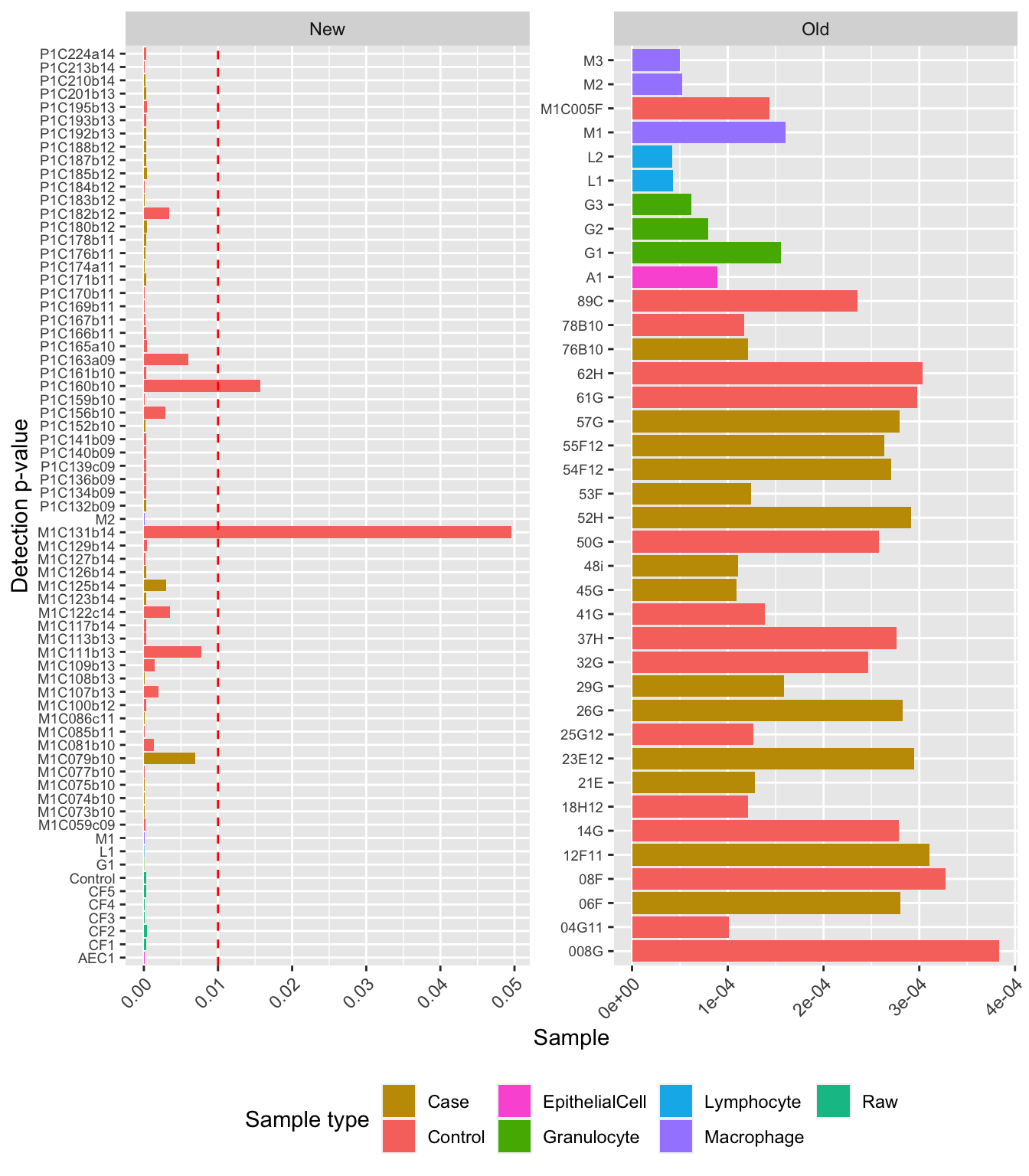
Sample filtering
Filter out samples with mean detection p-values > 0.01 to avoid filtering out too many probes downstream.
keep <- colMeans(detP) < 0.01
table(keep)
keep
FALSE TRUE
2 105 rgSet <- rgSet[, keep]
targets <- targets[keep, ]
detP <- detP[, keep]Normalisation
Normalise the data.
# normalize the data; this results in a GenomicRatioSet object
mSetSq <- preprocessQuantile(rgSet)
[preprocessQuantile] Mapping to genome.[preprocessQuantile] Fixing outliers.[preprocessQuantile] Quantile normalizing.mSetSqclass: GenomicRatioSet
dim: 865859 105
metadata(0):
assays(2): M CN
rownames(865859): cg14817997 cg26928153 ... cg07587934 cg16855331
rowData names(0):
colnames(105): 202900540100_R05C01 203013220097_R02C01 ...
204074230109_R07C01 204074230109_R08C01
colData names(15): Sample_ID Sample_Group ... yMed predictedSex
Annotation
array: IlluminaHumanMethylationEPIC
annotation: ilm10b4.hg19
Preprocessing
Method: Raw (no normalization or bg correction)
minfi version: 1.36.0
Manifest version: 0.3.0# create a MethylSet object from the raw data for plotting
mSetRaw <- preprocessRaw(rgSet)bSq <- getBeta(mSetSq)
bRaw <- getBeta(mSetRaw)
sq <- reshape2::melt(bSq)
sq$run <- targets$Sample_run
sq$type <- targets$Sample_Group
sq$process <- "Normalised"
raw <- reshape2::melt(bRaw)
raw$run <- targets$Sample_run
raw$type <- targets$Sample_Group
raw$process <- "Raw"
dat <- bind_rows(sq, raw)
colnames(dat)[1:3] <- c("cpg", "ID", "beta")
p1 <- ggplot(data = subset(dat, run == "Old"),
aes(x = beta, colour = type)) +
geom_density(show.legend = NA) +
labs(colour = "Sample type") +
facet_wrap(vars(process), ncol = 2) +
scale_color_manual(values = pal)
p2 <- ggplot(data = subset(dat, run == "New"),
aes(x = beta, colour = type)) +
geom_density() +
labs(colour = "Sample type") +
facet_wrap(vars(process), ncol = 2) +
scale_color_manual(values = pal)
(p1 / p2) +
plot_layout(guides = "collect") &
theme(legend.position = "bottom")Warning: Removed 655 rows containing non-finite values (stat_density).Warning: Removed 1147 rows containing non-finite values (stat_density).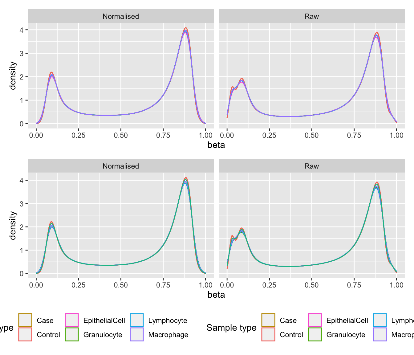
Data exploration (before filtering)
Explore the data to look for any structure. As expected, sex is the most significant source of variation. The patient samples, in particular, are clearly grouping by sex.
mDat <- getM(mSetSq)
mds <- plotMDS(mDat, top = 1000, gene.selection="common", plot = FALSE)
dat <- tibble(x = mds$x,
              y = mds$y,
              sample = targets$Sample_Group,
              run = targets$Sample_run,
              source = targets$Sample_source,
              sex = targets$Sex)

p1 <- ggplot(dat, aes(x = x, y = y, colour = sample)) +
  geom_point(aes(shape = run)) +
  labs(colour = "Sample type", shape = "Run",
       x = "Principal component 1",
       y = "Principal component 2") +
  ggtitle("All data") +
  scale_color_manual(values = pal)

p2 <- ggplot(dat, aes(x = x, y = y, colour = sex)) +
  geom_point(aes(shape = run)) +
  labs(colour = "Sample type", shape = "Run",
       x = "Principal component 1",
       y = "Principal component 2") +
  ggtitle("All data")

(p1 / p2) + plot_layout(guides = "collect")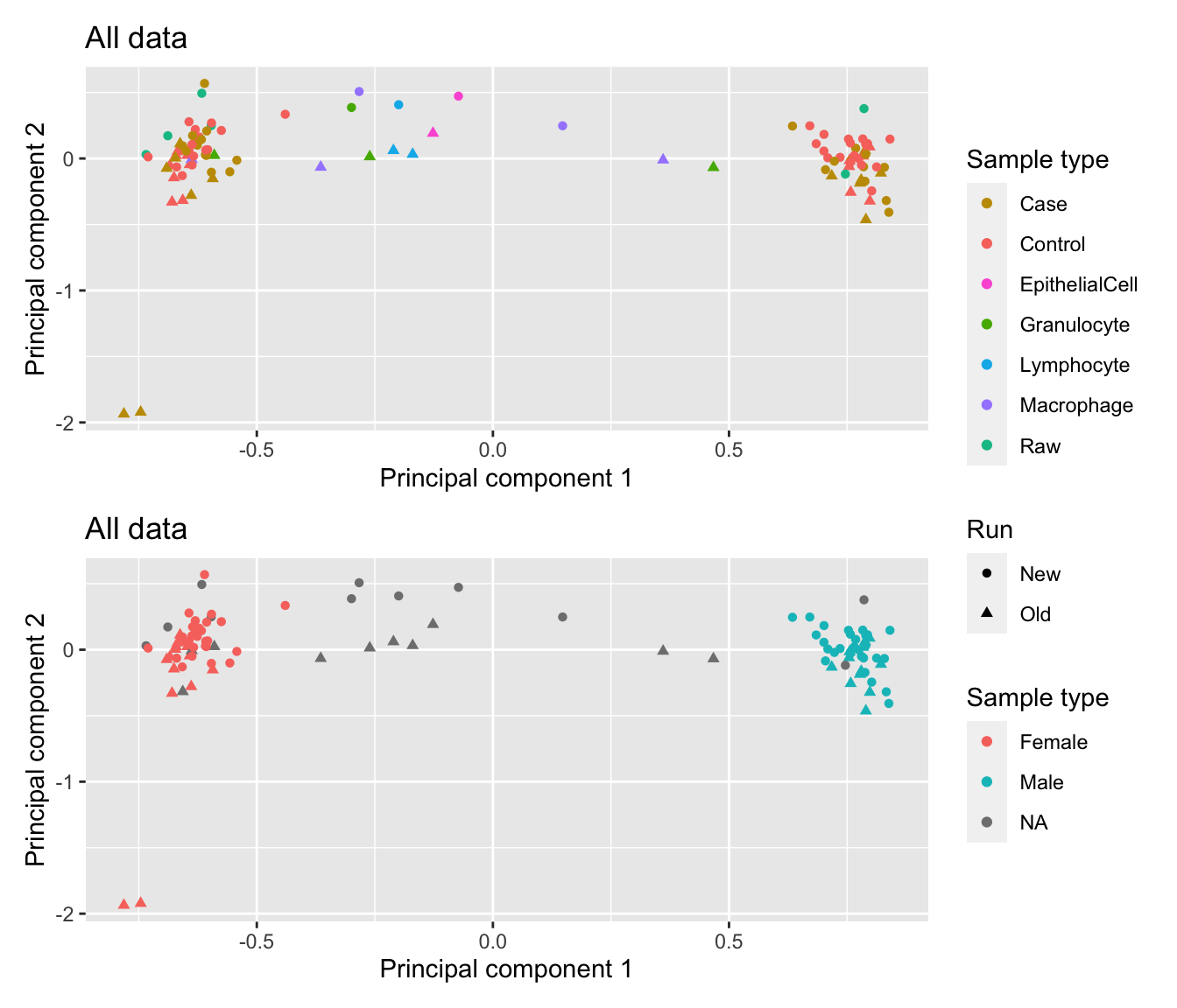
Colour ONLY the patient samples using different variables. Sex is driving all the variation in the first principal component of the patient samples, in both cohorts.
patients <- targets$Sample_Group %in% c("Case", "Control", "Raw")
mds <- plotMDS(mDat[, patients], top = 1000, gene.selection="common",
               plot = FALSE)
dat <- tibble(x = mds$x,
              y = mds$y,
              sample = targets$Sample_Group[patients],
              run = targets$Sample_run[patients],
              source = targets$Sample_source[patients],
              sex = targets$Sex[patients])

p1 <- ggplot(dat, aes(x = x, y = y, colour = sample)) +
  geom_point(aes(shape = run)) +
  labs(colour = "Sample type", shape = "Run",
       x = "Principal component 1",
       y = "Principal component 2") +
  ggtitle("Patients") +
  scale_color_manual(values = pal)

mds <- plotMDS(mDat[, targets$Sample_run %in% "Old" & patients], top = 1000,
               gene.selection="common", plot = FALSE)
dat <- tibble(x = mds$x,
              y = mds$y,
              sample = targets$Sample_Group[targets$Sample_run %in% "Old" &
                                              patients],
              run = targets$Sample_run[targets$Sample_run %in% "Old" &
                                         patients],
              source = targets$Sample_source[targets$Sample_run %in% "Old" & patients])

p2 <- ggplot(dat, aes(x = x, y = y, colour = sample)) +
  geom_point(show.legend = FALSE, shape = 1) +
  labs(colour = "Sample type",
       x = "Principal component 1",
       y = "Principal component 2") +
  ggtitle("Old run") +
  scale_color_manual(values = pal)

mds <- plotMDS(mDat[, targets$Sample_run %in% "New" & patients], top = 1000,
               gene.selection="common", plot = FALSE)
dat <- tibble(x = mds$x,
              y = mds$y,
              sample = targets$Sample_Group[targets$Sample_run %in% "New" &
                                              patients],
              run = targets$Sample_run[targets$Sample_run %in% "New" &
                                         patients],
              source = targets$Sample_source[targets$Sample_run %in% "New" &
                                       patients])

p3 <- ggplot(dat, aes(x = x, y = y, colour = sample)) +
  geom_point(show.legend = FALSE, shape = 1) +
  labs(colour = "Sample type",
       x = "Principal component 1",
       y = "Principal component 2") +
  ggtitle("New run") +
  scale_color_manual(values = pal)

mds <- plotMDS(mDat[, targets$Sample_run %in% "Old" & patients], top = 1000,
               gene.selection="common", plot = FALSE)
dat <- tibble(x = mds$x,
              y = mds$y,
              sample = targets$Sample_Group[targets$Sample_run %in% "Old" &
                                              patients],
              run = targets$Sample_run[targets$Sample_run %in% "Old" &
                                         patients],
              source = targets$Sample_source[targets$Sample_run %in% "Old" & patients],
              sex = targets$Sex[targets$Sample_run %in% "Old" & patients])

p4 <- ggplot(dat, aes(x = x, y = y, colour = sex)) +
  geom_point(shape = 1) +
  labs(colour = "Sex",
       x = "Principal component 1",
       y = "Principal component 2") +
  ggtitle("Old run")

mds <- plotMDS(mDat[, targets$Sample_run %in% "New" & patients], top = 1000,
               gene.selection="common", plot = FALSE)
dat <- tibble(x = mds$x,
              y = mds$y,
              sample = targets$Sample_Group[targets$Sample_run %in% "New" &
                                              patients],
              run = targets$Sample_run[targets$Sample_run %in% "New" &
                                         patients],
              source = targets$Sample_source[targets$Sample_run %in% "New" &
                                       patients],
              sex = targets$Sex[targets$Sample_run %in% "New" &
                                       patients])

p5 <- ggplot(dat, aes(x = x, y = y, colour = sex)) +
  geom_point(shape = 1) +
  labs(colour = "Sex",
       x = "Principal component 1",
       y = "Principal component 2") +
  ggtitle("New run")

p1 / (p2 | p3) / (p4 | p5) + plot_layout(guides = "collect")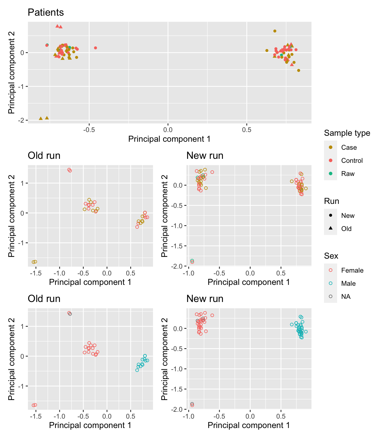
Colour ONLY the sorted cells samples using different variables. Encouragingly, the cell types cluster tightly when samples from both runs are combined, indicating that differences between cell types are more significant than any bath effects between the two runs. The cell types also cluster as expected for each of the individual runs.
cells <- !(targets$Sample_Group %in% c("Case", "Control", "Raw"))
mds <- plotMDS(mDat[, cells], top = 1000, gene.selection="common", plot = FALSE)
dat <- tibble(x = mds$x,
              y = mds$y,
              sample = targets$Sample_Group[cells],
              run = targets$Sample_run[cells],
              source = targets$Sample_source[cells])

p1 <- ggplot(dat, aes(x = x, y = y, colour = sample)) +
  geom_point(aes(shape = run)) +
  labs(colour = "Sample type", shape = "Run",
       x = "Principal component 1",
       y = "Principal component 2") +
  ggtitle("Cell types") +
  scale_color_manual(values = pal)

mds <- plotMDS(mDat[, targets$Sample_run %in% "Old" & cells], top = 1000,
               gene.selection="common", plot = FALSE)
dat <- tibble(x = mds$x,
              y = mds$y,
              sample = targets$Sample_Group[targets$Sample_run %in% "Old" &
                                              cells],
              run = targets$Sample_run[targets$Sample_run %in% "Old" &
                                         cells],
              source = targets$Sample_source[targets$Sample_run %in% "Old" & cells])

p2 <- ggplot(dat, aes(x = x, y = y, colour = sample)) +
  geom_point(show.legend = FALSE, shape = 1) +
  labs(colour = "Sample type",
       x = "Principal component 1",
       y = "Principal component 2") +
  ggtitle("Old run") +
  scale_color_manual(values = pal)

mds <- plotMDS(mDat[, targets$Sample_run %in% "New" & cells], top = 1000,
               gene.selection="common", plot = FALSE)
dat <- tibble(x = mds$x,
              y = mds$y,
              sample = targets$Sample_Group[targets$Sample_run %in% "New" &
                                              cells],
              run = targets$Sample_run[targets$Sample_run %in% "New" &
                                         cells],
              source = targets$Sample_source[targets$Sample_run %in% "New" &
                                       cells])

p3 <- ggplot(dat, aes(x = x, y = y, colour = sample)) +
  geom_point(show.legend = FALSE, shape = 1) +
  labs(colour = "Sample type",
       x = "Principal component 1",
       y = "Principal component 2") +
  ggtitle("New run") +
  scale_color_manual(values = pal)

p1 / (p2 | p3) + plot_layout(guides = "collect")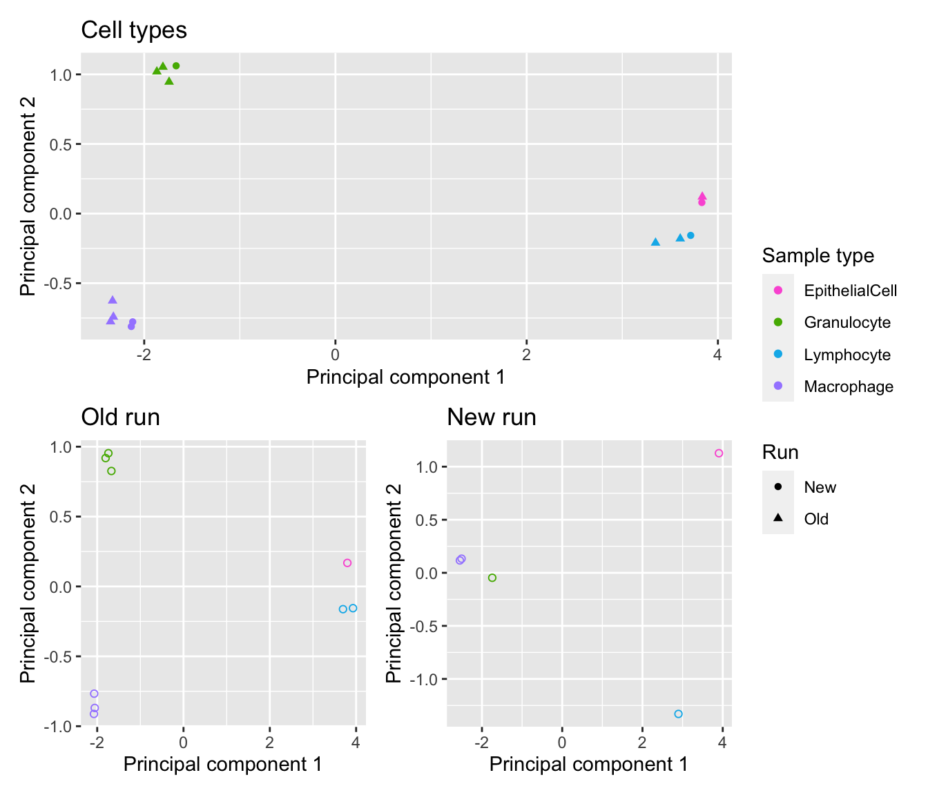
| Version | Author | Date |
|---|---|---|
| 2d78700 | JovMaksimovic | 2020-09-18 |
Filtering
Filter out poor performing probes, sex chromosome probes, SNP probes and cross reactive probes.
# ensure probes are in the same order in the mSetSq and detP objects
detP <- detP[match(featureNames(mSetSq), rownames(detP)),]
# remove any probes that have failed in one or more samples
keep <- rowSums(detP < 0.01) == ncol(mSetSq)
# subset data
mSetSqFlt <- mSetSq[keep,]
mSetSqFlt
class: GenomicRatioSet
dim: 818432 105
metadata(0):
assays(2): M CN
rownames(818432): cg14817997 cg26928153 ... cg07587934 cg16855331
rowData names(0):
colnames(105): 202900540100_R05C01 203013220097_R02C01 ...
204074230109_R07C01 204074230109_R08C01
colData names(15): Sample_ID Sample_Group ... yMed predictedSex
Annotation
array: IlluminaHumanMethylationEPIC
annotation: ilm10b4.hg19
Preprocessing
Method: Raw (no normalization or bg correction)
minfi version: 1.36.0
Manifest version: 0.3.0Calculate M and beta values for downstream use in analysis and visulalisation.
# calculate M-values and beta values for downstream analysis and visualisation
mVals <- getM(mSetSqFlt)
head(mVals[,1:5])
202900540100_R05C01 203013220097_R02C01 203013220097_R01C01
cg14817997 2.1578550 2.275865 2.5962535
cg26928153 2.2524546 2.237115 2.7532125
cg16269199 1.1801695 1.171997 1.6087922
cg13869341 2.7771918 2.678992 2.9783832
cg14008030 0.8272340 0.880665 0.6881874
cg12045430 -0.9479655 -1.082787 -0.8367633
202900540100_R06C01 202900540115_R01C01
cg14817997 1.5331122 1.6731574
cg26928153 2.7355681 2.2177367
cg16269199 1.6272844 1.2260346
cg13869341 2.7429478 2.3492332
cg14008030 0.4289779 0.8761655
cg12045430 -1.1153356 -0.9093120bVals <- getBeta(mSetSqFlt)
head(bVals[,1:5]) 202900540100_R05C01 203013220097_R02C01 203013220097_R01C01
cg14817997 0.8169339 0.8288515 0.8580985
cg26928153 0.8265373 0.8250076 0.8708372
cg16269199 0.6938182 0.6926135 0.7530842
cg13869341 0.8726953 0.8649394 0.8874004
cg14008030 0.6395462 0.6480390 0.6170428
cg12045430 0.3413959 0.3207056 0.3589326
202900540100_R06C01 202900540115_R01C01
cg14817997 0.7432009 0.7612863
cg26928153 0.8694553 0.8230599
cg16269199 0.7554599 0.7005299
cg13869341 0.8700348 0.8359455
cg14008030 0.5737933 0.6473273
cg12045430 0.3158107 0.3474454Remove SNP probes and multi-mapping probes.
mVals <- DMRcate::rmSNPandCH(mVals, mafcut = 0, rmcrosshyb = TRUE, rmXY = FALSE)
bVals <- DMRcate::rmSNPandCH(bVals, mafcut = 0, rmcrosshyb = TRUE, rmXY = FALSE)
dim(mVals)
[1] 711147 105Remove sex chromosome probes.
mValsNoXY <- DMRcate::rmSNPandCH(mVals, mafcut = 0, rmcrosshyb = TRUE,
                                 rmXY = TRUE)
bValsNoXY <- DMRcate::rmSNPandCH(bVals, mafcut = 0, rmcrosshyb = TRUE,
                                 rmXY = TRUE)
dim(mValsNoXY)
[1] 695764 105Data exploration (after filtering)
After filtering out poor performing probes, SNP probes and multi-mapping probes, the sex effect is much more pronounced in the first principal component of the data.
mds <- plotMDS(mVals, top = 1000, gene.selection="common", plot = FALSE)
dat <- tibble(x = mds$x,
              y = mds$y,
              sample = targets$Sample_Group,
              run = targets$Sample_run,
              source = targets$Sample_source,
              sex = targets$Sex)

p1 <- ggplot(dat, aes(x = x, y = y, colour = sample)) +
  geom_point(aes(shape = run)) +
  labs(colour = "Sample type", shape = "Run",
       x = "Principal component 1",
       y = "Principal component 2") +
  ggtitle("All data") +
  scale_color_manual(values = pal)

p2 <- ggplot(dat, aes(x = x, y = y, colour = sex)) +
  geom_point(aes(shape = run)) +
  labs(colour = "Sample type", shape = "Run",
       x = "Principal component 1",
       y = "Principal component 2") +
  ggtitle("All data")

(p1 / p2) + plot_layout(guides = "collect")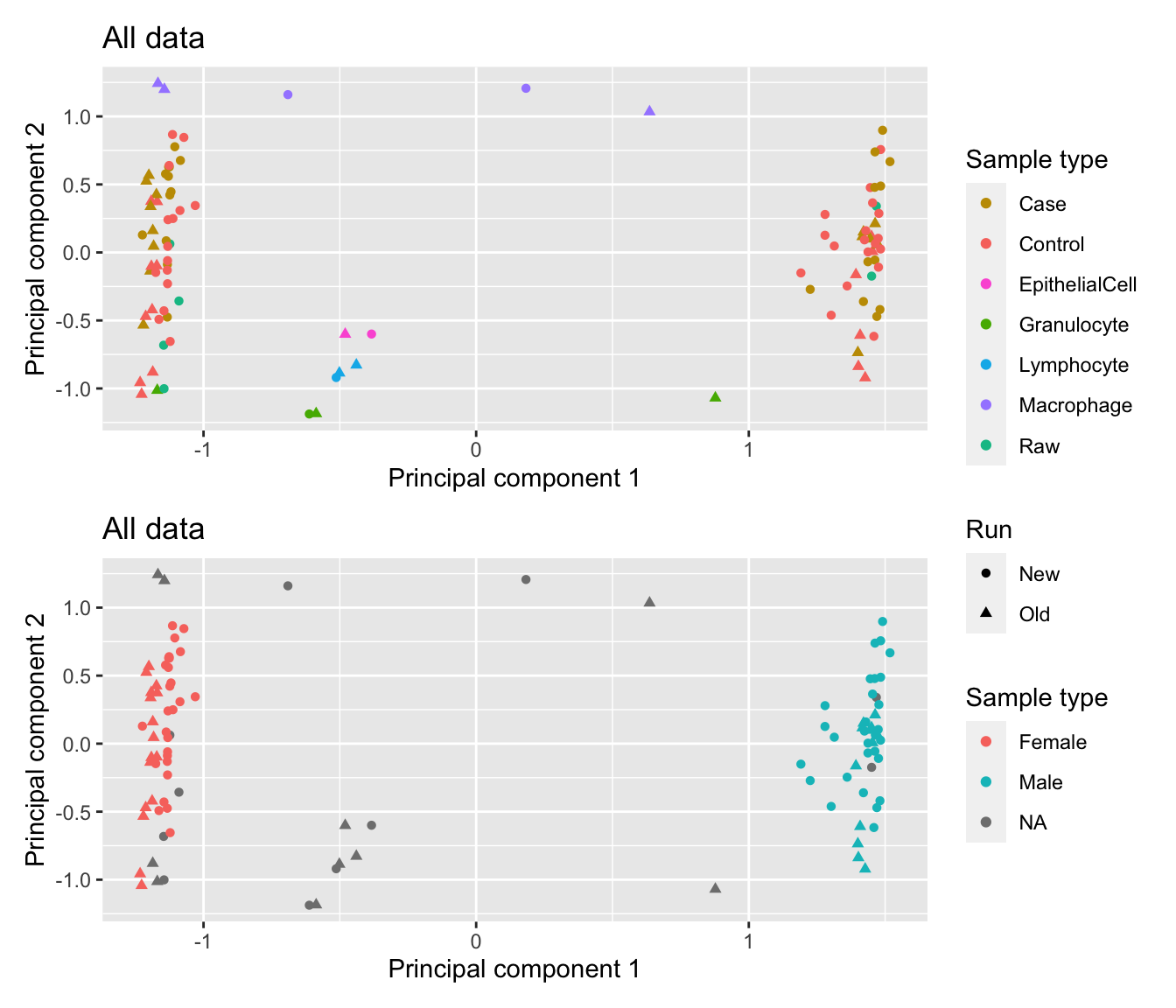
When the sex chromosome probes are also filtered out, the sex effect in the first principal component disappears. We now see that the difference between the sorted cells are driving the variation in the first two principal components. We also see some evidence of the batch effect between the two runs in the patients samples in the second principal component.
For the 9 year old cohort (old run), the control samples appear to be clustering towards the granulocyte samples suggesting that they may be dominated by that cell type. The first principal component appears to be capturing the differences between macrophages, granulocytes and lymphocytes whilst the second appears to be largely the difference between granulocytes and the other cell types. There is no evidence of skewing towards a particular cell type in the patient samples from the 1 year old cohort (new run).
mds <- plotMDS(mValsNoXY, top = 1000, gene.selection="common", plot = FALSE)
dat <- tibble(x = mds$x,
              y = mds$y,
              sample = targets$Sample_Group,
              run = targets$Sample_run,
              source = targets$Sample_source)

p1 <- ggplot(dat, aes(x = x, y = y, colour = sample)) +
  geom_point(aes(shape = run)) +
  labs(colour = "Sample type", shape = "Run",
       x = "Principal component 1",
       y = "Principal component 2") +
  ggtitle("All data") +
  scale_color_manual(values = pal)

mds <- plotMDS(mValsNoXY[, targets$Sample_run %in% "Old"], top = 1000,
               gene.selection="common", plot = FALSE)
dat <- tibble(x = mds$x,
              y = mds$y,
              sample = targets$Sample_Group[targets$Sample_run %in% "Old"],
              run = targets$Sample_run[targets$Sample_run %in% "Old"],
              source = targets$Sample_source[targets$Sample_run %in% "Old"])

p2 <- ggplot(dat, aes(x = x, y = y, colour = sample)) +
  geom_point(show.legend = FALSE, shape = 1) +
  labs(colour = "Sample type",
       x = "Principal component 1",
       y = "Principal component 2") +
  ggtitle("Old run") +
  scale_color_manual(values = pal) +
  geom_text(data = subset(dat, source %in% c("89C", "50G", "M1C005F", "04G11",
                                             "008G")),
            aes(label = source), size = 2, hjust = 0, colour = "black",
            nudge_x = 0.05)

mds <- plotMDS(mValsNoXY[, targets$Sample_run %in% "New"], top = 1000,
               gene.selection="common", plot = FALSE)
dat <- tibble(x = mds$x,
              y = mds$y,
              sample = targets$Sample_Group[targets$Sample_run %in% "New"],
              run = targets$Sample_run[targets$Sample_run %in% "New"],
              source = targets$Sample_source[targets$Sample_run %in% "New"])

p3 <- ggplot(dat, aes(x = x, y = y, colour = sample)) +
  geom_point(show.legend = FALSE, shape = 1) +
  labs(colour = "Sample type",
       x = "Principal component 1",
       y = "Principal component 2") +
  ggtitle("New run") +
  scale_color_manual(values = pal) +
  geom_text(data = subset(dat, source %in% c("DG", "IS")),
            aes(label = source), size = 2, hjust = 0, colour = "black",
            nudge_x = 0.05)

p1 / (p2 | p3) + plot_layout(guides = "collect")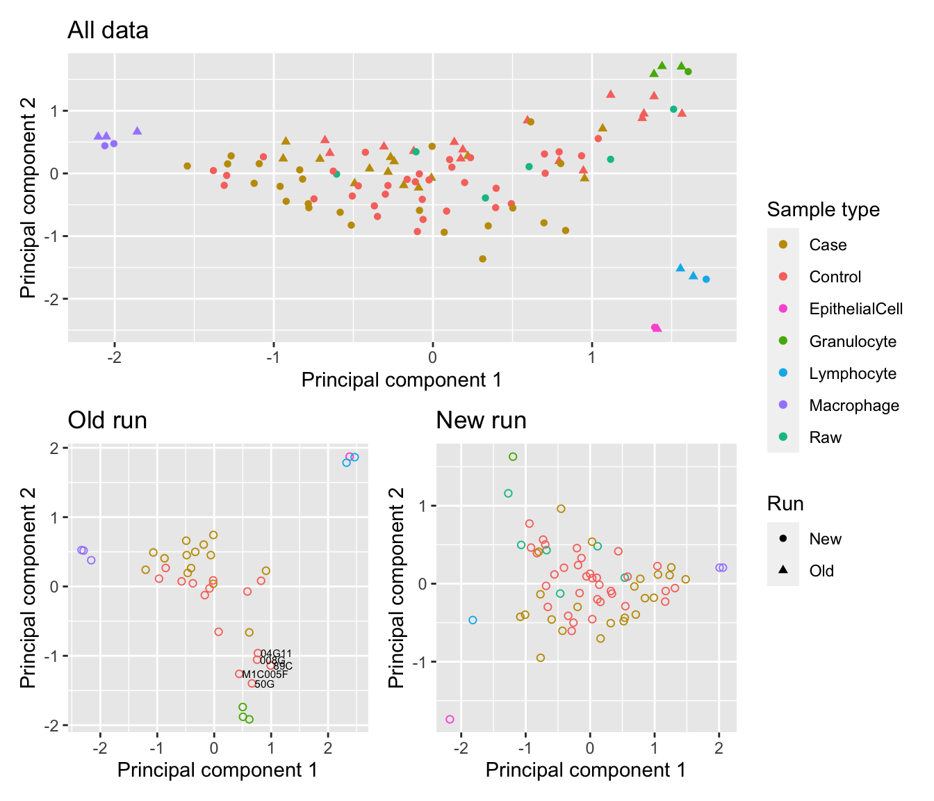
Looking at only the patient samples, the batch effect between the two runs is evident in the second principal component, although it is not severe. In the 9 year old cohort (old run), two samples (55F12 and 54F12) cluster away from the rest of the data in the second principal component. There is no obvious structure in the first two principal components for the 1 year old cohort (new run)
mds <- plotMDS(mValsNoXY[, patients], top = 1000, gene.selection="common", plot = FALSE)
dat <- tibble(x = mds$x,
              y = mds$y,
              sample = targets$Sample_Group[patients],
              run = targets$Sample_run[patients],
              source = targets$Sample_source[patients])

p1 <- ggplot(dat, aes(x = x, y = y, colour = sample)) +
  geom_point(aes(shape = run)) +
  labs(colour = "Sample type", shape = "Run",
       x = "Principal component 1",
       y = "Principal component 2") +
  ggtitle("Patients") +
  scale_color_manual(values = pal)

mds <- plotMDS(mValsNoXY[, targets$Sample_run %in% "Old" & patients], top = 1000,
               gene.selection="common", plot = FALSE)
dat <- tibble(x = mds$x,
              y = mds$y,
              sample = targets$Sample_Group[targets$Sample_run %in% "Old" &
                                              patients],
              run = targets$Sample_run[targets$Sample_run %in% "Old" &
                                         patients],
              source = targets$Sample_source[targets$Sample_run %in% "Old" & patients])

p2 <- ggplot(dat, aes(x = x, y = y, colour = sample)) +
  geom_point(show.legend = FALSE, shape = 1) +
  labs(colour = "Sample type",
       x = "Principal component 1",
       y = "Principal component 2") +
  ggtitle("Old run") +
  scale_color_manual(values = pal) +
  geom_text(data = subset(dat, source %in% c("55F12", "54F12")),
            aes(label = source), size = 2, hjust = 0, colour = "black",
            nudge_x = 0.05)

mds <- plotMDS(mValsNoXY[, targets$Sample_run %in% "New" & patients], top = 1000,
               gene.selection="common", plot = FALSE)
dat <- tibble(x = mds$x,
              y = mds$y,
              sample = targets$Sample_Group[targets$Sample_run %in% "New" &
                                              patients],
              run = targets$Sample_run[targets$Sample_run %in% "New" &
                                         patients],
              source = targets$Sample_source[targets$Sample_run %in% "New" &
                                       patients])

p3 <- ggplot(dat, aes(x = x, y = y, colour = sample)) +
  geom_point(show.legend = FALSE, shape = 1) +
  labs(colour = "Sample type",
       x = "Principal component 1",
       y = "Principal component 2") +
  ggtitle("New run") +
  scale_color_manual(values = pal)

p1 / (p2 | p3) + plot_layout(guides = "collect")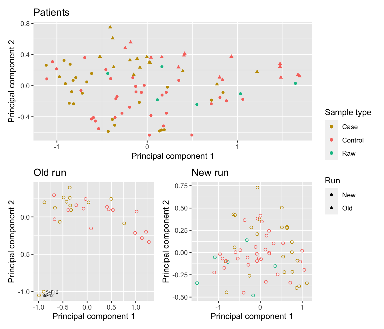
There is evidence of the batch effect between the two runs in the first two principal components. However, there is nothing obvious in the lower dimensions.
dims <- list(c(1,2), c(1,3), c(2,3), c(3,4))
p <- vector("list", length(dims))
for(i in 1:length(p)){
  mds <- plotMDS(mValsNoXY[, patients], top = 1000, gene.selection = "common",
                 plot = FALSE, dim.plot = dims[[i]])
  dat <- tibble(x = mds$x,
                y = mds$y,
                sample = targets$Sample_Group[patients],
                run = targets$Sample_run[patients],
                source = targets$Sample_source[patients])

  p[[i]] <- ggplot(dat, aes(x = x, y = y, colour = sample)) +
    geom_point(aes(shape = run)) +
    labs(colour = "Sample type", shape = "Run",
         x = glue("Principal component {dims[[i]][1]}"),
         y = glue("Principal component {dims[[i]][2]}")) +
    scale_color_manual(values = pal)

}

(p[[1]] | p[[2]]) / (p[[3]] | p[[4]]) + plot_layout(guides = "collect") +
  plot_annotation(title = "Patients")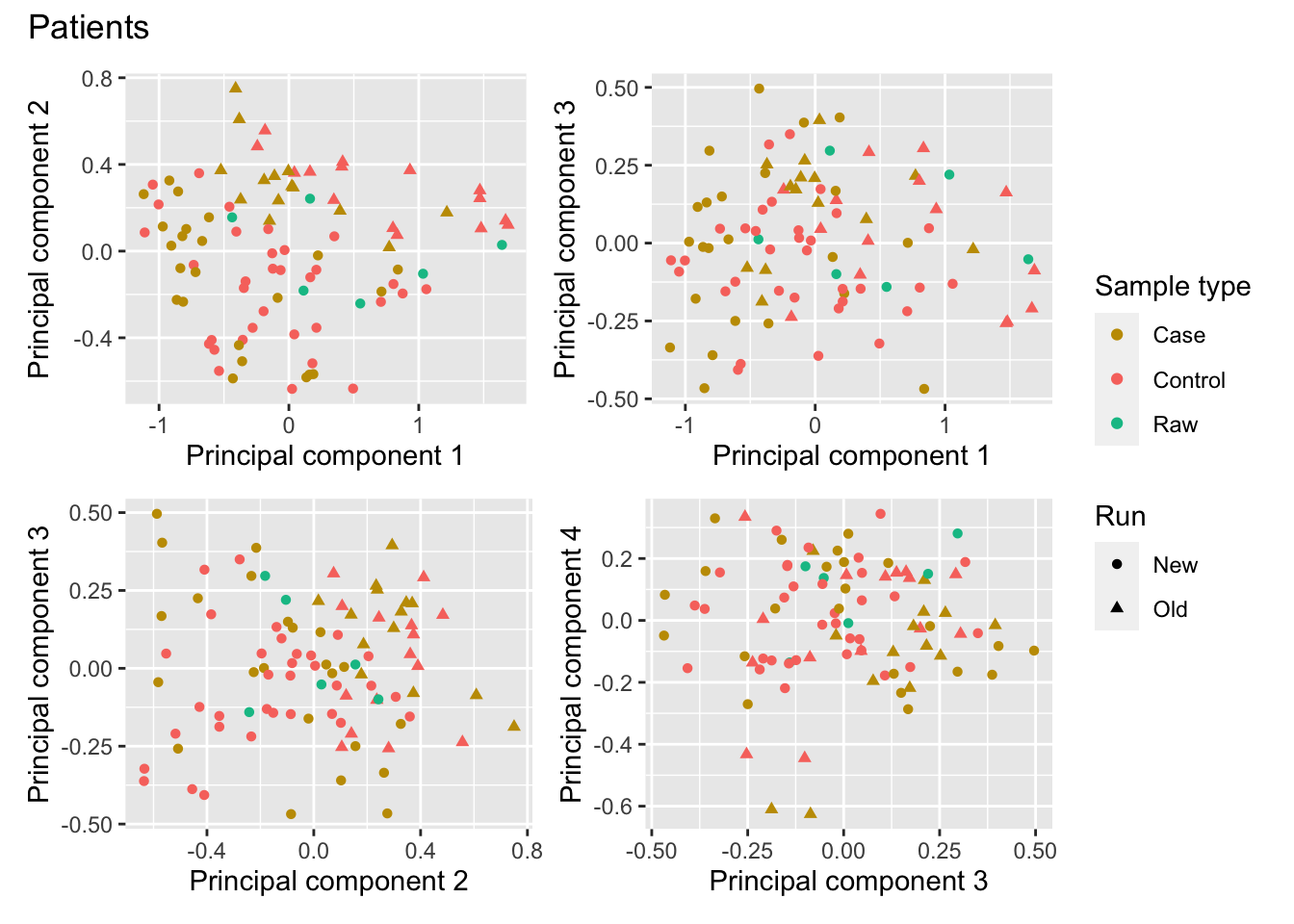
When we look at ONLY the sorted cell samples, the clustering by cell type is identical with or without the sex probes, indicating that sex is not a major srouce of variation in the sorted cell samples.
mds <- plotMDS(mVals[, cells], top = 1000, gene.selection="common", plot = FALSE)
dat <- tibble(x = mds$x,
              y = mds$y,
              sample = targets$Sample_Group[cells],
              run = targets$Sample_run[cells],
              source = targets$Sample_source[cells])

p1 <- ggplot(dat, aes(x = x, y = y, colour = sample)) +
  geom_point(aes(shape = run)) +
  labs(colour = "Sample type", shape = "Run",
       x = "Principal component 1",
       y = "Principal component 2") +
  ggtitle("Cell types: with sex probes") +
  scale_color_manual(values = pal)

mds <- plotMDS(mValsNoXY[, cells], top = 1000,
               gene.selection="common", plot = FALSE)
dat <- tibble(x = mds$x,
              y = mds$y,
              sample = targets$Sample_Group[cells],
              run = targets$Sample_run[cells],
              source = targets$Sample_source[cells])

p2 <- ggplot(dat, aes(x = x, y = y, colour = sample)) +
  geom_point(aes(shape = run)) +
  labs(colour = "Sample type",
       x = "Principal component 1",
       y = "Principal component 2") +
  ggtitle("Cell types: without sex probes") +
  scale_color_manual(values = pal)

(p1 / p2) + plot_layout(guides = "collect")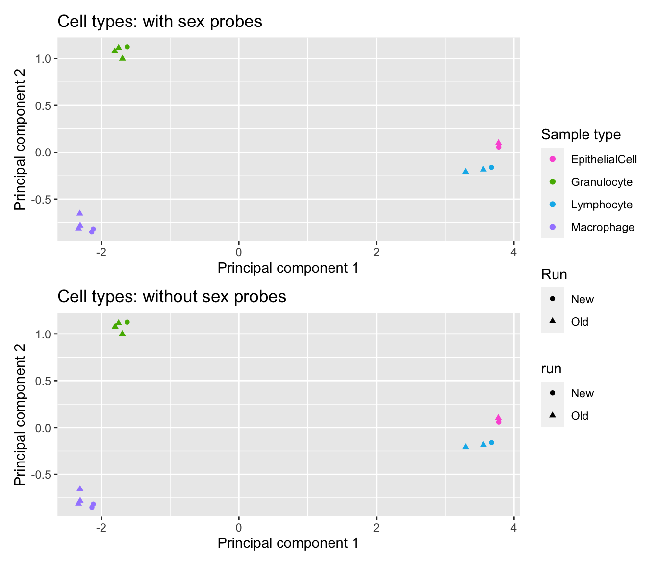
| Version | Author | Date |
|---|---|---|
| 2d78700 | JovMaksimovic | 2020-09-18 |
The batch effect between the two runs is also not a large source of variation in the sorted cell samples, as it is not evident in the first four principal components.
dims <- list(c(1,2), c(1,3), c(2,3), c(3,4))
p <- vector("list", length(dims))
for(i in 1:length(p)){
  mds <- plotMDS(mVals[, cells], top = 1000, gene.selection = "common",
                 plot = FALSE, dim.plot = dims[[i]])
  dat <- tibble(x = mds$x,
                y = mds$y,
                sample = targets$Sample_Group[cells],
                run = targets$Sample_run[cells],
                source = targets$Sample_source[cells])

  p[[i]] <- ggplot(dat, aes(x = x, y = y, colour = sample)) +
    geom_point(aes(shape = run)) +
    labs(colour = "Sample type", shape = "Run",
         x = glue("Principal component {dims[[i]][1]}"),
         y = glue("Principal component {dims[[i]][2]}")) +
    scale_color_manual(values = pal)

}

(p[[1]] | p[[2]]) / (p[[3]] | p[[4]]) + plot_layout(guides = "collect") +
  plot_annotation(title = "Cell types")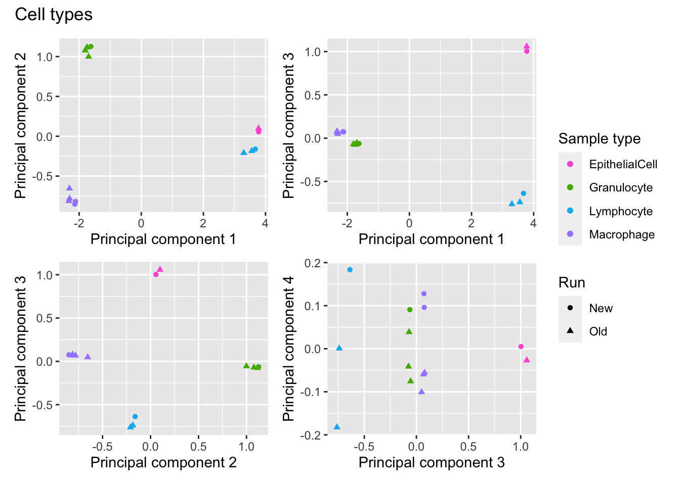
| Version | Author | Date |
|---|---|---|
| 2d78700 | JovMaksimovic | 2020-09-18 |
The data appears to be of good quality and shows no eivdence of unexpected sources of variation. Save the various data objects for faster downstream analysis.
outFile <- here("data/processedDataNew.RData")
if(!file.exists(outFile)){
  save(annEPIC, mSetSqFlt, rgSet, mVals, bVals, targets, mValsNoXY, bValsNoXY,
       pal, patients, cells, file = outFile)
}
sessionInfo()R version 4.0.3 (2020-10-10)
Platform: x86_64-apple-darwin17.0 (64-bit)
Running under: macOS Mojave 10.14.6
Matrix products: default
BLAS: /Library/Frameworks/R.framework/Versions/4.0/Resources/lib/libRblas.dylib
LAPACK: /Library/Frameworks/R.framework/Versions/4.0/Resources/lib/libRlapack.dylib
locale:
[1] en_AU.UTF-8/en_AU.UTF-8/en_AU.UTF-8/C/en_AU.UTF-8/en_AU.UTF-8
attached base packages:
[1] stats4 parallel stats graphics grDevices utils datasets
[8] methods base
other attached packages:
[1] DMRcatedata_2.8.0
[2] ExperimentHub_1.16.0
[3] AnnotationHub_2.22.0
[4] BiocFileCache_1.14.0
[5] dbplyr_2.0.0
[6] glue_1.4.2
[7] patchwork_1.1.1
[8] forcats_0.5.0
[9] dplyr_1.0.2
[10] purrr_0.3.4
[11] readr_1.4.0
[12] tidyr_1.1.2
[13] tibble_3.0.4
[14] ggplot2_3.3.2
[15] tidyverse_1.3.0
[16] IlluminaHumanMethylationEPICmanifest_0.3.0
[17] stringr_1.4.0
[18] minfiData_0.36.0
[19] IlluminaHumanMethylation450kmanifest_0.4.0
[20] missMethyl_1.24.0
[21] IlluminaHumanMethylationEPICanno.ilm10b4.hg19_0.6.0
[22] IlluminaHumanMethylation450kanno.ilmn12.hg19_0.6.0
[23] minfi_1.36.0
[24] bumphunter_1.32.0
[25] locfit_1.5-9.4
[26] iterators_1.0.13
[27] foreach_1.5.1
[28] Biostrings_2.58.0
[29] XVector_0.30.0
[30] SummarizedExperiment_1.20.0
[31] Biobase_2.50.0
[32] MatrixGenerics_1.2.0
[33] matrixStats_0.57.0
[34] GenomicRanges_1.42.0
[35] GenomeInfoDb_1.26.2
[36] IRanges_2.24.1
[37] S4Vectors_0.28.1
[38] BiocGenerics_0.36.0
[39] limma_3.46.0
[40] here_1.0.1
[41] workflowr_1.6.2
loaded via a namespace (and not attached):
[1] R.utils_2.10.1 tidyselect_1.1.0
[3] htmlwidgets_1.5.3 RSQLite_2.2.1
[5] AnnotationDbi_1.52.0 grid_4.0.3
[7] BiocParallel_1.24.1 munsell_0.5.0
[9] codetools_0.2-18 preprocessCore_1.52.0
[11] statmod_1.4.35 withr_2.3.0
[13] colorspace_2.0-0 knitr_1.30
[15] rstudioapi_0.13 labeling_0.4.2
[17] git2r_0.27.1 GenomeInfoDbData_1.2.4
[19] bit64_4.0.5 farver_2.0.3
[21] rhdf5_2.34.0 rprojroot_2.0.2
[23] vctrs_0.3.6 generics_0.1.0
[25] xfun_0.19 biovizBase_1.38.0
[27] R6_2.5.0 illuminaio_0.32.0
[29] AnnotationFilter_1.14.0 bitops_1.0-6
[31] rhdf5filters_1.2.0 reshape_0.8.8
[33] DelayedArray_0.16.0 assertthat_0.2.1
[35] bsseq_1.26.0 promises_1.1.1
[37] scales_1.1.1 nnet_7.3-14
[39] gtable_0.3.0 ensembldb_2.14.0
[41] rlang_0.4.9 genefilter_1.72.0
[43] splines_4.0.3 lazyeval_0.2.2
[45] rtracklayer_1.50.0 DSS_2.38.0
[47] GEOquery_2.58.0 dichromat_2.0-0
[49] checkmate_2.0.0 broom_0.7.3
[51] BiocManager_1.30.10 yaml_2.2.1
[53] reshape2_1.4.4 modelr_0.1.8
[55] GenomicFeatures_1.42.1 backports_1.2.1
[57] httpuv_1.5.4 Hmisc_4.4-2
[59] tools_4.0.3 nor1mix_1.3-0
[61] ellipsis_0.3.1 RColorBrewer_1.1-2
[63] siggenes_1.64.0 Rcpp_1.0.5
[65] plyr_1.8.6 base64enc_0.1-3
[67] sparseMatrixStats_1.2.0 progress_1.2.2
[69] zlibbioc_1.36.0 RCurl_1.98-1.2
[71] prettyunits_1.1.1 rpart_4.1-15
[73] openssl_1.4.3 haven_2.3.1
[75] cluster_2.1.0 fs_1.5.0
[77] magrittr_2.0.1 data.table_1.13.4
[79] reprex_0.3.0 whisker_0.4
[81] ProtGenerics_1.22.0 mime_0.9
[83] hms_0.5.3 evaluate_0.14
[85] xtable_1.8-4 XML_3.99-0.5
[87] jpeg_0.1-8.1 mclust_5.4.7
[89] readxl_1.3.1 gridExtra_2.3
[91] compiler_4.0.3 biomaRt_2.46.0
[93] crayon_1.3.4 R.oo_1.24.0
[95] htmltools_0.5.0 later_1.1.0.1
[97] Formula_1.2-4 lubridate_1.7.9.2
[99] DBI_1.1.0 MASS_7.3-53
[101] DMRcate_2.4.0 rappdirs_0.3.1
[103] Matrix_1.2-18 permute_0.9-5
[105] cli_2.2.0 R.methodsS3_1.8.1
[107] quadprog_1.5-8 Gviz_1.34.0
[109] pkgconfig_2.0.3 GenomicAlignments_1.26.0
[111] foreign_0.8-80 xml2_1.3.2
[113] annotate_1.68.0 rngtools_1.5
[115] multtest_2.46.0 beanplot_1.2
[117] rvest_0.3.6 doRNG_1.8.2
[119] scrime_1.3.5 VariantAnnotation_1.36.0
[121] digest_0.6.27 rmarkdown_2.6
[123] base64_2.0 cellranger_1.1.0
[125] htmlTable_2.1.0 edgeR_3.32.0
[127] DelayedMatrixStats_1.12.1 curl_4.3
[129] shiny_1.5.0 gtools_3.8.2
[131] Rsamtools_2.6.0 lifecycle_0.2.0
[133] nlme_3.1-151 jsonlite_1.7.2
[135] Rhdf5lib_1.12.0 askpass_1.1
[137] BSgenome_1.58.0 fansi_0.4.1
[139] pillar_1.4.7 lattice_0.20-41
[141] fastmap_1.0.1 httr_1.4.2
[143] survival_3.2-7 interactiveDisplayBase_1.28.0
[145] png_0.1-7 BiocVersion_3.12.0
[147] bit_4.0.4 stringi_1.5.3
[149] HDF5Array_1.18.0 blob_1.2.1
[151] org.Hs.eg.db_3.12.0 latticeExtra_0.6-29
[153] memoise_1.1.0