Estimating cell proportions
Jovana Maksimovic
12/17/2018
Last updated: 2020-12-18
Checks: 7 0
Knit directory: paed-cf-methylation/
This reproducible R Markdown analysis was created with workflowr (version 1.6.2). The Checks tab describes the reproducibility checks that were applied when the results were created. The Past versions tab lists the development history.
Great! Since the R Markdown file has been committed to the Git repository, you know the exact version of the code that produced these results.
Great job! The global environment was empty. Objects defined in the global environment can affect the analysis in your R Markdown file in unknown ways. For reproduciblity it's best to always run the code in an empty environment.
The command set.seed(20200224) was run prior to running the code in the R Markdown file. Setting a seed ensures that any results that rely on randomness, e.g. subsampling or permutations, are reproducible.
Great job! Recording the operating system, R version, and package versions is critical for reproducibility.
Nice! There were no cached chunks for this analysis, so you can be confident that you successfully produced the results during this run.
Great job! Using relative paths to the files within your workflowr project makes it easier to run your code on other machines.
Great! You are using Git for version control. Tracking code development and connecting the code version to the results is critical for reproducibility.
The results in this page were generated with repository version 667bbf7. See the Past versions tab to see a history of the changes made to the R Markdown and HTML files.
Note that you need to be careful to ensure that all relevant files for the analysis have been committed to Git prior to generating the results (you can use wflow_publish or wflow_git_commit). workflowr only checks the R Markdown file, but you know if there are other scripts or data files that it depends on. Below is the status of the Git repository when the results were generated:
Ignored files:
    Ignored:    .DS_Store
    Ignored:    .Rhistory
    Ignored:    .Rproj.user/
    Ignored:    code/DNAm-based-age-predictor/
    Ignored:    data/.DS_Store
    Ignored:    data/1-year-old-cohort-with-data.csv
    Ignored:    data/9-year-old-cohort-as-pairs-with-data.csv
    Ignored:    data/9-year-old-cohort-as-pairs.xlsx
    Ignored:    data/BMI-Data.csv
    Ignored:    data/BMI-Data.xlsx
    Ignored:    data/CFGeneModifiers.csv
    Ignored:    data/Flow-Data-for-Reference-Panel-Original copy.csv
    Ignored:    data/Flow-Data-for-Reference-Panel-Original.csv
    Ignored:    data/Flow-Data-for-Reference-Panel-Scaled copy.csv
    Ignored:    data/Flow-Data-for-Reference-Panel-Scaled.csv
    Ignored:    data/Flow-Data-for-Reference-Panel.xls
    Ignored:    data/Horvath-27k-probes.csv
    Ignored:    data/Horvath-coefficients.csv
    Ignored:    data/Horvath-methylation-data.csv
    Ignored:    data/Horvath-mini-annotation.csv
    Ignored:    data/Horvath-sample-data.csv
    Ignored:    data/ageFile-final.txt
    Ignored:    data/arsq.rds
    Ignored:    data/idat-new/
    Ignored:    data/idat/
    Ignored:    data/loglrt.rds
    Ignored:    data/processedData.RData
    Ignored:    data/processedDataNew-old.RData
    Ignored:    data/processedDataNew.RData
    Ignored:    data/rawPatientBetas.rds
    Ignored:    data/~$9-year-old-cohort-as-pairs.xlsx
    Ignored:    output/Horvath-output.csv
    Ignored:    output/Horvath-output2.csv
    Ignored:    output/age.pred
    Ignored:    output/case-ctrl-oneyr-ruv-sig-adj-betas-expanded.csv
    Ignored:    output/case-ctrl-oneyr-ruv-sig-adj-betas.csv
    Ignored:    output/case-ctrl-oneyr-ruv.csv
    Ignored:    output/case-ctrl-oneyr.csv
    Ignored:    output/case-ctrl-paired.csv
    Ignored:    output/stderr.txt
    Ignored:    output/stdout.txt

Untracked files:
    Untracked:  MethylResolver.txt
    Untracked:  code/test.R
Note that any generated files, e.g. HTML, png, CSS, etc., are not included in this status report because it is ok for generated content to have uncommitted changes.
These are the previous versions of the repository in which changes were made to the R Markdown (analysis/estCellPropNew.Rmd) and HTML (docs/estCellPropNew.html) files. If you've configured a remote Git repository (see ?wflow_git_remote), click on the hyperlinks in the table below to view the files as they were in that past version.
| File | Version | Author | Date | Message |
|---|---|---|---|---|
| Rmd | 667bbf7 | JovMaksimovic | 2020-12-18 | wflow_publish(c("analysis/estCellPropNew.Rmd")) |
| html | 83b3f2e | JovMaksimovic | 2020-12-18 | Build site. |
| Rmd | a54eaf6 | JovMaksimovic | 2020-12-18 | wflow_publish(c("analysis/dataExploreNew.Rmd", "analysis/estCellPropNew.Rmd", |
| html | ac6a20c | JovMaksimovic | 2020-10-30 | Build site. |
| Rmd | 7783fb1 | JovMaksimovic | 2020-10-30 | analysis/oneYearAnalysis.Rmd |
| html | 2d78700 | JovMaksimovic | 2020-09-18 | Build site. |
| Rmd | 4eae19b | JovMaksimovic | 2020-09-18 | wflow_publish(c("analysis/index.Rmd", "analysis/dataExploreNew.Rmd", |
| html | f656443 | JovMaksimovic | 2020-08-31 | Build site. |
| Rmd | e449b94 | JovMaksimovic | 2020-08-31 | wflow_publish(c("analysis/index.Rmd", "analysis/estCellPropNew.Rmd")) |
| html | 1add90b | JovMaksimovic | 2020-07-31 | Build site. |
| Rmd | d3f4072 | JovMaksimovic | 2020-07-31 | wflow_publish(c("analysis/index.Rmd", "analysis/dataExploreNew.Rmd", |
| Rmd | 32544d7 | JovMaksimovic | 2020-07-28 | Analysis including new variables and cell proportion estimation using both datasets. |
Estimate cell type proportions of BAL patient samples
Load all necessary analysis packages.
library(here)
library(workflowr)
library(glue)
#Load Packages Required for Analysis
library(limma)
library(minfi)
library(matrixStats)
library(IlluminaHumanMethylationEPICanno.ilm10b4.hg19)
library(IlluminaHumanMethylationEPICmanifest)
library(FlowSorted.Blood.EPIC)
library(ggplot2)
library(ExperimentHub)
library(reshape2)
library(tidyverse)
library(patchwork)
Load raw and processed data objects generated by exploratory analysis.
# load data objects
load(here("data/processedDataNew.RData"))
# load modified cell type estimation function
source(here("code/functions.R"))
As expected, we see clear clustering by cell types.
mds <- plotMDS(mVals[, cells], top = 1000, gene.selection="common", plot = FALSE)
dat <- tibble(x = mds$x,
              y = mds$y,
              sample = targets$Sample_Group[cells],
              run = targets$Sample_run[cells],
              ID = targets$Sample_ID[cells])

p <- ggplot(dat, aes(x = x, y = y, colour = sample)) +
  geom_point(aes(shape = run)) +
  labs(colour = "Sample type", shape = "Run",
       x = "Principal component 1",
       y = "Principal component 2") +
  ggtitle("Cell types") +
  scale_color_manual(values = pal)
p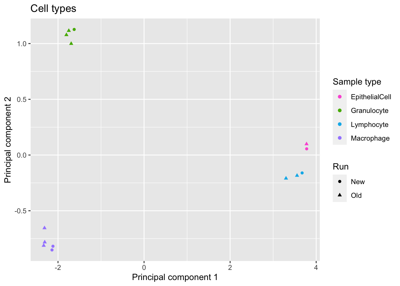
Reference panel validation
We will use blood immune cell mixtures with known cell type proportions published by Salas et al. 2018 to test the accuracy of cell type proportion estimates derived using our reference library.
hub <- ExperimentHub() snapshotDate(): 2020-10-02query(hub, "FlowSorted.Blood.EPIC") ExperimentHub with 1 record
# snapshotDate(): 2020-10-02
# names(): EH1136
# package(): FlowSorted.Blood.EPIC
# $dataprovider: GEO
# $species: Homo sapiens
# $rdataclass: RGChannelSet
# $rdatadateadded: 2018-04-20
# $title: FlowSorted.Blood.EPIC: Illumina Human Methylation data from EPIC o...
# $description: The FlowSorted.Blood.EPIC package contains Illumina HumanMet...
# $taxonomyid: 9606
# $genome: hg19
# $sourcetype: tar.gz
# $sourceurl: https://www.ncbi.nlm.nih.gov/geo/query/acc.cgi?acc=GSE110554
# $sourcesize: NA
# $tags: c("ExperimentData", "Homo_sapiens_Data", "Tissue",
# "MicroarrayData", "Genome", "TissueMicroarrayData",
# "MethylationArrayData")
# retrieve record with 'object[["EH1136"]]' FlowSorted.Blood.EPIC <- hub[["EH1136"]]see ?FlowSorted.Blood.EPIC and browseVignettes('FlowSorted.Blood.EPIC') for documentationloading from cache# separate the reference from the testing dataset
RGsetTargets <- FlowSorted.Blood.EPIC[,FlowSorted.Blood.EPIC$CellType == "MIX"]
mixReal <- as.matrix(colData(RGsetTargets)[,12:17])/100mixDat <- melt(mixReal)
colnames(mixDat) <- c("sample","cell","proportion")
p <- ggplot(mixDat, aes(sample)) +
geom_bar(aes(fill = cell, weight=proportion)) +
scale_x_discrete(breaks = waiver(), labels=1:nrow(mixReal)) +
ggtitle("Artificially created cell mixtures") +
labs(y = "Proportion", x = "Mixture", fill = "Cell type")
p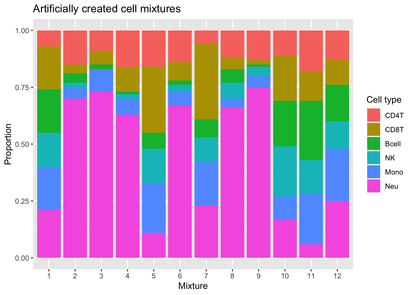
| Version | Author | Date |
|---|---|---|
| 1add90b | JovMaksimovic | 2020-07-31 |
We have not sorted our BAL lymphocytes into B cells, T cells and NK cells, so the "true" lymphocyte value we will compare to is the sum of the proportions of those cells in the artificial mixture.
mixSum <- data.frame(mixReal[,5:6], Lymph = rowSums(mixReal[,1:4]))
mixSumDat <- melt(as.matrix(mixSum))
colnames(mixSumDat) <- c("sample","cell","proportion")

p <- ggplot(mixSumDat, aes(sample)) +
  geom_bar(aes(fill = cell, weight = proportion)) +
    scale_x_discrete(breaks = waiver(), labels = 1:nrow(mixReal)) +
    ggtitle("Artificially created cell mixtures") +
  labs(y = "Proportion", x = "Mixture", fill = "Cell type")
p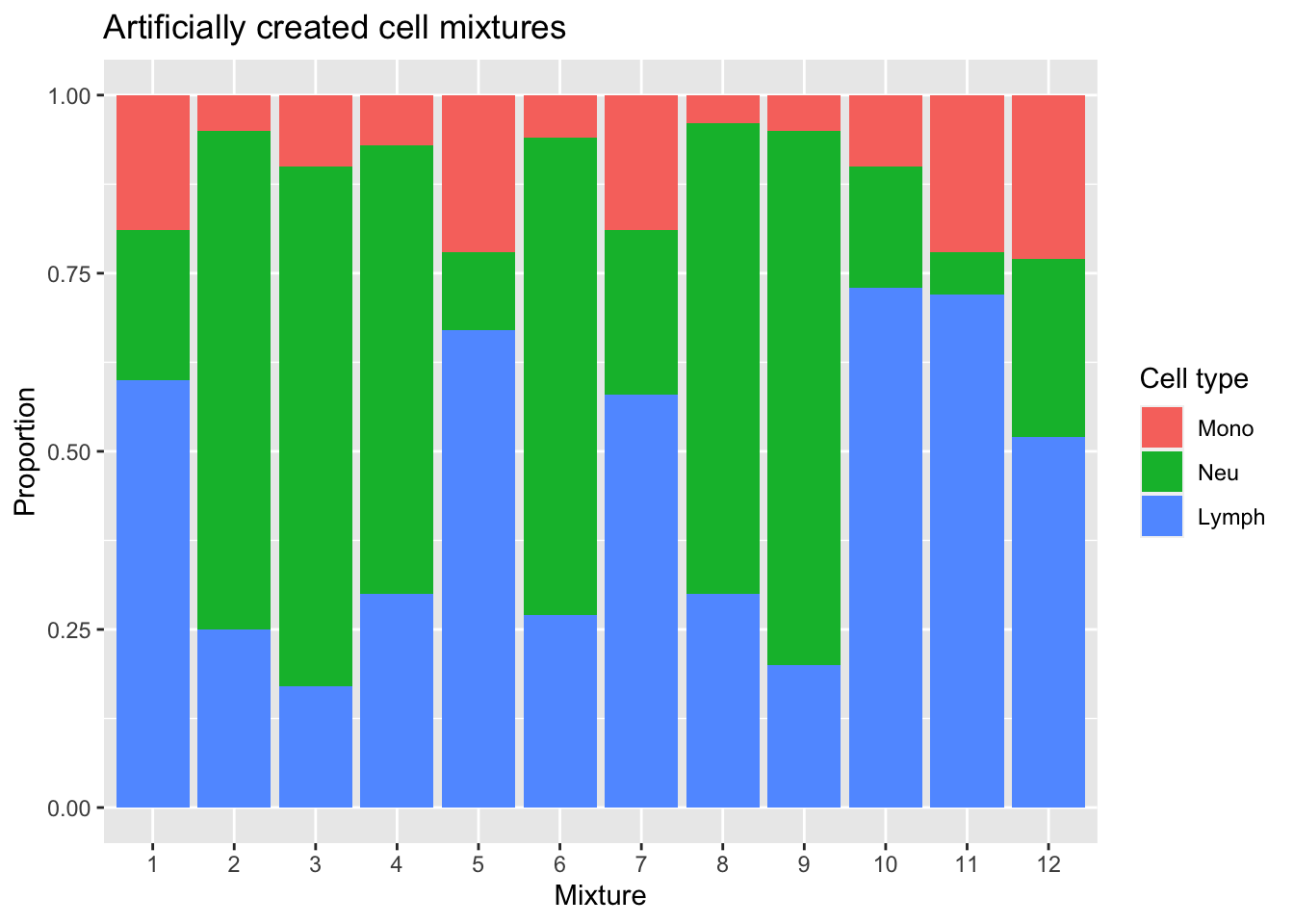
| Version | Author | Date |
|---|---|---|
| 1add90b | JovMaksimovic | 2020-07-31 |
Estimate cell type proportions in artificial mixture using both option.
lavageRef <- rgSet[,cells]
colData(lavageRef)$CellType <- colData(lavageRef)$Sample_Group
mixEstBoth <- estimateCellCounts2Mod(rgSet = RGsetTargets,
                                  compositeCellType = "Lavage",
                                  processMethod = "preprocessQuantile",
                                  probeSelect = "both",
                                  cellTypes = unique(targets$Sample_Group[cells]),
                                  referencePlatform =
                                    "IlluminaHumanMethylationEPIC",
                                  referenceset = "lavageRef",
                                  IDOLOptimizedCpGs = NULL,
                                  returnAll = FALSE,
                                  meanPlot = FALSE,
                                  keepProbes = rownames(mValsNoXY))
[estimateCellCounts2] Combining user data with reference (flow sorted) data.Warning in DataFrame(sampleNames = c(colnames(rgSet),
colnames(referenceRGset)), : 'stringsAsFactors' is ignored[estimateCellCounts2] Processing user and reference data together.[preprocessQuantile] Mapping to genome.Warning in .getSex(CN = CN, xIndex = xIndex, yIndex = yIndex, cutoff = cutoff):
An inconsistency was encountered while determining sex. One possibility is
that only one sex is present. We recommend further checks, for example with the
plotSex function.[preprocessQuantile] Fixing outliers.[preprocessQuantile] Quantile normalizing.[estimateCellCounts2] Picking probes for composition estimation.[estimateCellCounts2] Estimating composition.mixEstBoth$counts EpithelialCell Macrophage Granulocyte Lymphocyte
201868590193_R01C01 0.000000e+00 9.556121e-02 0.3604522 0.5629822
201868590243_R02C01 0.000000e+00 -9.601278e-19 0.7382592 0.2615245
201868590267_R01C01 0.000000e+00 2.010882e-02 0.7773913 0.2022645
201868590267_R05C01 -1.235089e-18 0.000000e+00 0.6786281 0.3195772
201869680008_R01C01 0.000000e+00 9.224650e-02 0.2578286 0.6626807
201869680008_R03C01 -1.567380e-18 0.000000e+00 0.7125502 0.2825512
201869680008_R06C01 -4.336809e-19 7.890393e-02 0.3646301 0.5630572
201869680030_R03C01 0.000000e+00 -1.050283e-18 0.7012296 0.3043583
201869680030_R07C01 1.734723e-18 -1.316556e-18 0.7752668 0.2218530
201870610056_R01C01 0.000000e+00 3.767229e-02 0.2969845 0.6825515
201870610056_R03C01 0.000000e+00 1.159349e-01 0.2223959 0.6817935
201870610111_R03C01 0.000000e+00 1.053280e-01 0.4028818 0.5024397mixBoth <- reshape2::melt(mixEstBoth$counts)
colnames(mixBoth) <- c("sample","cell","proportion")
p1 <- ggplot(mixBoth, aes(x = sample, fill = cell)) +
geom_bar(aes(weight = proportion)) +
ggtitle("Cell type proportion estimates",
subtitle = "Probe selection: Both") +
labs(x = "Sample", y = "Proportion", fill = "Cell type") +
scale_x_discrete(breaks = waiver(), labels = 1:nrow(mixReal)) +
scale_fill_manual(values = pal)
p1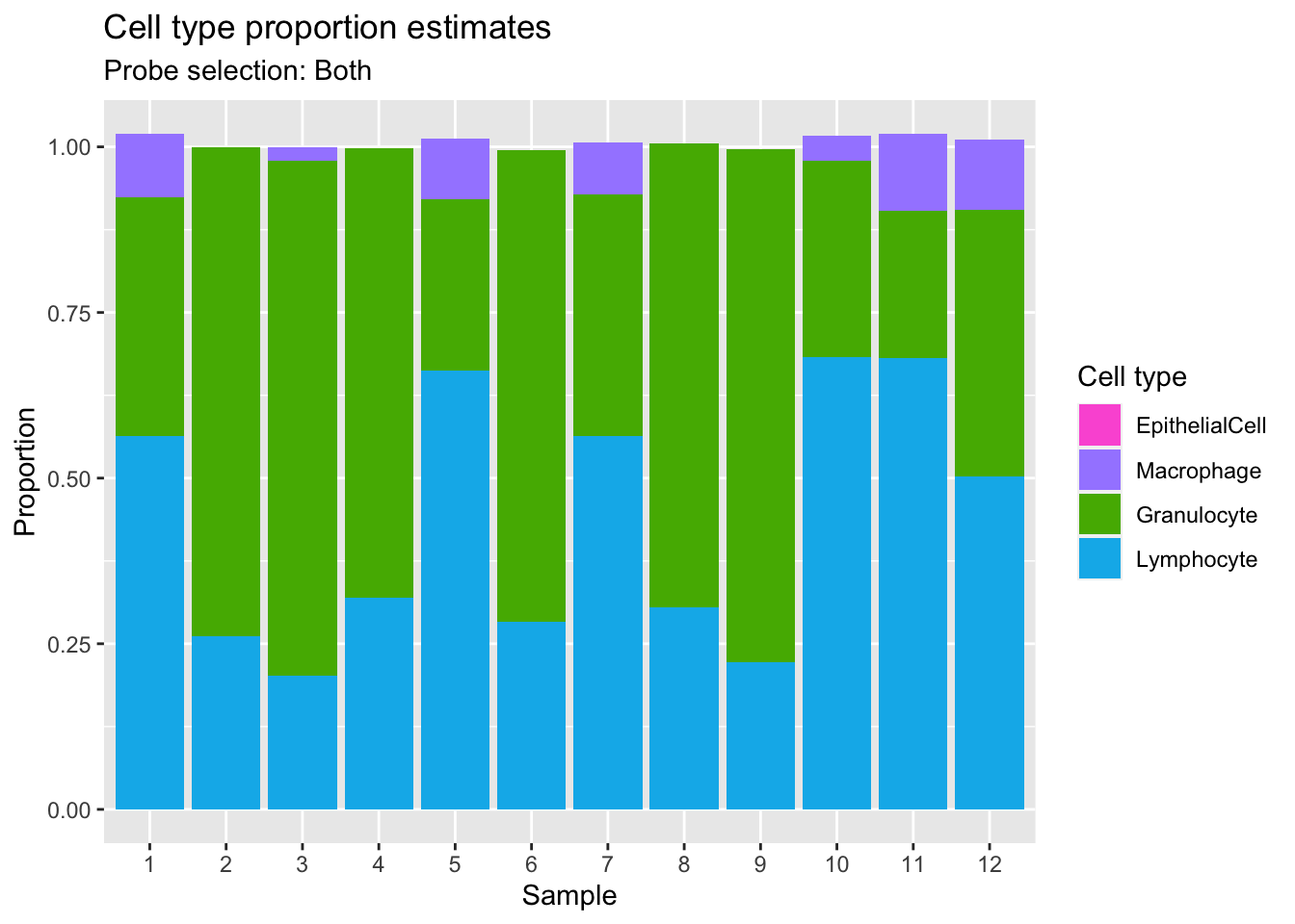
| Version | Author | Date |
|---|---|---|
| 1add90b | JovMaksimovic | 2020-07-31 |
(p | p1) +
  plot_layout(guides = "collect") &
  theme(legend.position = "bottom",
        legend.box = "vertical")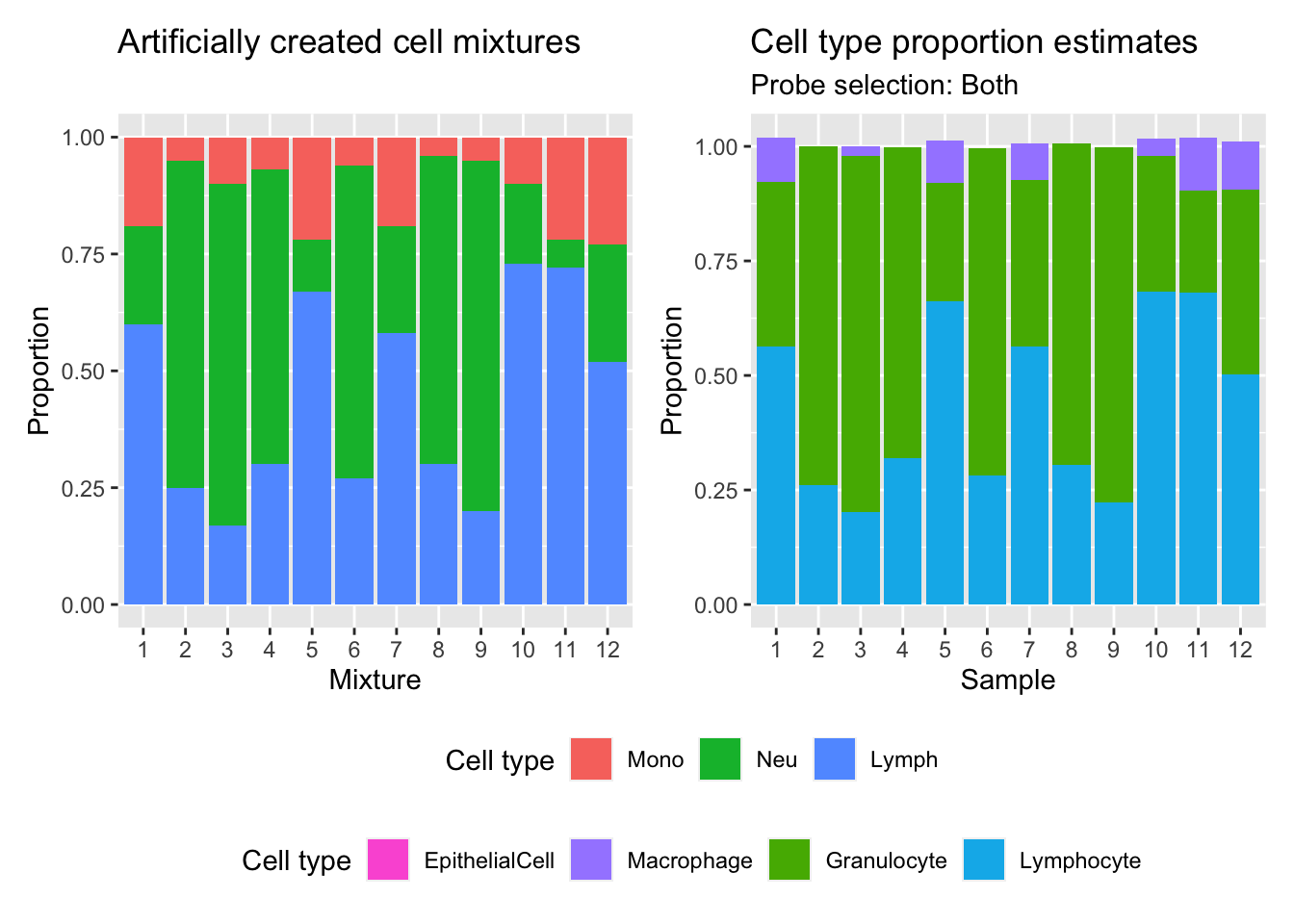
| Version | Author | Date |
|---|---|---|
| 1add90b | JovMaksimovic | 2020-07-31 |
Estimate cell type proportions in artificial mixture using any option.
mixEstAny <- estimateCellCounts2Mod(rgSet = RGsetTargets,
                                 compositeCellType = "Lavage",
                                processMethod = "preprocessQuantile",
                                probeSelect = "any",
                                cellTypes = unique(targets$Sample_Group[cells]),
                                referencePlatform =
                                "IlluminaHumanMethylationEPIC",
                                referenceset = "lavageRef",
                                IDOLOptimizedCpGs = NULL,
                                returnAll = FALSE,
                                meanPlot = FALSE,
                                keepProbes = rownames(mValsNoXY))
[estimateCellCounts2] Combining user data with reference (flow sorted) data.Warning in DataFrame(sampleNames = c(colnames(rgSet),
colnames(referenceRGset)), : 'stringsAsFactors' is ignored[estimateCellCounts2] Processing user and reference data together.[preprocessQuantile] Mapping to genome.Warning in .getSex(CN = CN, xIndex = xIndex, yIndex = yIndex, cutoff = cutoff):
An inconsistency was encountered while determining sex. One possibility is
that only one sex is present. We recommend further checks, for example with the
plotSex function.[preprocessQuantile] Fixing outliers.[preprocessQuantile] Quantile normalizing.[estimateCellCounts2] Picking probes for composition estimation.[estimateCellCounts2] Estimating composition.mixEstAny$counts EpithelialCell Macrophage Granulocyte Lymphocyte
201868590193_R01C01 0.000000e+00 0.152280346 0.3031935 0.5711907
201868590243_R02C01 0.000000e+00 0.008172784 0.7257607 0.2653215
201868590267_R01C01 -1.734723e-18 0.048245288 0.7566930 0.2020889
201868590267_R05C01 0.000000e+00 0.021316730 0.6632601 0.3185858
201869680008_R01C01 0.000000e+00 0.162484376 0.2138915 0.6569458
201869680008_R03C01 0.000000e+00 0.012936076 0.7032285 0.2817858
201869680008_R06C01 0.000000e+00 0.133760469 0.3275543 0.5593185
201869680030_R03C01 0.000000e+00 0.005767843 0.6800623 0.3136724
201869680030_R07C01 0.000000e+00 0.003937728 0.7685961 0.2241918
201870610056_R01C01 0.000000e+00 0.081121286 0.2386478 0.6940527
201870610056_R03C01 0.000000e+00 0.185915449 0.1498483 0.6921916
201870610111_R03C01 0.000000e+00 0.168102490 0.3513066 0.5037587mixAny <- reshape2::melt(mixEstAny$counts)
colnames(mixAny) <- c("sample","cell","proportion")
p2 <- ggplot(mixAny, aes(x = sample, fill = cell)) +
geom_bar(aes(weight = proportion)) +
ggtitle("Cell type proportion estimates",
subtitle = "Probe selection: Any") +
labs(x = "Sample", y = "Proportion", fill = "Cell type") +
scale_x_discrete(breaks = waiver(), labels = 1:nrow(mixReal)) +
scale_fill_manual(values = pal)
p2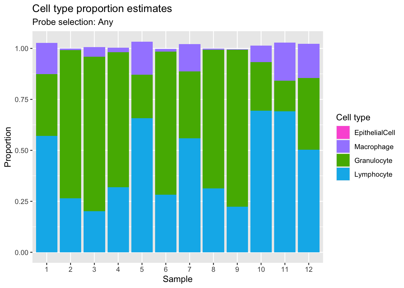
| Version | Author | Date |
|---|---|---|
| 1add90b | JovMaksimovic | 2020-07-31 |
(p | p2) +
  plot_layout(guides = "collect") &
  theme(legend.position = "bottom",
        legend.box = "vertical")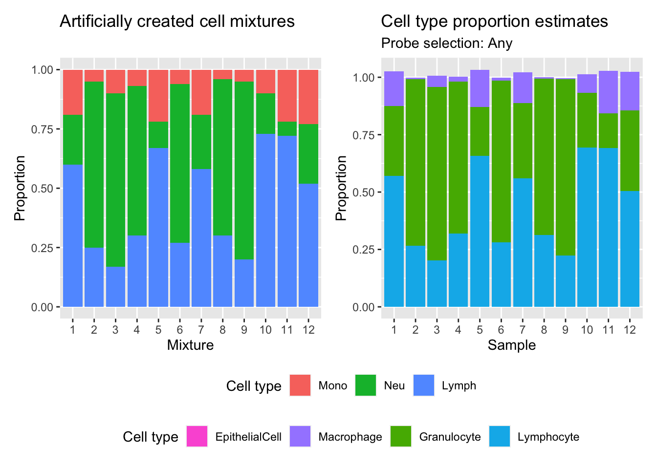
| Version | Author | Date |
|---|---|---|
| 1add90b | JovMaksimovic | 2020-07-31 |
We can see that the estimates of granulocyte and lymphocute proportions made using our BAL reference panel are highly correlated with the true proportions regardless of how the discrimination probe set is chosen. Although there is evidence of slight overestimation of granulocytes in some samples. For example, mixtures 1, 5, 7, 10, 11 and 12 are dominated by >50% lymphocytes and in those samples the proportion of granulocytes is slightly overestimated. This discrepancy is likely due to the fact that the mixture samples contain only neutrophils whearas our refernce panel contains all granulocyte types. However, despite this shortcoming, the cell type proportion estimates are still very accurate. This suggests that our BAL reference panel, in combination with the Houseman algorithm, should be able to accurately estimate cell type proportions in our patient BAL samples.
dat1 <- tibble(x = rowMeans(cbind(mixSum[,"Neu"],
                                 mixEstAny$counts[,"Granulocyte"])),
              y = (mixSum[,"Neu"] - mixEstAny$counts[,"Granulocyte"]))
c1 <- cor.test(mixSum[,'Neu'], mixEstAny$counts[,'Granulocyte'])
p1 <- ggplot(dat1, aes(x = x, y = y)) +
  geom_text(label = 1:nrow(mixSum), size = 3) +
  geom_hline(yintercept = 0, linetype = "dashed", colour = "red") +
  labs(x = "Mean", y = "Difference (Truth - Estimate)") +
  coord_cartesian(ylim = c(-0.2, 0.2)) +
  ggtitle("Granulocytes", subtitle = "Probe selection: Any") +
  annotate("text", x = 0.1, y = 0.15, hjust = 0, size = 3,
           label = glue::glue("Pearson correlation = {round(c1$estimate, 4)}
                               p-value = {signif(c1$p.value, 4)}"))


dat2 <- tibble(x = rowMeans(cbind(mixSum[,"Lymph"],
                                 mixEstAny$counts[,"Lymphocyte"])),
              y = (mixSum[,"Lymph"] - mixEstAny$counts[,"Lymphocyte"]))
c2 <- cor.test(mixSum[,'Lymph'], mixEstAny$counts[,'Lymphocyte'])
p2 <- ggplot(dat2, aes(x = x, y = y)) +
  geom_text(label = 1:nrow(mixSum), size = 3) +
  geom_hline(yintercept = 0, linetype = "dashed", colour = "red") +
  labs(x = "Mean", y = "Difference (Truth - Estimate)") +
  coord_cartesian(ylim = c(-0.2, 0.2)) +
  ggtitle("Lymphocytes", subtitle = "Probe selection: Any") +
  annotate("text", x = 0.1, y = 0.15, hjust = 0, size = 3,
           label = glue::glue("Pearson correlation = {round(c2$estimate, 4)}
                               p-value = {signif(c2$p.value, 4)}"))

dat3 <- tibble(x = rowMeans(cbind(mixSum[,"Neu"],
                                 mixEstBoth$counts[,"Granulocyte"])),
              y = (mixSum[,"Neu"] - mixEstBoth$counts[,"Granulocyte"]))
c3 <- cor.test(mixSum[,'Neu'], mixEstBoth$counts[,'Granulocyte'])
p3 <- ggplot(dat3, aes(x = x, y = y)) +
  geom_text(label = 1:nrow(mixSum), size = 3) +
  geom_hline(yintercept = 0, linetype = "dashed", colour = "red") +
  labs(x = "Mean", y = "Difference (Truth - Estimate)") +
  coord_cartesian(ylim = c(-0.2, 0.2)) +
  ggtitle("Granulocytes", subtitle = "Probe selection: Both") +
  annotate("text", x = 0.1, y = 0.15, hjust = 0, size = 3,
           label = glue::glue("Pearson correlation = {round(c3$estimate, 4)}
                               p-value = {signif(c3$p.value, 4)}"))

dat4 <- tibble(x = rowMeans(cbind(mixSum[,"Lymph"],
                                 mixEstBoth$counts[,"Lymphocyte"])),
              y = (mixSum[,"Lymph"] - mixEstBoth$counts[,"Lymphocyte"]))
c4 <- cor.test(mixSum[,'Lymph'], mixEstBoth$counts[,'Lymphocyte'])
p4 <- ggplot(dat4, aes(x = x, y = y)) +
  geom_text(label = 1:nrow(mixSum), size = 3) +
  geom_hline(yintercept = 0, linetype = "dashed", colour = "red") +
  labs(x = "Mean", y = "Difference (Truth - Estimate)") +
  coord_cartesian(ylim = c(-0.2, 0.2)) +
  ggtitle("Lymphocytes", subtitle = "Probe selection: Both") +
  annotate("text", x = 0.1, y = 0.15, hjust = 0, size = 3,
           label = glue::glue("Pearson correlation = {round(c4$estimate, 4)}
                               p-value = {signif(c4$p.value, 4)}"))

(p1 | p2) / (p3 | p4)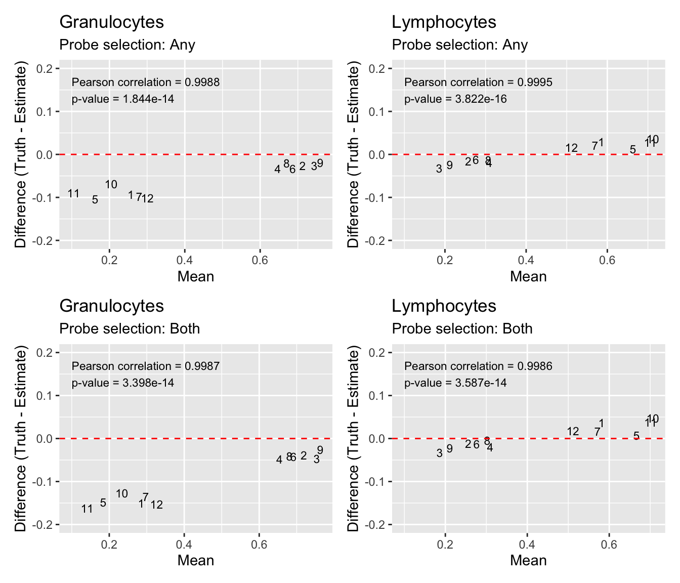
| Version | Author | Date |
|---|---|---|
| 1add90b | JovMaksimovic | 2020-07-31 |
If we look at MDS plots of the mixture data, as well as of the known cell type proportions, we can see that the primary source of variation is the proportion of neutrophils vs. lymphoctes. This overlaps with the the samples where we are seeing slight over estimation of granulocyte proportions.
mSetTargets <- preprocessRaw(RGsetTargets)
mValsTargets <- getM(mSetTargets)

mds <- plotMDS(mValsTargets, top = 1000, gene.selection = "common",
               plot = FALSE)
dat <- tibble(x = mds$x, y = mds$y, sample = 1:12)
p1 <- ggplot(dat, aes(x = x, y = y)) +
  geom_text(aes(label = sample)) +
  labs(x = "Principal Component 1", y = "Principal Component 2")

mds <- plotMDS(mixReal, top = 1000, gene.selection = "common",
               plot = FALSE)
dat <- tibble(x = mds$x, y = mds$y, sample = colnames(mixReal))
p2 <- ggplot(dat, aes(x = x, y = y)) +
  geom_text(aes(label = sample)) +
  labs(x = "Principal Component 1", y = "Principal Component 2")

(p1 | p2)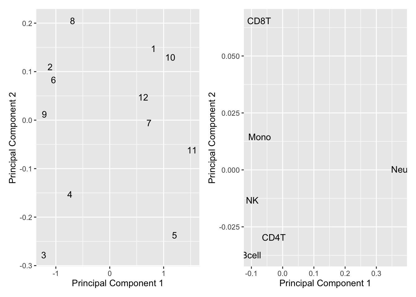
| Version | Author | Date |
|---|---|---|
| 1add90b | JovMaksimovic | 2020-07-31 |
Estimate cell type proportions in patient samples
Nine year old cohort
We can estimate the proportions of cell types in each of our patients samples using our reference panel. To select the most informative cell type probes from our reference panel we can either set the 'probeSelect paremeter to both, which selects an equal number (50) of probes (with F-stat p-value < 1E-8) with the greatest magnitude of effect from the hyper and hypo methylated sides; or any, which selects the 100 probes (with F-stat p-value < 1E-8) with the greatest magnitude of difference regardless of direction of effect.
Get estimates for proportion of each cell type using the any option.
patientSamps <- rgSet[, patients & targets$Sample_run == "Old"]
sampleNames(patientSamps) <- targets$Sample_source[patients &
                                                   targets$Sample_run == "Old"]
cellEstAny <- estimateCellCounts2(rgSet = patientSamps,
                                  compositeCellType = "Lavage",
                                  processMethod = "preprocessQuantile",
                                  probeSelect = "any",
                                  cellTypes = unique(targets$Sample_Group[cells]),
                                  referencePlatform =
                                    "IlluminaHumanMethylationEPIC",
                                  referenceset = "lavageRef",
                                  IDOLOptimizedCpGs = NULL,
                                  returnAll = TRUE,
                                  meanPlot = FALSE,
                                  keepProbes = rownames(mValsNoXY))
cellEstAny$counts
EpithelialCell Macrophage Granulocyte Lymphocyte
57G 2.918003e-02 0.73825924 0.1296844 0.11788776
37H 2.727610e-02 0.65594833 0.2637901 0.06935521
23E12 1.161119e-01 0.39439108 0.4046325 0.13196860
08F 1.111695e-01 0.40243880 0.3834029 0.14163681
54F12 7.690635e-02 0.66283168 0.1844895 0.09534994
89C 6.893183e-02 0.00000000 0.8480164 0.08981755
55F12 1.917995e-02 0.72993982 0.2008165 0.06475323
32G 3.818357e-02 0.23983986 0.6526901 0.08315512
06F 1.676799e-01 0.44776504 0.2638231 0.15538053
14G 9.683805e-02 0.64780211 0.2315210 0.04511141
12F11 2.013937e-01 0.51635765 0.2071454 0.12256490
50G 5.080749e-02 0.03095464 0.9067706 0.01994787
52H 7.474102e-02 0.15153784 0.4008492 0.39080787
62H 1.333452e-01 0.20195353 0.4985762 0.19676806
26G 2.174980e-01 0.60281464 0.1650005 0.05243131
61G 3.028481e-02 0.40250283 0.4481103 0.15011210
53F 3.824523e-02 0.11925971 0.6937976 0.17002782
41G 5.605973e-02 0.37566774 0.4233558 0.16385841
48i 1.172317e-01 0.53700706 0.3071721 0.07365130
25G12 8.045514e-02 0.54995346 0.3205317 0.07973576
45G 1.223276e-01 0.53970839 0.2749809 0.09980423
18H12 9.507074e-02 0.48938222 0.3603694 0.09003255
29G 7.020182e-02 0.51934449 0.2062113 0.21602327
M1C005F 8.673617e-19 0.09017708 0.8455570 0.07019602
21E 1.142280e-01 0.57838948 0.2109481 0.12522638
04G11 5.039341e-02 0.05935250 0.7967767 0.10825872
76B10 2.536368e-02 0.47502804 0.1540035 0.36773406
78B10 8.546334e-02 0.16715660 0.4351931 0.34376093
008G 7.390991e-02 0.08143118 0.8159434 0.06220453estAny <- reshape2::melt(cellEstAny$counts)
colnames(estAny) <- c("sample","cell","proportion")
p1 <- ggplot(estAny, aes(x = sample, fill = cell)) +
geom_bar(aes(weight = proportion)) +
ggtitle("Cell type proportion estimates",
subtitle = "Probe selection: Any") +
labs(x = "Sample", y = "Proportion", fill = "Cell type") +
theme(axis.text.x = element_text(angle = 45, hjust = 1)) +
scale_fill_manual(values = pal)
p1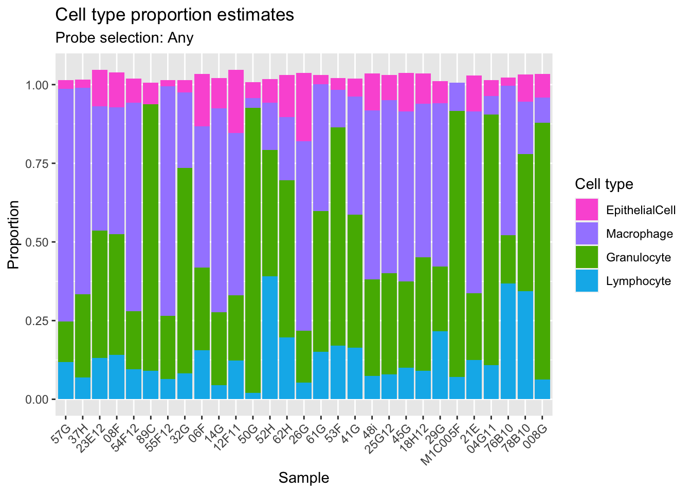
Get estimates for proportion of each cell type using the both option.
cellEstBoth <- estimateCellCounts2(rgSet = patientSamps,
                                   compositeCellType = "Lavage",
                                   processMethod = "preprocessQuantile",
                                   probeSelect = "both",
                                   cellTypes = unique(targets$Sample_Group[cells]),
                                   referencePlatform =
                                     "IlluminaHumanMethylationEPIC",
                                   referenceset = "lavageRef",
                                   IDOLOptimizedCpGs = NULL,
                                   returnAll = TRUE,
                                   meanPlot = FALSE,
                                   keepProbes = rownames(mValsNoXY))
cellEstBoth$counts
EpithelialCell Macrophage Granulocyte Lymphocyte
57G 0.02718945 0.76874278 0.1303299 0.09965848
37H 0.02567918 0.67014087 0.2618239 0.05951488
23E12 0.10883450 0.39520292 0.4252982 0.12103882
08F 0.10131180 0.42145767 0.3982569 0.12842508
54F12 0.06910058 0.69080093 0.1802139 0.08808300
89C 0.06445124 0.00000000 0.8722459 0.08209383
55F12 0.01847933 0.74086466 0.1922392 0.06285609
32G 0.03215932 0.25442217 0.6640937 0.07255313
06F 0.15833018 0.47995289 0.2635540 0.14385803
14G 0.07994141 0.68056485 0.2248303 0.04342788
12F11 0.18551269 0.54252245 0.1978467 0.12566349
50G 0.04290581 0.02950078 0.9126667 0.02319942
52H 0.07484464 0.16098805 0.4417636 0.36194400
62H 0.12660877 0.21465734 0.5251756 0.18146137
26G 0.19905524 0.63041989 0.1516000 0.05828798
61G 0.02758430 0.42533827 0.4555929 0.13434876
53F 0.04192527 0.11985814 0.7151305 0.15260829
41G 0.04885728 0.40276298 0.4316768 0.14803213
48i 0.10460212 0.56048663 0.3025526 0.07185651
25G12 0.07252395 0.55079113 0.3380054 0.07156997
45G 0.11005552 0.56381732 0.2801806 0.08950061
18H12 0.08355441 0.50445042 0.3676546 0.08233018
29G 0.06050539 0.56217195 0.2111849 0.19698441
M1C005F 0.00000000 0.09012010 0.8605841 0.05971640
21E 0.10331023 0.60795568 0.2128945 0.11480677
04G11 0.04954202 0.06491760 0.8122429 0.09823125
76B10 0.03645425 0.50802027 0.1599253 0.33448888
78B10 0.08522035 0.17788405 0.4619894 0.32228783
008G 0.06677315 0.06176092 0.8394243 0.06147165estBoth <- reshape2::melt(cellEstBoth$counts)
colnames(estBoth) <- c("sample","cell","proportion")
p2 <- ggplot(estBoth, aes(x = sample, fill = cell)) +
geom_bar(aes(weight = proportion)) +
ggtitle("Cell type proportion estimates",
subtitle = "Probe selection: Both") +
labs(x = "Sample", y = "Proportion", fill = "Cell type") +
theme(axis.text.x = element_text(angle = 45, hjust = 1)) +
scale_fill_manual(values = pal)
p2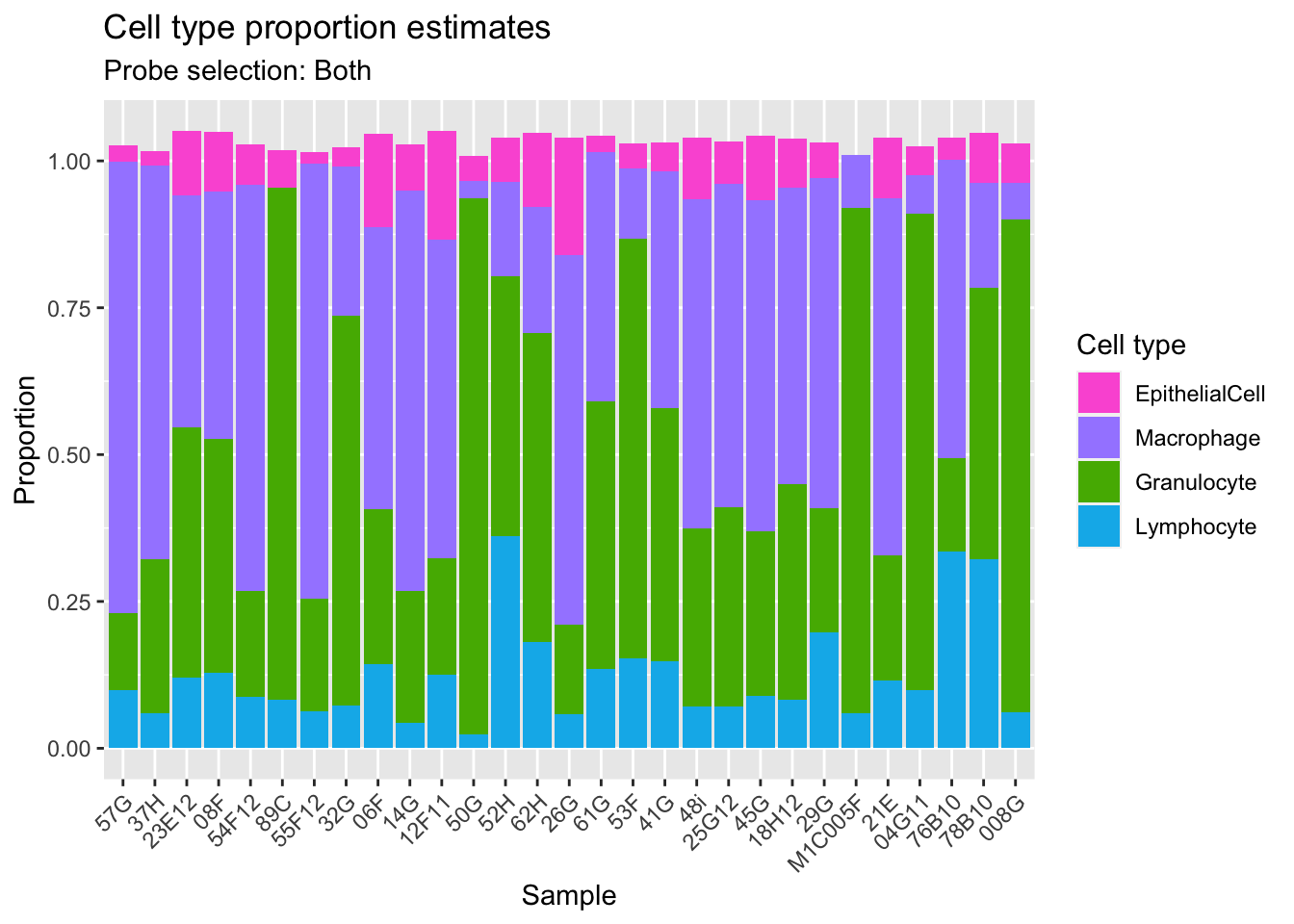
(p1 | p2) +
  plot_layout(guides = "collect") &
  theme(legend.position = "bottom",
        axis.text.x = element_text(size = 7))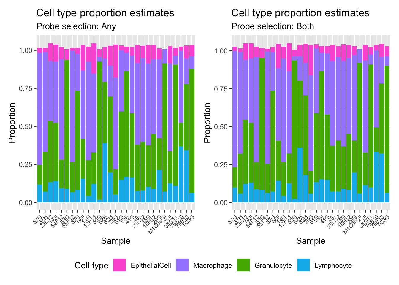
Test for case/control differences
Test whether there are any statistically significant differnces between cases and controls in the estimated proportions of the various cell types (based on estimates made using any for probe selection). Granulocytes are significantly higher in controls (FDR < 0.05) and macrophages are significantly lower (FDR < 0.05).
caseCtrl <- factor(targets$Sample_Group[patients & targets$Sample_run == "Old"])
design <- model.matrix(~caseCtrl)

fit <- lmFit(t(cellEstAny$counts), design)
fit <- eBayes(fit)

t1 <- topTable(fit)
Removing intercept from test coefficientst1 logFC AveExpr t P.Value adj.P.Val
Granulocyte 0.27702453 0.4149710 3.846312 0.0006079233 0.002431693
Macrophage -0.20793171 0.3933516 -2.785427 0.0093319443 0.018663889
EpithelialCell -0.03276043 0.0823613 -1.619258 0.1162412683 0.154988358
Lymphocyte -0.04170882 0.1343987 -1.223302 0.2310847114 0.231084711
B
Granulocyte -0.379545
Macrophage -2.890693
EpithelialCell -5.063868
Lymphocyte -5.588982Test whether there are any statistically significant differnces between cases and controls in the estimated proportions of the various cell types (based on estimates made using both for probe selection). Granulocytes are significantly higher in controls (FDR < 0.05) and macrophages are significantly lower (FDR < 0.05).
fit <- lmFit(t(cellEstBoth$counts), design)
fit <- eBayes(fit)

t2 <- topTable(fit)
Removing intercept from test coefficientst2 logFC AveExpr t P.Value adj.P.Val
Granulocyte 0.28569991 0.42382681 3.836071 0.0006317574 0.002527029
Macrophage -0.22044905 0.40967496 -2.837116 0.0082671467 0.016534293
EpithelialCell -0.03225433 0.07604525 -1.770522 0.0872695510 0.116359401
Lymphocyte -0.03982494 0.12380342 -1.273875 0.2129338788 0.212933879
B
Granulocyte -0.411715
Macrophage -2.777812
EpithelialCell -4.828628
Lymphocyte -5.526241Plot cell type proportion estimates stratified by patient status. There are statistically significant differences between cases and controls in the proportions of granulocytes and macrophages, in particular.
estAny$status <- rep(targets$Sample_Group[patients &
                                            targets$Sample_run == "Old"],
                     length(unique(estAny$cell)))

a <- ggplot(estAny, aes(x=cell, y=proportion, fill=status)) +
  geom_boxplot() +
  geom_jitter(position = position_dodge(0.75), alpha = 0.5) +
  labs(y="Estimated proportion", x="Cell type", fill="Status") +
  ggtitle("Probe selection: Any") +
  annotate("text", x = 2, y = 0.825, size = 3,
           label = glue("*Adj. p-val = {round(t1['Macrophage',]$adj.P.Val, 4)}")) +
  annotate("text", x = 3, y = 0.95, size = 3,
           label = glue("*Adj. p-val = {round(t1['Granulocyte',]$adj.P.Val, 4)}"))

estBoth$status <- rep(targets$Sample_Group[patients &
                                            targets$Sample_run == "Old"],
                     length(unique(estBoth$cell)))

b <- ggplot(estBoth, aes(x=cell, y=proportion, fill=status)) +
  geom_boxplot() +
  geom_jitter(position = position_dodge(0.75), alpha = 0.5) +
  labs(y="Estimated proportion", x="Cell type", fill="Status") +
  ggtitle("Probe selection: Both") +
  annotate("text", x = 2, y = 0.85, size = 3,
           label = glue("*Adj. p-val = {round(t2['Macrophage',]$adj.P.Val, 4)}")) +
  annotate("text", x = 3, y = 0.975, size = 3,
           label = glue("*Adj. p-val = {round(t2['Granulocyte',]$adj.P.Val, 4)}"))

(a | b) + plot_layout(guides = "collect") & theme(legend.position = "bottom")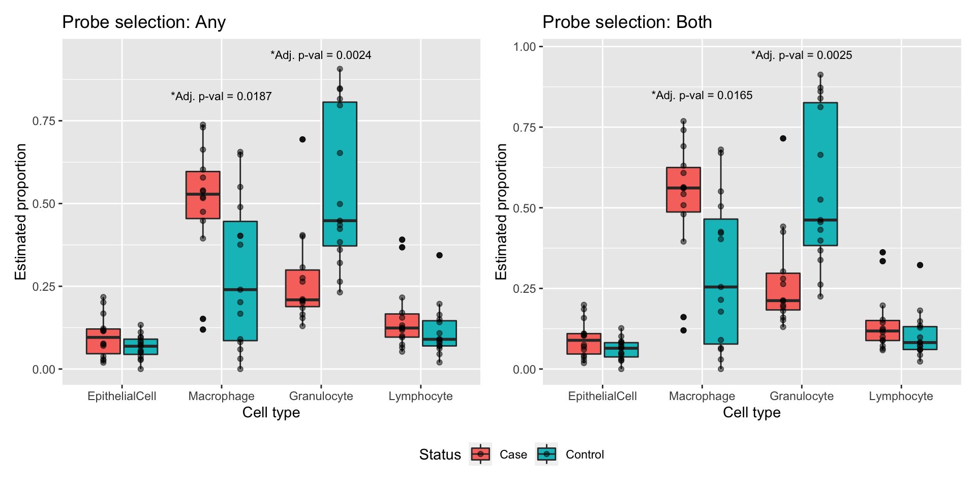
Five year old cohort
We can estimate the proportions of cell types in each of our patients samples using our reference panel. To select the most informative cell type probes from our reference panel we can either set the 'probeSelect paremeter to both, which selects an equal number (50) of probes (with F-stat p-value < 1E-8) with the greatest magnitude of effect from the hyper and hypo methylated sides; or any, which selects the 100 probes (with F-stat p-value < 1E-8) with the greatest magnitude of difference regardless of direction of effect.
Get estimates for proportion of each cell type using the any option.
patientSamps <- rgSet[, patients & targets$Sample_run == "New"]
sampleNames(patientSamps) <- targets$Sample_source[patients &
                                                   targets$Sample_run == "New"]
cellEstAny <- estimateCellCounts2Mod(rgSet = patientSamps,
                                  compositeCellType = "Lavage",
                                  processMethod = "preprocessQuantile",
                                  probeSelect = "any",
                                  cellTypes = unique(targets$Sample_Group[cells]),
                                  referencePlatform =
                                    "IlluminaHumanMethylationEPIC",
                                  referenceset = "lavageRef",
                                  IDOLOptimizedCpGs = NULL,
                                  returnAll = TRUE,
                                  meanPlot = FALSE,
                                  keepProbes = rownames(mValsNoXY))
cellEstAny$counts
EpithelialCell Macrophage Granulocyte Lymphocyte
CF4 0.09887811 0.665870284 0.1373721575 0.11591448
CF1 0.09160594 0.007008491 0.8876070762 0.01582198
CF3 0.21008393 0.373080727 0.2205069746 0.22332255
CF2 0.11202740 0.299187291 0.4306758485 0.19700599
CF5 0.05604734 0.506830829 0.3446874744 0.11035638
Control 0.12888375 0.137396548 0.5865391861 0.17772693
M1C085b11 0.09834150 0.847236099 0.0244369404 0.03816931
M1C074b10 0.13176362 0.795413428 0.0357311834 0.04772542
M1C107b13 0.15866381 0.312517901 0.2304719548 0.33393213
M1C086c11 0.04190740 0.900779906 0.0040188837 0.05287329
M1C059c09 0.18337260 0.621697749 0.1439821241 0.07039921
M1C108b13 0.06350874 0.848066306 0.0460810089 0.04777036
P1C195b13 0.10657932 0.833444504 0.0000000000 0.06737140
P1C171b11 0.37030667 0.603514252 0.0443810392 0.02051106
P1C132b09 0.32556868 0.338059879 0.1111998186 0.25193011
P1C139c09 0.05128893 0.616897647 0.2621834812 0.09125539
P1C141b09 0.23370792 0.574703880 0.1480189365 0.07197363
P1C174a11 0.55055645 0.319575459 0.0387785331 0.13954888
P1C152b10 0.24222503 0.703933452 0.0464024664 0.03167612
M1C077b10 0.09976434 0.674425243 0.1442296535 0.09347002
M1C073b10 0.09842319 0.734380334 0.1133559109 0.06459183
M1C081b10 0.16285972 0.265825345 0.4095456302 0.20713566
M1C075b10 0.03099690 0.254170680 0.6592864708 0.07250104
M1C079b10 0.27619526 0.291391155 0.1832794979 0.27831544
M1C100b12 0.37503845 0.483558074 0.1072887643 0.07116257
M1C122c14 0.29431949 0.539265174 0.0209690170 0.15461282
P1C192b13 0.05627938 0.470244616 0.3989282724 0.09492746
P1C167b11 0.16252703 0.685639703 0.0251019565 0.13644935
P1C185b12 0.15949914 0.207396112 0.5120003361 0.14116505
P1C165a10 0.07920254 0.864213917 0.0193187757 0.04000526
P1C187b12 0.06510918 0.798614807 0.0880340459 0.05605912
P1C166b11 0.12540786 0.149785485 0.6870799504 0.06281179
P1C176b11 0.38957108 0.203887134 0.1541761366 0.29069268
P1C182b12 0.36234004 0.424124350 0.0008761498 0.20818021
M1C111b13 0.20240365 0.423114797 0.2751150379 0.16691892
M1C123b14 0.05190977 0.846052836 0.0724897576 0.03588586
M1C113b13 0.17179293 0.573524902 0.1936136608 0.10229028
M1C125b14 0.31006230 0.478671615 0.1108757586 0.13090659
M1C127b14 0.17689391 0.458195600 0.3534693643 0.05406513
M1C109b13 0.27746313 0.487360758 0.1650461912 0.11257758
M1C129b14 0.18383250 0.347589837 0.2815669476 0.21501265
M1C117b14 0.07885942 0.386525718 0.3913356105 0.15408518
P1C193b13 0.40870354 0.364328156 0.2911832231 0.00000000
P1C178b11 0.19201489 0.729101131 0.0004817958 0.08758004
P1C180b12 0.43787166 0.238181848 0.2173612927 0.14190221
P1C213b14 0.17688806 0.507425057 0.2704583133 0.07493587
P1C183b12 0.13024478 0.724388027 0.1029432167 0.06454139
P1C170b11 0.35621040 0.437406371 0.1798887767 0.06359025
P1C210b14 0.10609303 0.755803229 0.0222984590 0.11716206
P1C161b10 0.15769304 0.437278820 0.4000225975 0.03401306
P1C169b11 0.19247482 0.177571537 0.6046560888 0.05552079
P1C163a09 0.20158877 0.556884845 0.0329312997 0.22161017
P1C184b12 0.14291289 0.555061722 0.2115101477 0.12915261
M1C126b14 0.43033109 0.414374844 0.0748600125 0.11340837
P1C188b12 0.26610401 0.704053050 0.0283152113 0.02719808
P1C224a14 0.14837035 0.255982333 0.5535079157 0.07440791
P1C201b13 0.25975622 0.635245765 0.0359261789 0.09219751
P1C140b09 0.04625600 0.782687361 0.1125381464 0.06423774
P1C134b09 0.11353162 0.223045558 0.5633578870 0.12326478
P1C156b10 0.15831955 0.604717108 0.0675720564 0.19080876
P1C159b10 0.15292211 0.539315176 0.2122733702 0.13918655
P1C136b09 0.13683760 0.473176007 0.2452274431 0.15972858estAny <- reshape2::melt(cellEstAny$counts)
colnames(estAny) <- c("sample","cell","proportion")
p1 <- ggplot(estAny, aes(x = sample, fill = cell)) +
geom_bar(aes(weight = proportion)) +
ggtitle("Cell type proportion estimates",
subtitle = "Probe selection: Any") +
labs(x = "Sample", y = "Proportion", fill = "Cell type") +
theme(axis.text.x = element_text(angle = 45, hjust = 1, size = 7),
legend.position = "bottom") +
scale_fill_manual(values = pal)
p1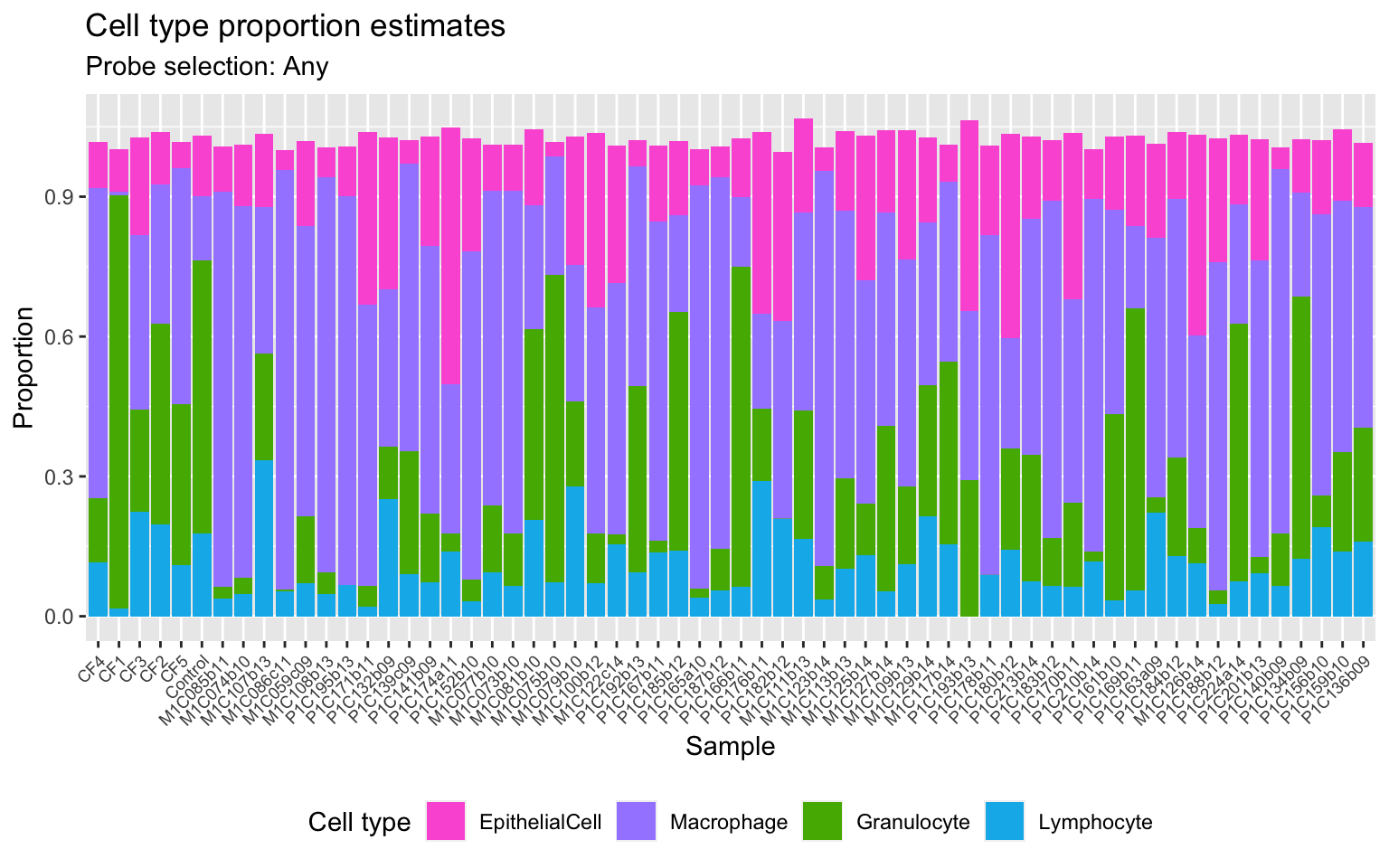
Get estimates for proportion of each cell type using the both option.
cellEstBoth <- estimateCellCounts2Mod(rgSet = patientSamps,
                                   compositeCellType = "Lavage",
                                   processMethod = "preprocessQuantile",
                                   probeSelect = "both",
                                   cellTypes = unique(targets$Sample_Group[cells]),
                                   referencePlatform =
                                     "IlluminaHumanMethylationEPIC",
                                   referenceset = "lavageRef",
                                   IDOLOptimizedCpGs = NULL,
                                   returnAll = TRUE,
                                   meanPlot = FALSE,
                                   keepProbes = rownames(mValsNoXY))
cellEstBoth$counts
EpithelialCell Macrophage Granulocyte Lymphocyte
CF4 0.09704272 0.685925133 0.15400581 0.09967193
CF1 0.08698901 0.004624043 0.89762350 0.01759464
CF3 0.20029882 0.392829903 0.25700053 0.20678557
CF2 0.10544363 0.336904993 0.48004548 0.16317052
CF5 0.05406218 0.527821375 0.35682666 0.09496959
Control 0.12786563 0.130576604 0.61730116 0.16658208
M1C085b11 0.09268689 0.874845438 0.02168849 0.03063821
M1C074b10 0.12387793 0.825207456 0.03204921 0.04242311
M1C107b13 0.14670229 0.395420274 0.30407237 0.27679425
M1C086c11 0.03679955 0.935454247 0.00599981 0.03689651
M1C059c09 0.17251035 0.630231278 0.16042844 0.06839581
M1C108b13 0.05800535 0.867006251 0.05563173 0.03966513
P1C195b13 0.10110008 0.867341618 0.00000000 0.05663398
P1C171b11 0.34708538 0.641372279 0.01912608 0.03768792
P1C132b09 0.31134281 0.373651990 0.12943744 0.24317256
P1C139c09 0.05127804 0.620954367 0.27435956 0.08414116
P1C141b09 0.21910699 0.596837927 0.15285129 0.07422140
P1C174a11 0.52311345 0.356564531 0.03377541 0.15423879
P1C152b10 0.22728294 0.727107934 0.03685607 0.04134041
M1C077b10 0.09690015 0.671289033 0.15669384 0.09239905
M1C073b10 0.09588902 0.739184945 0.11553907 0.06455059
M1C081b10 0.14430751 0.321964001 0.49240649 0.15758698
M1C075b10 0.03192684 0.260092970 0.67263339 0.06036425
M1C079b10 0.23881426 0.395548824 0.29978934 0.21363442
M1C100b12 0.34367398 0.524919491 0.12943906 0.07478366
M1C122c14 0.24425899 0.645519065 0.09462553 0.12014788
P1C192b13 0.05242408 0.486758155 0.41431922 0.08245620
P1C167b11 0.14869959 0.724199084 0.05218966 0.11987293
P1C185b12 0.14664302 0.227247170 0.55037296 0.12504619
P1C165a10 0.07259057 0.880016096 0.03397341 0.03210254
P1C187b12 0.06522757 0.809249970 0.09866926 0.04375206
P1C166b11 0.11768748 0.152258006 0.70858337 0.05672472
P1C176b11 0.37202162 0.210484610 0.23193037 0.26898028
P1C182b12 0.31075479 0.541767318 0.09370076 0.15994039
M1C111b13 0.17169551 0.480611999 0.34814989 0.13508797
M1C123b14 0.04858126 0.850257501 0.08610770 0.02955360
M1C113b13 0.15877812 0.613279325 0.21295138 0.08349076
M1C125b14 0.26892870 0.557158889 0.17676469 0.10295058
M1C127b14 0.16224334 0.473755246 0.36405622 0.05336221
M1C109b13 0.23489088 0.556342177 0.22309362 0.09372095
M1C129b14 0.16807306 0.409891662 0.34234827 0.17247265
M1C117b14 0.07407313 0.396003480 0.41967665 0.13928640
P1C193b13 0.37928920 0.383570988 0.29417114 0.01870840
P1C178b11 0.17970626 0.757037542 0.00000000 0.08691815
P1C180b12 0.39996258 0.291030474 0.27036876 0.13163302
P1C213b14 0.16239169 0.523860433 0.29742092 0.06531109
P1C183b12 0.12370603 0.758888568 0.10116107 0.05259922
P1C170b11 0.33454706 0.453220016 0.19399958 0.07140840
P1C210b14 0.10266031 0.770251410 0.02739993 0.11074308
P1C161b10 0.14684100 0.453158213 0.40208578 0.03510941
P1C169b11 0.17976824 0.178035979 0.61926679 0.06062221
P1C163a09 0.17778416 0.645680115 0.11523259 0.16111714
P1C184b12 0.13738309 0.547324323 0.23666908 0.12329291
M1C126b14 0.39802995 0.476387362 0.09000109 0.11238789
P1C188b12 0.24521268 0.731511194 0.02805627 0.03234504
P1C224a14 0.13879279 0.261433006 0.57579663 0.06921504
P1C201b13 0.24738843 0.661866282 0.02095522 0.09795828
P1C140b09 0.04417380 0.805924948 0.11861423 0.05099715
P1C134b09 0.11084952 0.228142809 0.58874589 0.11249551
P1C156b10 0.13593947 0.678204104 0.14107498 0.14287367
P1C159b10 0.14396176 0.538912418 0.24041581 0.13051632
P1C136b09 0.13273237 0.498370514 0.26408110 0.14445619estBoth <- reshape2::melt(cellEstBoth$counts)
colnames(estBoth) <- c("sample","cell","proportion")
p2 <- ggplot(estBoth, aes(x = sample, fill = cell)) +
geom_bar(aes(weight = proportion)) +
ggtitle("Cell type proportion estimates",
subtitle = "Probe selection: Both") +
labs(x = "Sample", y = "Proportion", fill = "Cell type") +
theme(axis.text.x = element_text(angle = 45, hjust = 1, size = 7),
legend.position = "bottom") +
scale_fill_manual(values = pal)
p2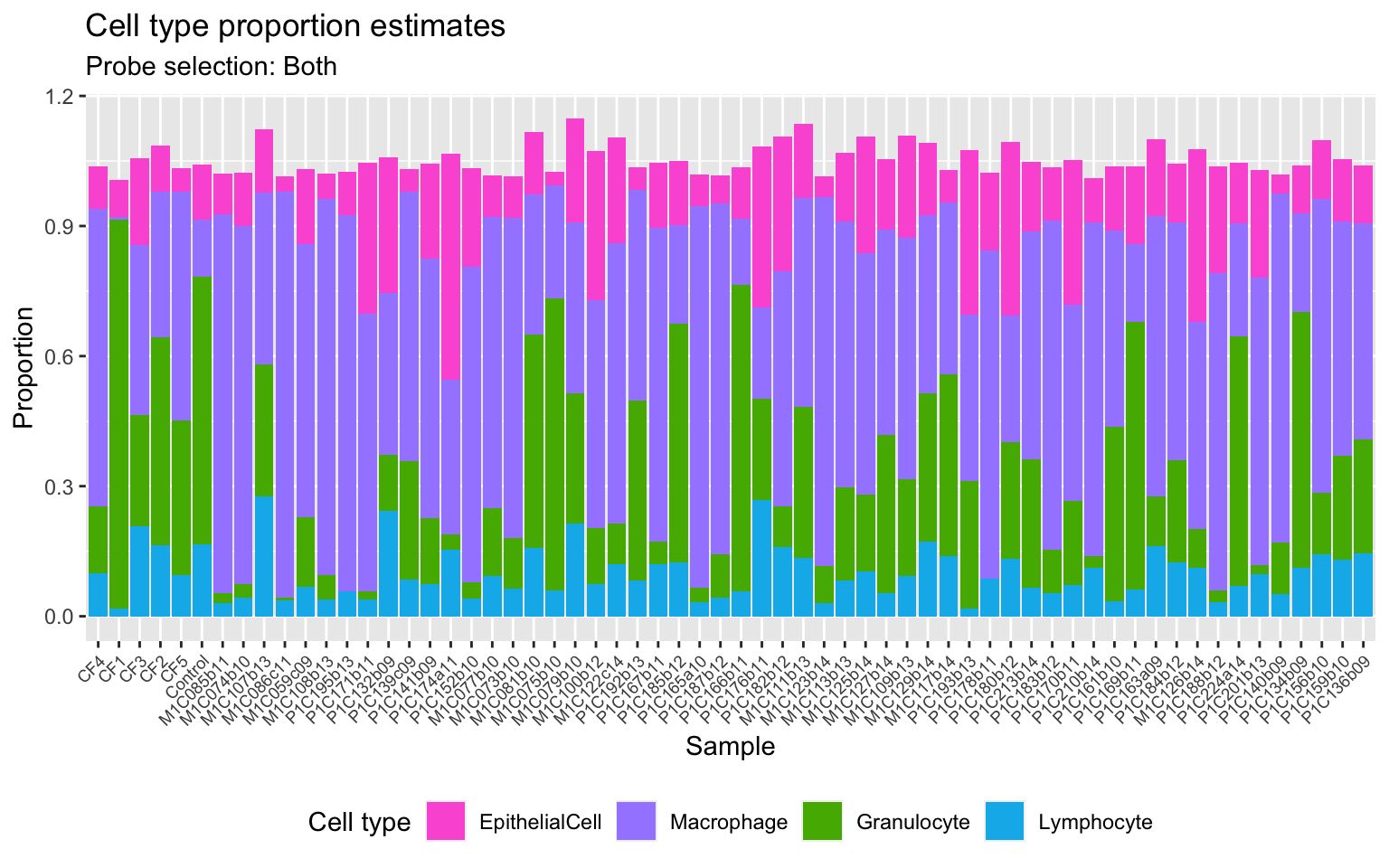
(p1 / p2) +
  plot_layout(guides = "collect") &
  theme(legend.position = "bottom",
        axis.text.x = element_text(size = 7))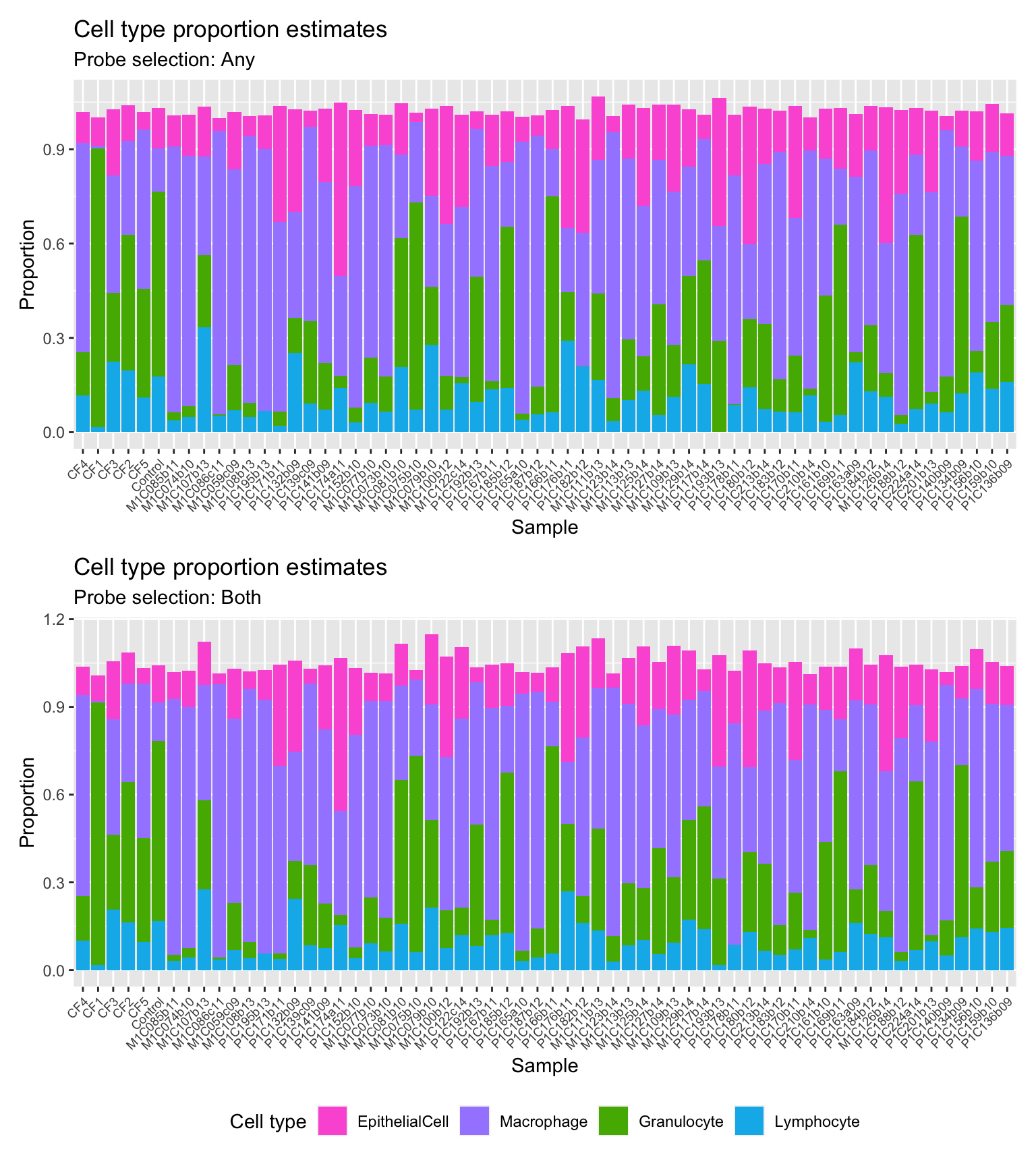
Compare to flow-cytometry data
samps <- targets$Sample_source[targets$Sample_Group == "Raw"]
melt(read.csv(here("data/Flow-Data-for-Reference-Panel-Scaled.csv"),
              stringsAsFactors = FALSE)) %>%
  inner_join(melt(read.csv(here("data/Flow-Data-for-Reference-Panel-Original.csv"),
                           stringsAsFactors = FALSE)),
             by = c("X", "variable")) %>%
  rename(cell = X,
         sample = variable,
         scaled = value.x,
         original = value.y) %>%
  mutate(scaled = scaled / 100,
         original = original / 100) %>%
  inner_join(estBoth[estBoth$sample %in% samps,] %>%
               rename(both = proportion) %>%
               inner_join(estAny[estBoth$sample %in% samps,] %>%
                            rename(any = proportion))  %>%
               mutate(cell = gsub("EpithelialCell","AEC", cell),
                      cell = gsub("Macrophage","macrophages", cell),
                      cell = gsub("Granulocyte","granulocytes", cell),
                      cell = gsub("Lymphocyte","lymphocytes", cell))) %>%
  pivot_longer(cols = c(scaled, original)) -> dat

p1 <- ggplot(dat, aes(x = rowMeans(cbind(value, any)),
                      y = value - any, colour = cell)) +
  geom_point(aes(shape = name)) +
  geom_hline(yintercept = 0, linetype = "dashed", colour = "red") +
  facet_wrap(vars(sample), ncol = 3, nrow = 2) +
  labs(x = "Mean", y = "Difference (Flow - Meth. est.)",
       colour = "Cell Type", shape = "Flow Data") +
  scale_shape_manual(values = c(1,4)) +
  ggtitle("Probe selection: Any")

p2 <- ggplot(dat, aes(x = rowMeans(cbind(value, both)),
                      y = value - both, colour = cell)) +
  geom_point(aes(shape = name)) +
  geom_hline(yintercept = 0, linetype = "dashed", colour = "red") +
  facet_wrap(vars(sample), ncol = 3, nrow = 2) +
  labs(x = "Mean", y = "Difference (Flow - Meth. est.)",
       colour = "Cell Type", shape = "Flow Data") +
  scale_shape_manual(values = c(1,4)) +
  ggtitle("Probe selection: Both")

p1 / p2 + plot_layout(guides = "collect")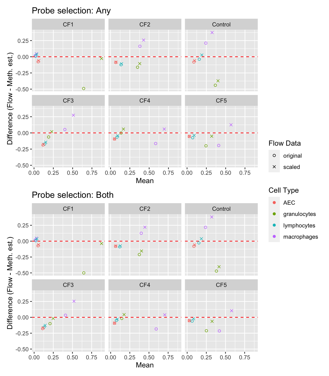
samps <- as.character(unique(dat$sample))
p <- vector("list", length(samps))

for(i in 1:length(samps)){
  dat1 <- filter(dat, sample == samps[i])
  c1 <- cor.test(dat1$any, dat1$value)
  p[[i]] <- ggplot(dat1, aes(x = rowMeans(cbind(value, any)),
                         y = value - any, colour = cell)) +
    geom_point(aes(shape = name)) +
    scale_shape_manual(values = c(1,4)) +
    geom_hline(yintercept = 0, linetype = "dashed", colour = "red") +
    labs(x = "Mean", y = "Difference (Flow - Meth. est.)",
         colour = "Cell type") +
    coord_cartesian(ylim = c(-0.5, 0.5), xlim = c(0, 1)) +
    ggtitle({samps[i]}) +
    annotate("text", x = 0, y = 0.45, hjust = 0, size = 3,
             label = glue::glue("Pearson correlation = {round(c1$estimate, 4)}
                               p-value = {signif(c1$p.value, 4)}"))

}

p1 <- wrap_plots(p, ncol = 3, guides = "collect") +
  plot_annotation(title = "Probe selection: Any") &
  theme(legend.position = "bottom", legend.box = "vertical")

for(i in 1:length(samps)){
  dat1 <- filter(dat, sample == samps[i])
  c1 <- cor.test(dat1$both, dat1$value)
  p[[i]] <- ggplot(dat1, aes(x = rowMeans(cbind(value, both)),
                         y = value - both, colour = cell)) +
    geom_point(aes(shape = name)) +
    scale_shape_manual(values = c(1,4)) +
    geom_hline(yintercept = 0, linetype = "dashed", colour = "red") +
    labs(x = "Mean", y = "Difference (Flow - Meth. est.)",
         colour = "Cell type") +
    coord_cartesian(ylim = c(-0.5, 0.5), xlim = c(0, 1)) +
    ggtitle(samps[i]) +
    annotate("text", x = 0, y = 0.45, hjust = 0, size = 3,
             label = glue::glue("Pearson correlation = {round(c1$estimate, 4)}
                               p-value = {signif(c1$p.value, 4)}"))

}

p2 <- wrap_plots(p, ncol = 3, guides = "collect") +
  plot_annotation(title = "Probe selection: Both") &
  theme(legend.position = "bottom", legend.box = "vertical")

wrap_elements(p1) /
    wrap_elements(p2)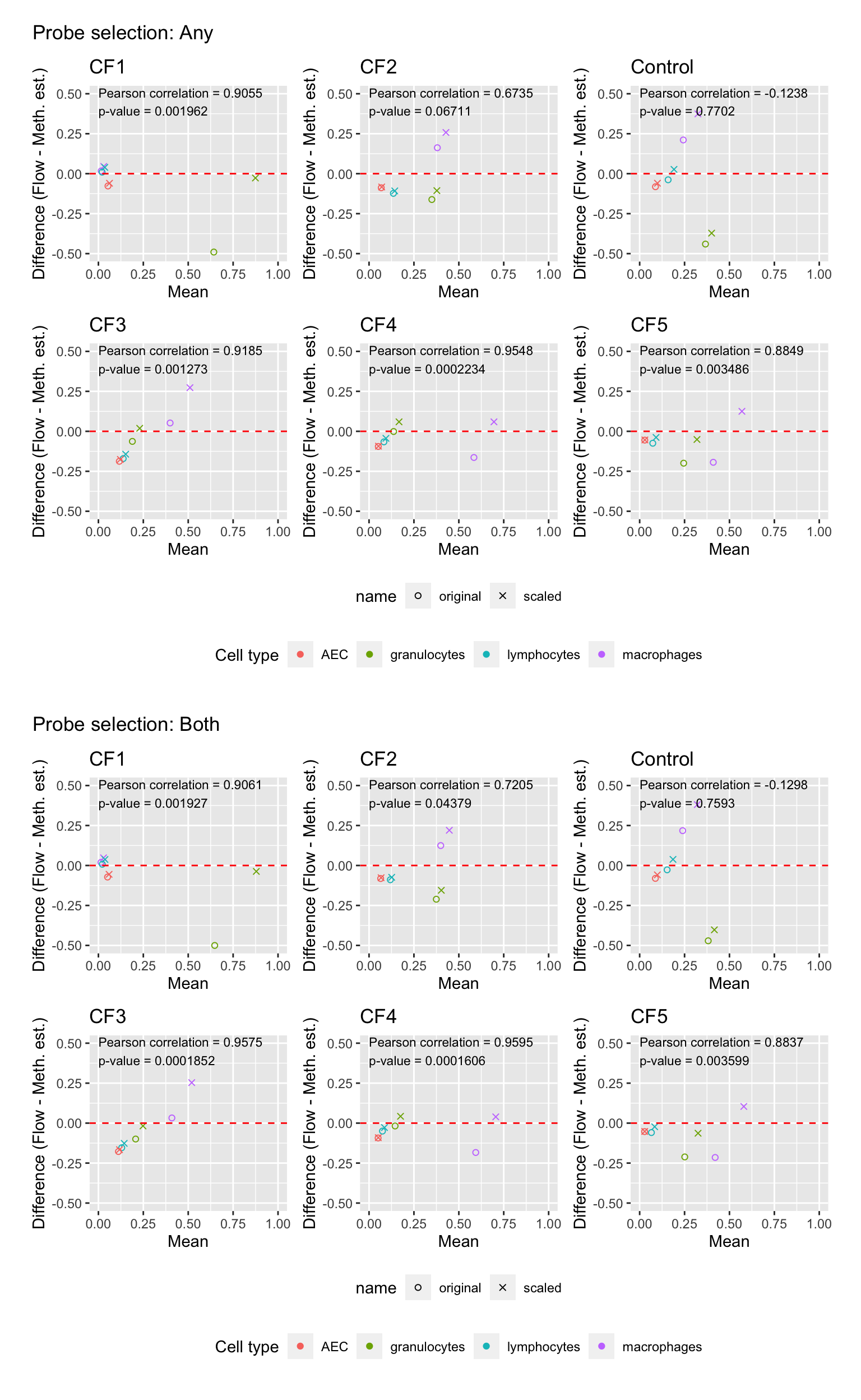
Test for case/control differences
Test whether there are any statistically significant differnces between cases and controls in the estimated proportions of the various cell types (based on estimates made using any for probe selection). No statistically significant differences between cases and controls.
caseCtrl <- factor(targets$Sample_Group[patients & targets$Sample_run == "New"])
design <- model.matrix(~caseCtrl)

fit <- lmFit(t(cellEstAny$counts), design)
fit <- eBayes(fit)

t1 <- topTable(fit, coef = "caseCtrlControl")
t1
logFC AveExpr t P.Value adj.P.Val B
Granulocyte 0.09634006 0.2151189 1.9229755 0.05907215 0.2362886 -4.151928
Macrophage -0.06548192 0.5075678 -1.1654459 0.24829604 0.3436926 -5.190440
EpithelialCell -0.03566323 0.1880838 -1.1421681 0.25776942 0.3436926 -5.214772
Lymphocyte 0.01022188 0.1132831 0.4943642 0.62279354 0.6227935 -5.699639Test whether there are any statistically significant differnces between cases and controls in the estimated proportions of the various cell types (based on estimates made using both for probe selection). No statistically significant differences between cases and controls.
fit <- lmFit(t(cellEstBoth$counts), design)
fit <- eBayes(fit)

t2 <- topTable(fit, coef = "caseCtrlControl")
t2
logFC AveExpr t P.Value adj.P.Val B
Granulocyte 0.11077298 0.2408485 2.1745568 0.0335277 0.1341108 -3.781152
EpithelialCell -0.03659298 0.1737548 -1.2809382 0.2050351 0.3507482 -5.164812
Macrophage -0.06353364 0.5380853 -1.1295515 0.2630612 0.3507482 -5.333114
Lymphocyte 0.00288474 0.1004516 0.1691252 0.8662544 0.8662544 -5.916396Plot cell type proportion estimates stratified by patient status. There are no statistically significant differences between cases and controls in the estimated proportions of cell types.
estAny$status <- rep(targets$Sample_Group[patients &
                                            targets$Sample_run == "New"],
                     length(unique(estAny$cell)))

a <- ggplot(estAny, aes(x=cell, y=proportion, fill=status)) +
  geom_boxplot() +
  geom_jitter(position = position_dodge(0.75), alpha = 0.5) +
  labs(y="Estimated proportion", x="Cell type", fill="Status") +
  ggtitle("Probe selection: Any")

estBoth$status <- rep(targets$Sample_Group[patients &
                                            targets$Sample_run == "New"],
                     length(unique(estBoth$cell)))

b <- ggplot(estBoth, aes(x=cell, y=proportion, fill=status)) +
  geom_boxplot() +
  geom_jitter(position = position_dodge(0.75), alpha = 0.5) +
  labs(y="Estimated proportion", x="Cell type", fill="Status") +
  ggtitle("Probe selection: Both")

(a | b) + plot_layout(guides = "collect") & theme(legend.position = "bottom")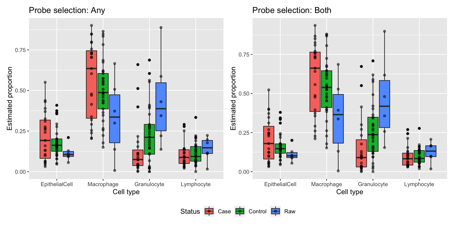
| Version | Author | Date |
|---|---|---|
| ac6a20c | JovMaksimovic | 2020-10-30 |
sessionInfo()R version 4.0.3 (2020-10-10)
Platform: x86_64-apple-darwin17.0 (64-bit)
Running under: macOS Mojave 10.14.6
Matrix products: default
BLAS: /Library/Frameworks/R.framework/Versions/4.0/Resources/lib/libRblas.dylib
LAPACK: /Library/Frameworks/R.framework/Versions/4.0/Resources/lib/libRlapack.dylib
locale:
[1] en_AU.UTF-8/en_AU.UTF-8/en_AU.UTF-8/C/en_AU.UTF-8/en_AU.UTF-8
attached base packages:
[1] stats4 parallel stats graphics grDevices utils datasets
[8] methods base
other attached packages:
[1] patchwork_1.1.1
[2] forcats_0.5.0
[3] stringr_1.4.0
[4] dplyr_1.0.2
[5] purrr_0.3.4
[6] readr_1.4.0
[7] tidyr_1.1.2
[8] tibble_3.0.4
[9] tidyverse_1.3.0
[10] reshape2_1.4.4
[11] ggplot2_3.3.2
[12] FlowSorted.Blood.EPIC_1.8.0
[13] ExperimentHub_1.16.0
[14] AnnotationHub_2.22.0
[15] BiocFileCache_1.14.0
[16] dbplyr_2.0.0
[17] nlme_3.1-151
[18] quadprog_1.5-8
[19] genefilter_1.72.0
[20] IlluminaHumanMethylationEPICmanifest_0.3.0
[21] IlluminaHumanMethylationEPICanno.ilm10b4.hg19_0.6.0
[22] minfi_1.36.0
[23] bumphunter_1.32.0
[24] locfit_1.5-9.4
[25] iterators_1.0.13
[26] foreach_1.5.1
[27] Biostrings_2.58.0
[28] XVector_0.30.0
[29] SummarizedExperiment_1.20.0
[30] Biobase_2.50.0
[31] MatrixGenerics_1.2.0
[32] matrixStats_0.57.0
[33] GenomicRanges_1.42.0
[34] GenomeInfoDb_1.26.2
[35] IRanges_2.24.1
[36] S4Vectors_0.28.1
[37] BiocGenerics_0.36.0
[38] limma_3.46.0
[39] glue_1.4.2
[40] here_1.0.1
[41] workflowr_1.6.2
loaded via a namespace (and not attached):
[1] readxl_1.3.1 backports_1.2.1
[3] plyr_1.8.6 splines_4.0.3
[5] BiocParallel_1.24.1 digest_0.6.27
[7] htmltools_0.5.0 fansi_0.4.1
[9] magrittr_2.0.1 memoise_1.1.0
[11] annotate_1.68.0 modelr_0.1.8
[13] askpass_1.1 siggenes_1.64.0
[15] prettyunits_1.1.1 colorspace_2.0-0
[17] rvest_0.3.6 blob_1.2.1
[19] rappdirs_0.3.1 haven_2.3.1
[21] xfun_0.19 jsonlite_1.7.2
[23] crayon_1.3.4 RCurl_1.98-1.2
[25] GEOquery_2.58.0 survival_3.2-7
[27] gtable_0.3.0 zlibbioc_1.36.0
[29] DelayedArray_0.16.0 Rhdf5lib_1.12.0
[31] HDF5Array_1.18.0 scales_1.1.1
[33] DBI_1.1.0 rngtools_1.5
[35] Rcpp_1.0.5 xtable_1.8-4
[37] progress_1.2.2 bit_4.0.4
[39] mclust_5.4.7 preprocessCore_1.52.0
[41] httr_1.4.2 RColorBrewer_1.1-2
[43] ellipsis_0.3.1 farver_2.0.3
[45] pkgconfig_2.0.3 reshape_0.8.8
[47] XML_3.99-0.5 labeling_0.4.2
[49] tidyselect_1.1.0 rlang_0.4.9
[51] later_1.1.0.1 AnnotationDbi_1.52.0
[53] cellranger_1.1.0 munsell_0.5.0
[55] BiocVersion_3.12.0 tools_4.0.3
[57] cli_2.2.0 generics_0.1.0
[59] RSQLite_2.2.1 broom_0.7.3
[61] evaluate_0.14 fastmap_1.0.1
[63] yaml_2.2.1 knitr_1.30
[65] bit64_4.0.5 fs_1.5.0
[67] beanplot_1.2 scrime_1.3.5
[69] doRNG_1.8.2 sparseMatrixStats_1.2.0
[71] whisker_0.4 mime_0.9
[73] nor1mix_1.3-0 xml2_1.3.2
[75] biomaRt_2.46.0 compiler_4.0.3
[77] rstudioapi_0.13 curl_4.3
[79] interactiveDisplayBase_1.28.0 reprex_0.3.0
[81] stringi_1.5.3 GenomicFeatures_1.42.1
[83] lattice_0.20-41 Matrix_1.2-18
[85] multtest_2.46.0 vctrs_0.3.6
[87] pillar_1.4.7 lifecycle_0.2.0
[89] rhdf5filters_1.2.0 BiocManager_1.30.10
[91] data.table_1.13.4 bitops_1.0-6
[93] httpuv_1.5.4 rtracklayer_1.50.0
[95] R6_2.5.0 promises_1.1.1
[97] codetools_0.2-18 MASS_7.3-53
[99] assertthat_0.2.1 rhdf5_2.34.0
[101] openssl_1.4.3 rprojroot_2.0.2
[103] withr_2.3.0 GenomicAlignments_1.26.0
[105] Rsamtools_2.6.0 GenomeInfoDbData_1.2.4
[107] hms_0.5.3 grid_4.0.3
[109] base64_2.0 rmarkdown_2.6
[111] DelayedMatrixStats_1.12.1 illuminaio_0.32.0
[113] git2r_0.27.1 lubridate_1.7.9.2
[115] shiny_1.5.0