Differential methylation analysis
Jovana Maksimovic
12/17/2018
Last updated: 2020-12-18
Checks: 7 0
Knit directory: paed-cf-methylation/
This reproducible R Markdown analysis was created with workflowr (version 1.6.2). The Checks tab describes the reproducibility checks that were applied when the results were created. The Past versions tab lists the development history.
Great! Since the R Markdown file has been committed to the Git repository, you know the exact version of the code that produced these results.
Great job! The global environment was empty. Objects defined in the global environment can affect the analysis in your R Markdown file in unknown ways. For reproduciblity it's best to always run the code in an empty environment.
The command set.seed(20200224) was run prior to running the code in the R Markdown file. Setting a seed ensures that any results that rely on randomness, e.g. subsampling or permutations, are reproducible.
Great job! Recording the operating system, R version, and package versions is critical for reproducibility.
Nice! There were no cached chunks for this analysis, so you can be confident that you successfully produced the results during this run.
Great job! Using relative paths to the files within your workflowr project makes it easier to run your code on other machines.
Great! You are using Git for version control. Tracking code development and connecting the code version to the results is critical for reproducibility.
The results in this page were generated with repository version a54eaf6. See the Past versions tab to see a history of the changes made to the R Markdown and HTML files.
Note that you need to be careful to ensure that all relevant files for the analysis have been committed to Git prior to generating the results (you can use wflow_publish or wflow_git_commit). workflowr only checks the R Markdown file, but you know if there are other scripts or data files that it depends on. Below is the status of the Git repository when the results were generated:
Ignored files:
    Ignored:    .DS_Store
    Ignored:    .Rhistory
    Ignored:    .Rproj.user/
    Ignored:    code/DNAm-based-age-predictor/
    Ignored:    data/.DS_Store
    Ignored:    data/1-year-old-cohort-with-data.csv
    Ignored:    data/9-year-old-cohort-as-pairs-with-data.csv
    Ignored:    data/9-year-old-cohort-as-pairs.xlsx
    Ignored:    data/BMI-Data.csv
    Ignored:    data/BMI-Data.xlsx
    Ignored:    data/CFGeneModifiers.csv
    Ignored:    data/Flow-Data-for-Reference-Panel-Original copy.csv
    Ignored:    data/Flow-Data-for-Reference-Panel-Original.csv
    Ignored:    data/Flow-Data-for-Reference-Panel-Scaled copy.csv
    Ignored:    data/Flow-Data-for-Reference-Panel-Scaled.csv
    Ignored:    data/Flow-Data-for-Reference-Panel.xls
    Ignored:    data/Horvath-27k-probes.csv
    Ignored:    data/Horvath-coefficients.csv
    Ignored:    data/Horvath-methylation-data.csv
    Ignored:    data/Horvath-mini-annotation.csv
    Ignored:    data/Horvath-sample-data.csv
    Ignored:    data/ageFile-final.txt
    Ignored:    data/arsq.rds
    Ignored:    data/idat-new/
    Ignored:    data/idat/
    Ignored:    data/loglrt.rds
    Ignored:    data/processedData.RData
    Ignored:    data/processedDataNew-old.RData
    Ignored:    data/processedDataNew.RData
    Ignored:    data/rawPatientBetas.rds
    Ignored:    data/~$9-year-old-cohort-as-pairs.xlsx
    Ignored:    output/Horvath-output.csv
    Ignored:    output/Horvath-output2.csv
    Ignored:    output/age.pred
    Ignored:    output/case-ctrl-oneyr-ruv-sig-adj-betas-expanded.csv
    Ignored:    output/case-ctrl-oneyr-ruv-sig-adj-betas.csv
    Ignored:    output/case-ctrl-oneyr-ruv.csv
    Ignored:    output/case-ctrl-oneyr.csv
    Ignored:    output/case-ctrl-paired.csv
    Ignored:    output/stderr.txt
    Ignored:    output/stdout.txt

Untracked files:
    Untracked:  MethylResolver.txt
    Untracked:  code/test.R

Unstaged changes:
    Modified:   analysis/ruvAnalysis.Rmd
Note that any generated files, e.g. HTML, png, CSS, etc., are not included in this status report because it is ok for generated content to have uncommitted changes.
These are the previous versions of the repository in which changes were made to the R Markdown (analysis/oneYearAnalysis.Rmd) and HTML (docs/oneYearAnalysis.html) files. If you've configured a remote Git repository (see ?wflow_git_remote), click on the hyperlinks in the table below to view the files as they were in that past version.
| File | Version | Author | Date | Message |
|---|---|---|---|---|
| Rmd | a54eaf6 | JovMaksimovic | 2020-12-18 | wflow_publish(c("analysis/dataExploreNew.Rmd", "analysis/estCellPropNew.Rmd", |
| Rmd | 8a556ad | JovMaksimovic | 2020-11-09 | Writing extended list of CpGs to file. |
| html | fb164d5 | JovMaksimovic | 2020-09-22 | Build site. |
| Rmd | 3262d64 | JovMaksimovic | 2020-09-22 | wflow_publish(c("analysis/index.Rmd", "analysis/oneYearAnalysis.Rmd")) |
Differential methylation analysis of the ONE YEAR old cohort
Load packages necessary for analysis.
library(here)
library(workflowr)
#Load Packages Required for Analysis
library(limma)
library(minfi)
library(missMethyl)
library(matrixStats)
library(IlluminaHumanMethylationEPICanno.ilm10b4.hg19)
library(IlluminaHumanMethylationEPICmanifest)
library(FlowSorted.Blood.EPIC)
library(ggplot2)
library(tidyverse)
library(patchwork)
library(BiocParallel)
library(NMF)
source(here("code/functions.R"))
Load processed data
Load raw and processed data objects generated by exploratory analysis.
load(here("data/processedDataNew.RData"))
source(here("code/functions.R"))
Extract only the samples from the second (one year old) cohort.
run <- targets$Sample_run %in% "New" &
  targets$Sample_Group %in% c("Case", "Control")
data <- mValsNoXY[, run]
info <- targets[run, ]
The multi-dimensional scaling (MDS) plot does not show any obvious clustering of the samples.
mds <- plotMDS(mValsNoXY[, run], top = 1000, gene.selection="common",
               plot = FALSE)
dat <- tibble(x = mds$x,
              y = mds$y,
              group = info$Sample_Group,
              pair = info$Pair)

p <- ggplot(dat, aes(x = x, y = y, colour = group)) +
  geom_point() +
  labs(colour = "Group",
       x = "Principal component 1",
       y = "Principal component 2") +
  ggtitle("Case/Control (No XY probes)") +
  scale_color_manual(values = pal)
p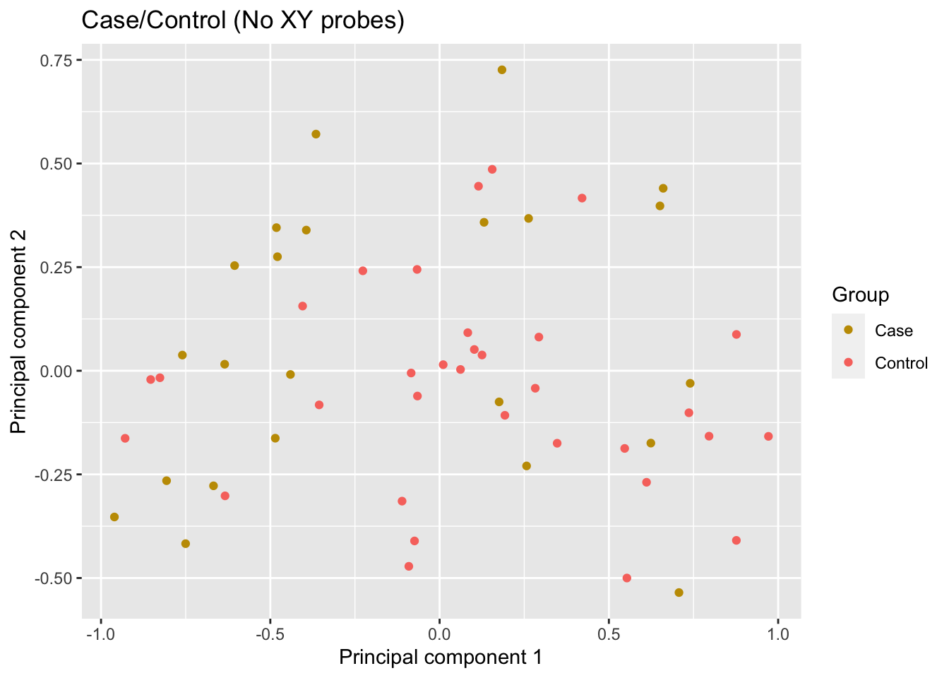
| Version | Author | Date |
|---|---|---|
| fb164d5 | JovMaksimovic | 2020-09-22 |
Estimate cell type proportions
Estimate the cell type proportions for the patient samples using the combined reference panel. As prevously determined, we are using the preprocessQuantile normalisation and have modified the estimateCellCounts2 function to only operate on the probes retained following quality control.
lavageRef <- rgSet[, cells]
colData(lavageRef)$CellType <- colData(lavageRef)$Sample_Group

patientSamps <- rgSet[, run]
sampleNames(patientSamps) <- info$Sample_source

props <- estimateCellCounts2(rgSet = patientSamps,
                                  compositeCellType = "Lavage",
                                  processMethod = "preprocessQuantile",
                                  probeSelect = "any",
                                  cellTypes = unique(targets$Sample_Group[cells]),
                                  referencePlatform =
                                    "IlluminaHumanMethylationEPIC",
                                  referenceset = "lavageRef",
                                  IDOLOptimizedCpGs = NULL,
                                  returnAll = TRUE,
                                  meanPlot = FALSE,
                                  keepProbes = rownames(mValsNoXY))
props$counts
EpithelialCell Macrophage Granulocyte Lymphocyte
M1C085b11 0.09477622 0.8472451 2.708448e-02 0.04023922
M1C074b10 0.12813101 0.7963481 3.867836e-02 0.05056298
M1C107b13 0.15978945 0.3016326 2.191895e-01 0.34509071
M1C086c11 0.03936756 0.9014079 5.780111e-03 0.05386626
M1C059c09 0.17976756 0.6241948 1.485435e-01 0.07067267
M1C108b13 0.05960772 0.8494110 5.000704e-02 0.04851297
P1C195b13 0.10542283 0.8320775 1.734723e-18 0.07005997
P1C171b11 0.37057997 0.6044666 4.594886e-02 0.02016715
P1C132b09 0.32543835 0.3383817 1.114962e-01 0.25088764
P1C139c09 0.05007595 0.6154065 2.650852e-01 0.09108060
P1C141b09 0.23141678 0.5751563 1.526022e-01 0.07264526
P1C174a11 0.55110012 0.3175145 3.941545e-02 0.13925846
P1C152b10 0.23909782 0.7050948 5.125415e-02 0.03256925
M1C077b10 0.09783183 0.6732710 1.479130e-01 0.09506376
M1C073b10 0.09591964 0.7381249 1.183965e-01 0.06372161
M1C081b10 0.16114732 0.2621753 4.069335e-01 0.20908039
M1C075b10 0.02909718 0.2547810 6.618983e-01 0.07091994
M1C079b10 0.28173934 0.2859430 1.766344e-01 0.27560116
M1C100b12 0.37711248 0.4850820 1.090802e-01 0.06853646
M1C122c14 0.29234803 0.5360451 1.388963e-02 0.15867791
P1C192b13 0.05421865 0.4678598 4.015643e-01 0.09819544
P1C167b11 0.15930226 0.6824067 2.185901e-02 0.14367306
P1C185b12 0.15739329 0.2056761 5.141837e-01 0.14234648
P1C165a10 0.07703830 0.8659905 2.384053e-02 0.03904757
P1C187b12 0.06228121 0.8020950 9.252901e-02 0.05404473
P1C166b11 0.12400205 0.1495986 6.899288e-01 0.06201218
P1C176b11 0.39139216 0.1979993 1.511386e-01 0.29320273
P1C182b12 0.36395744 0.4208833 0.000000e+00 0.20829986
M1C111b13 0.20322642 0.4254285 2.772779e-01 0.16461164
M1C123b14 0.05020962 0.8457585 7.481237e-02 0.03632896
M1C113b13 0.16966654 0.5748006 1.947762e-01 0.10451506
M1C125b14 0.31334014 0.4785268 1.113705e-01 0.12539296
M1C127b14 0.17374203 0.4608760 3.555295e-01 0.05521545
M1C109b13 0.27550559 0.4916701 1.627464e-01 0.11265965
M1C129b14 0.18591973 0.3431837 2.765491e-01 0.21766000
M1C117b14 0.07516300 0.3825491 3.921328e-01 0.16078446
P1C193b13 0.40835123 0.3659380 2.937709e-01 0.00000000
P1C178b11 0.18768672 0.7291993 4.805197e-03 0.08945491
P1C180b12 0.43856528 0.2345124 2.184903e-01 0.14168721
P1C213b14 0.17382311 0.5091199 2.750458e-01 0.07655560
P1C183b12 0.12773483 0.7259453 1.075547e-01 0.06492233
P1C170b11 0.35429957 0.4382421 1.833941e-01 0.06522500
P1C210b14 0.10414377 0.7563290 2.305462e-02 0.11867634
P1C161b10 0.15553470 0.4377452 4.034468e-01 0.03454761
P1C169b11 0.18991124 0.1780199 6.063379e-01 0.05642318
P1C163a09 0.20875538 0.5448154 2.315999e-02 0.22446091
P1C184b12 0.14085622 0.5566287 2.175659e-01 0.12661226
M1C126b14 0.43051469 0.4134157 7.660544e-02 0.11236232
P1C188b12 0.26391630 0.7057032 3.150925e-02 0.02776923
P1C224a14 0.14531520 0.2588730 5.589643e-01 0.07327991
P1C201b13 0.25622541 0.6356608 3.783866e-02 0.09368967
P1C140b09 0.04358499 0.7849878 1.147772e-01 0.06515646
P1C134b09 0.10999591 0.2224780 5.654328e-01 0.12585727
P1C156b10 0.16466150 0.5985766 5.584259e-02 0.19564627
P1C159b10 0.15102724 0.5418886 2.165660e-01 0.13803059
P1C136b09 0.13528982 0.4724800 2.471263e-01 0.16135221Explore the variation in the data
Principal components analysis
Principal components analysis (PCA) allows us to mathematically determine the sources of variation in the data. We can then investigate whether these correlate with any of the specifed covariates. First, we calculate the principal components. The scree plot belows shows us that most of the variation in this data is captured by the top 3-5 principal components.
PCs <- prcomp(t(mValsNoXY[, run]), center = TRUE,
              scale = TRUE, retx=TRUE)
loadings = PCs$x # pc loadings
plot(PCs, type="lines") # scree plot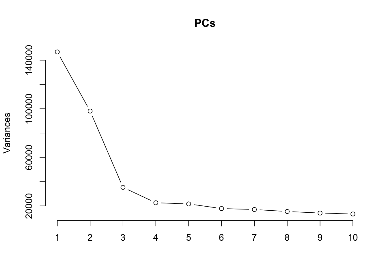
| Version | Author | Date |
|---|---|---|
| fb164d5 | JovMaksimovic | 2020-09-22 |
Collect all of the known sample traits.
nGenes = nrow(mValsNoXY)
nSamples = ncol(mValsNoXY[, run])
datTraits <- info %>% inner_join(rownames_to_column(data.frame(props$counts)),
                                 by = c("Sample_source" = "rowname")) %>%
  dplyr::select(-Sample_ID, -Sample_run, -Basename, -ID, -Pair, -Status,
                -Sample_source) %>%
  mutate_at("BAL_Age", as.numeric) %>%
  mutate(Sample_Group = as.numeric(factor(Sample_Group, labels = 1:2)),
         Sex = as.numeric(factor(Sex, labels = 1:2))) %>%
  mutate(BMI = replace(BMI, is.na(BMI), median(BMI, na.rm = TRUE)))

head(datTraits)
Sample_Group BAL_Age Sex BMI EpithelialCell Macrophage Granulocyte
1 2 1.36 2 15.220 0.09477622 0.8472451 0.027084481
2 1 1.00 2 17.375 0.12813101 0.7963481 0.038678355
3 2 1.49 1 17.375 0.15978945 0.3016326 0.219189543
4 1 1.16 2 16.090 0.03936756 0.9014079 0.005780111
5 2 1.44 2 17.375 0.17976756 0.6241948 0.148543537
6 1 1.19 2 17.330 0.05960772 0.8494110 0.050007039
Lymphocyte
1 0.04023922
2 0.05056298
3 0.34509071
4 0.05386626
5 0.07067267
6 0.04851297Correlate known sample traits with the top 20 principal components. This can help us determine which traits are potentially contributing to the main sources of variation in the data and should thus be included in our statistical analysis.
The correlation plot shows that differences in cell type proportions between samples are contributing to a lot of the variation in the top 3 principal components. However, case/control (Sample_Group), BMI, age and sex do not seem to be contributing to much of the variation in this data.
moduleTraitCor <- suppressWarnings(cor(loadings[, 1:20], datTraits, use = "p"))
moduleTraitPvalue <- WGCNA::corPvalueStudent(moduleTraitCor, (nSamples-2))
textMatrix <- paste(signif(moduleTraitCor, 2), "\n(",
signif(moduleTraitPvalue, 1), ")", sep = "")
dim(textMatrix) <- dim(moduleTraitCor)
## Display the correlation values within a heatmap plot
par(cex=0.75, mar = c(6, 8.5, 3, 3))
WGCNA::labeledHeatmap(Matrix = t(moduleTraitCor),
xLabels = colnames(loadings)[1:20],
yLabels = names(datTraits),
colorLabels = FALSE,
colors = WGCNA::blueWhiteRed(6),
textMatrix = t(textMatrix),
setStdMargins = FALSE,
cex.text = 0.5,
zlim = c(-1,1),
main = paste("PCA-trait relationships: Top 20 PCs"))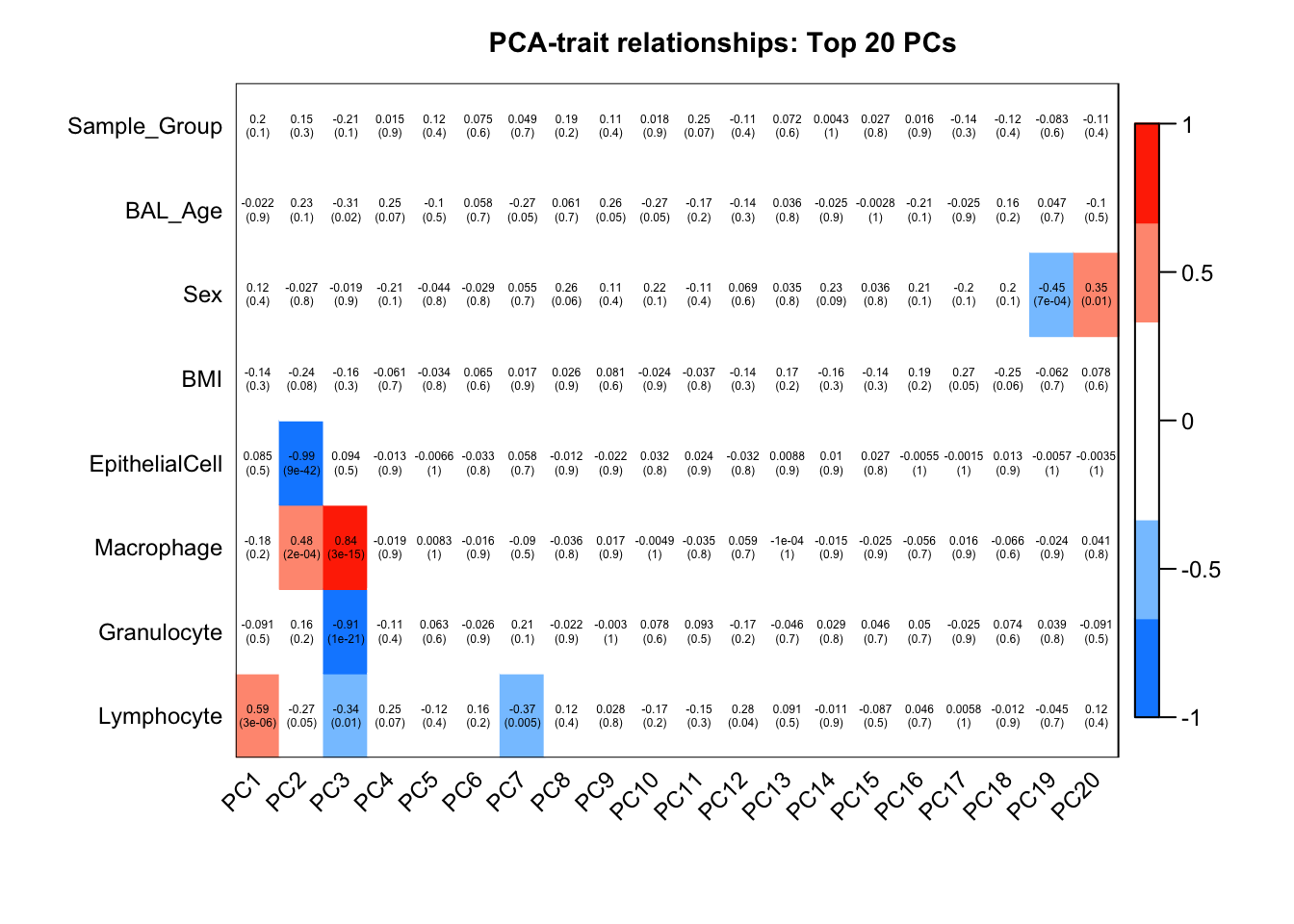
| Version | Author | Date |
|---|---|---|
| fb164d5 | JovMaksimovic | 2020-09-22 |
Visualise the variation
MDS plot coloured by estimated cell type proportions, stratified by cell type. As expected from the PCA-trait correlations, we can see a cell type proportion trend captured in the top 2 components, particularly driven by macrophages and granulocytes.
reshape2::melt(props$counts) %>%
  rename(sample = Var1, cell = Var2, prop = value) %>%
  inner_join(info, by = c("sample" = "Sample_source")) %>%
  dplyr::select(-Basename, -BAL_Age) -> dat

mds <- plotMDS(mValsNoXY[, run], top = 1000, gene.selection="common",
               plot = FALSE)
dat %>% inner_join(tibble(x = mds$x,
                          y = mds$y,
                          Sample_ID = names(mds$x))) -> mdat
Joining, by = "Sample_ID"p <- ggplot(mdat, aes(x = x, y = y, colour = prop)) +
geom_point(aes(shape = Sample_Group)) +
facet_wrap(vars(cell), ncol = 2, nrow = 2) +
labs(colour = "Est. Proportion",
shape = "Status",
x = "Principal component 1",
y = "Principal component 2") +
ggtitle("Case/control (No XY probes)") +
scale_colour_viridis_c(option = "magma")
p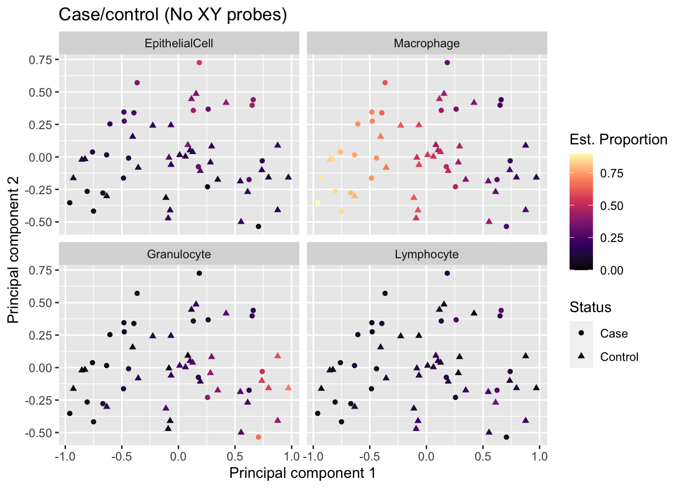
| Version | Author | Date |
|---|---|---|
| fb164d5 | JovMaksimovic | 2020-09-22 |
Standard differential methylation analysis
Comparison of cases versus controls using, taking into account estimated cell type proportions. No other variables are included as they do not appear to be contributing to much of the variation in this data.
CpG probe-wise linear models were fitted to determine differences in methylation between cases and controls using the limma package (Ritchie et al. 2015). Differentially methylated probes (DMPs) were identified using empirical Bayes moderated t-tests (Smyth 2005), performing robust empirical Bayes shrinkage of the gene-wise variances to protect against hypervariable probes (Phipson et al. 2016). P-values were adjusted for multiple testing using the Benjamini-Hochberg procedure (Benjamini and Hochberg 1995).
There are no statistically significant differences between cases and controls at FDR < 0.1.
cellEst <- data.frame(props$counts)
AEC <- cellEst$EpithelialCell
lymph <- cellEst$Lymphocyte
gran <- cellEst$Granulocyte
mac <- cellEst$Macrophage

design <- model.matrix.lm(~0 + Sample_Group + AEC + lymph + gran + mac ,
                       data = info)
colnames(design)[1:2] <- c("case", "control")

cont <- makeContrasts(caseVctrl = case - control,
                      levels = design)
fit <- lmFit(data, design)
cfit <- contrasts.fit(fit, cont)
fit2 <- eBayes(cfit, robust = TRUE)

summary(decideTests(fit2, p.value = 0.05))
caseVctrl
Down 0
NotSig 695764
Up 0These are the top 10 ranked CpGs.
data.frame(annEPIC) %>% dplyr::slice(match(rownames(fit2),
                                       rownames(annEPIC))) %>%
  dplyr::select(chr, pos, UCSC_RefGene_Name,
                UCSC_RefGene_Group) -> ann

top <- topTable(fit2, coef = "caseVctrl", genelist = ann, number = 100)
head(top, n = 10)
chr pos UCSC_RefGene_Name
cg19905587 chr2 85554135 TGOLN2
cg16284279 chr6 77743952
cg12145739 chr14 24912198 SDR39U1;SDR39U1;SDR39U1;SDR39U1;LOC101927045
cg12250896 chr10 134001112 DPYSL4
cg12041429 chr17 7585875 TP53;TP53;TP53;TP53
cg09850105 chr8 145111516 OPLAH
cg07506458 chr19 38899594 FAM98C
cg04477130 chr2 242986565 LINC01237
cg19283778 chr6 96917485
cg15556709 chr7 43739176 C7orf44
UCSC_RefGene_Group logFC AveExpr t
cg19905587 Body 0.3386682 -2.074180 5.408393
cg16284279 -0.5154492 1.339840 -5.339147
cg12145739 TSS200;TSS200;TSS200;TSS200;Body -0.4703872 -1.451730 -5.225031
cg12250896 Body 0.4903976 -3.618641 5.145187
cg12041429 5'UTR;5'UTR;5'UTR;5'UTR 0.3743635 2.992638 5.068122
cg09850105 Body 0.2387193 1.643058 5.039243
cg07506458 3'UTR 0.3379946 3.154448 5.002725
cg04477130 Body 0.3154275 2.422324 4.993917
cg19283778 -0.3340654 1.489536 -4.920944
cg15556709 5'UTR 0.4189949 2.641004 4.841584
P.Value adj.P.Val B
cg19905587 1.413404e-06 0.5479681 2.414257
cg16284279 1.820318e-06 0.5479681 2.267782
cg12145739 2.751755e-06 0.5479681 2.027958
cg12250896 3.668914e-06 0.5479681 1.860356
cg12041429 4.837135e-06 0.5479681 1.698801
cg09850105 5.349973e-06 0.5479681 1.640176
cg07506458 6.109915e-06 0.5479681 1.561909
cg04477130 6.300620e-06 0.5479681 1.543973
cg19283778 8.171824e-06 0.6317401 1.391037
cg15556709 1.081983e-05 0.6642332 1.225617These are the beta values of the top 12 ranked CpGs stratified by case/control status. Although there appears to be very small differences in the means of the two groups, the variability is too great to reach statistical significance.
bdat <- reshape2::melt(bValsNoXY[, run])
bdat$group <- rep(info$Sample_Group, each = nrow(bValsNoXY))

p <- vector("list", 12)

for(i in 1:length(p)){
p[[i]] <- ggplot(data = subset(bdat, bdat$Var1 == rownames(top)[i]),
       aes(x = group, y = value, colour = group)) +
  geom_jitter(width = 0.25) +
  stat_summary(fun = "mean", geom = "crossbar") +
  labs(x = "Status", y = "Beta value", colour = "Status") +
  ggtitle(rownames(top)[i], subtitle = top$UCSC_RefGene_Name[i]) +
  theme(plot.title = element_text(size = 8),
        plot.subtitle = element_text(size = 7),
        axis.title = element_text(size = 8),
        axis.text.x = element_text(size = 7))
}

(p[[1]] | p[[2]] | p[[3]]) /
  (p[[4]] | p[[5]] | p[[6]]) /
  (p[[7]] | p[[8]] | p[[9]]) /
  (p[[10]] | p[[11]] | p[[12]]) +
  plot_layout(guides = "collect") & theme(legend.position = "bottom")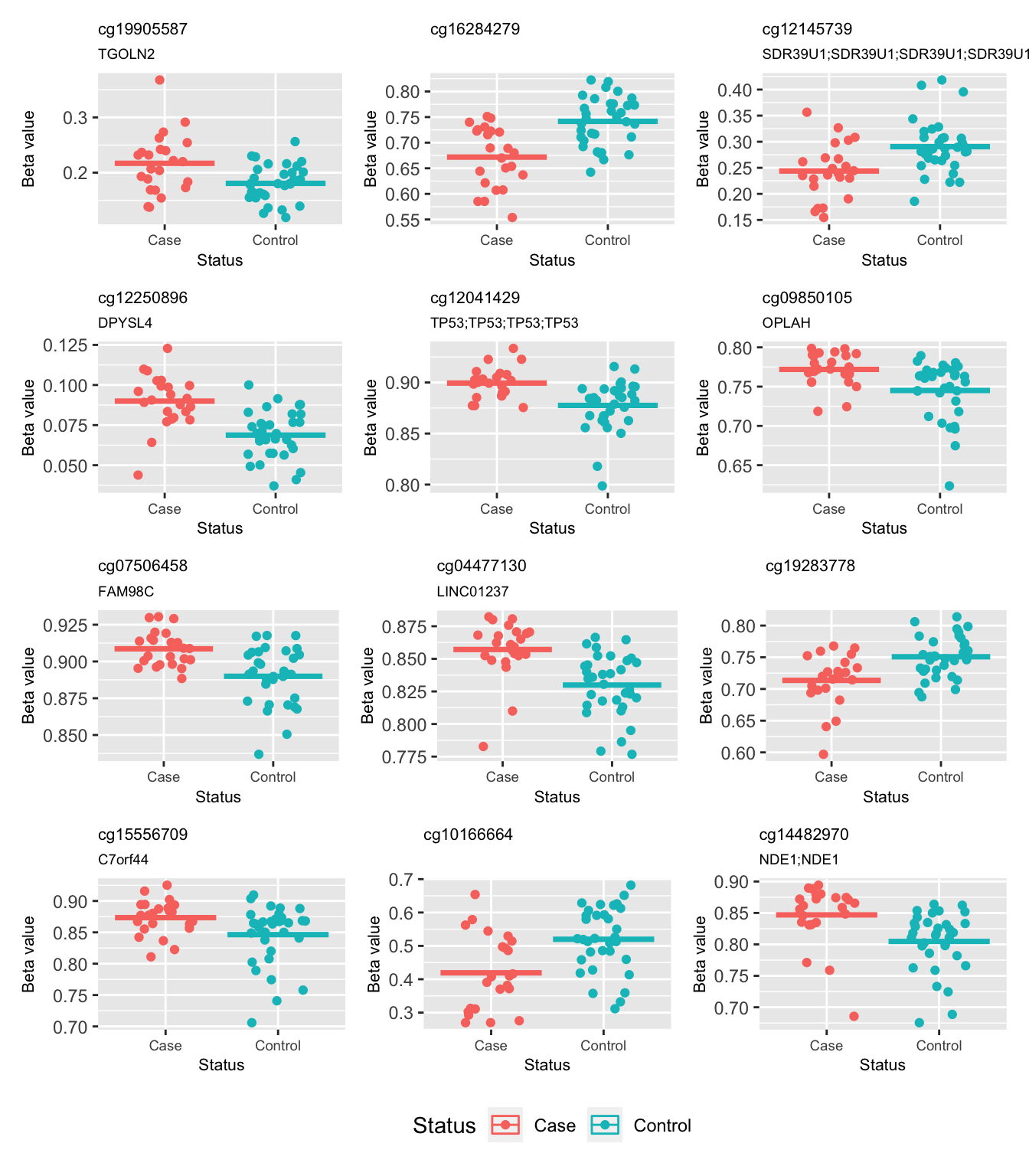
| Version | Author | Date |
|---|---|---|
| fb164d5 | JovMaksimovic | 2020-09-22 |
Write top 100 ranked CpGs to file.
write.csv(top, file = here("output/case-ctrl-oneyr.csv"))RUV Analysis
As recommended in Jaffe et al. (2014), adjust for cell type proportions using RUV. Identify cell type discriminating probes using the any option, which selects the 2 x 100 probes (with F-stat p-value < 1E-8) with the greatest magnitude of difference regardless of direction of effect.
mSetSqFlt$CellType <- as.character(targets$Sample_Group)

pAny <- minfi:::pickCompProbes(mSet = mSetSqFlt[rownames(data), cells],
                               probeSelect = "any",
                               numProbes = 100,
                               compositeCellType = "Lavage",
                               cellTypes = unique(targets$Sample_Group[cells]))
Use a heatmap to visulalise the methylation of the cell type discriminating probes in the cell sorted samples and the patient samples. As expected, the reference panel samples strongly cluster by cell type based using these probes. We can also see the variability in the patient samples at these loci, which we expect to be driven by differences in cell type proportions. The patient samples do not cluster by case/control status.
par(mfrow=c(2,1))
aheatmap(bValsNoXY[rownames(bValsNoXY) %in% rownames(pAny$coefEsts), cells],
         annCol = list(Cell_Types = as.character(targets$Sample_Group[cells])),
         labCol = NA, labRow = NA,
         main="Cell type discriminating probes (reference panel)")
aheatmap(data[rownames(data) %in% rownames(pAny$coefEsts), ],
         annCol = list(Group = as.character(info$Sample_Group)),
         labCol = NA, labRow = NA,
         main="Cell type discriminating probes (patient samples)")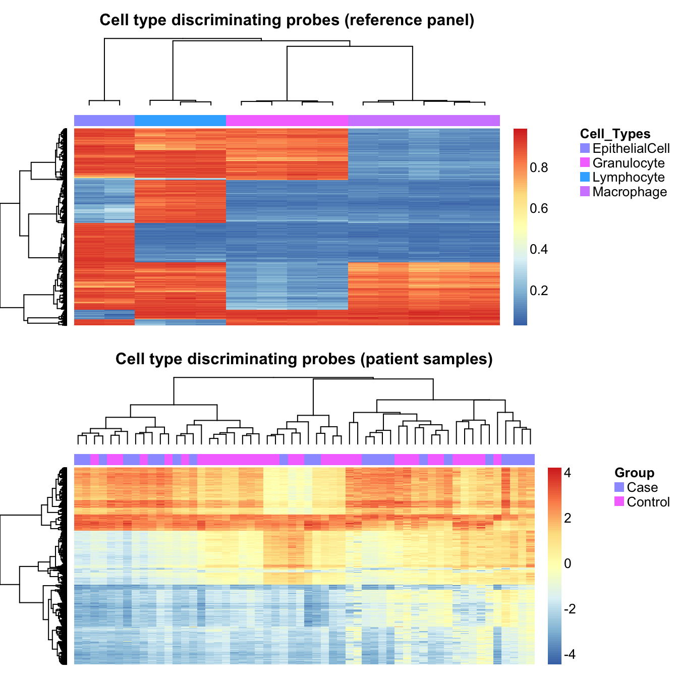
| Version | Author | Date |
|---|---|---|
| fb164d5 | JovMaksimovic | 2020-09-22 |
Explore the structure of the data using all probes and cell type discriminating (negative control) probes. As seen in previous analyses, there is no obvious clustering by case/control status or sex.
YA <- t(data)
ctl <- rownames(data) %in% rownames(pAny$coefEsts)

gg_additions <- list(aes(color = info$Sample_Group,
                         shape = info$Sex,
                         size = 5, alpha = .7),
                     labs(color = "Status", shape = "Sex"),
                     scale_size_identity(guide = "none"),
                     scale_alpha(guide = "none"),
                     theme(legend.text = element_text(size = 8),
                           legend.title = element_text(size = 10)),
                     guides(color = guide_legend(override.aes = list(size = 4)),
                            shape = guide_legend(override.aes = list(size = 4))))
p1 <- ruv::ruv_svdplot(YA) +
  gg_additions +
  theme(legend.position = "none") +
  ggtitle("All probes")
p2 <- ruv::ruv_svdplot(YA[, ctl]) +
  gg_additions +
  ggtitle("Negative control probes")
p1 | p2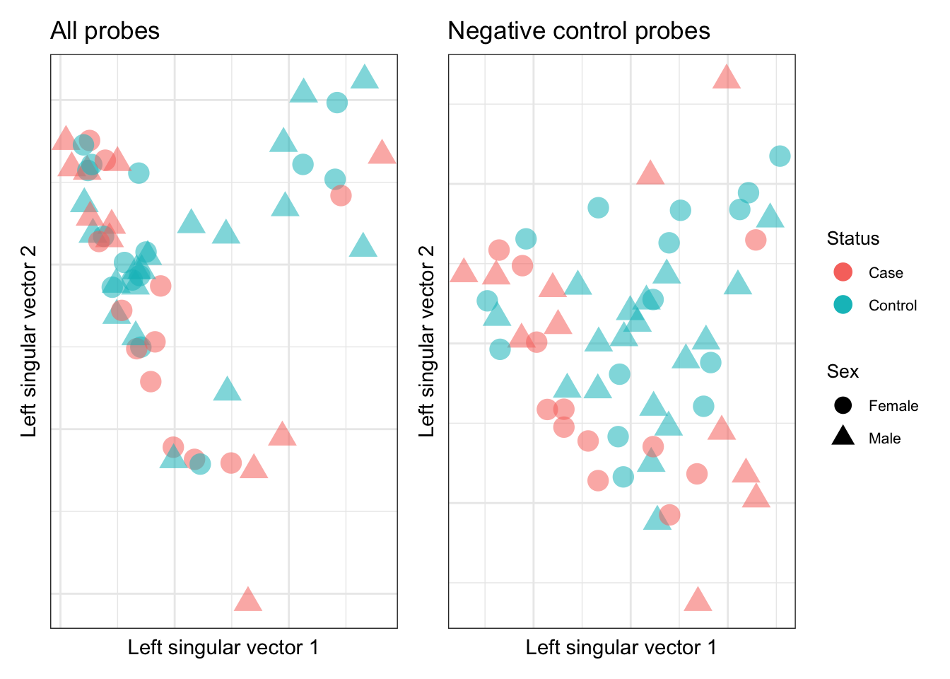
| Version | Author | Date |
|---|---|---|
| fb164d5 | JovMaksimovic | 2020-09-22 |
As previously objserved, the major effect is the difference in cell type proportions particularly for macrophages and granulocytes.
mds <- plotMDS(data, top = 1000, gene.selection="common",
               plot = FALSE)
dat %>% inner_join(tibble(x = mds$x,
                          y = mds$y,
                          Sample_ID = names(mds$x))) -> mdat
Joining, by = "Sample_ID"p <- ggplot(mdat, aes(x = x, y = y, colour = prop)) +
geom_point(aes(shape = Sample_Group)) +
facet_wrap(vars(cell), ncol = 2) +
labs(colour = "Status",
x = "Principal component 1",
y = "Principal component 2") +
ggtitle("Case/control (No XY probes)") +
scale_color_viridis_c(option = "magma")
p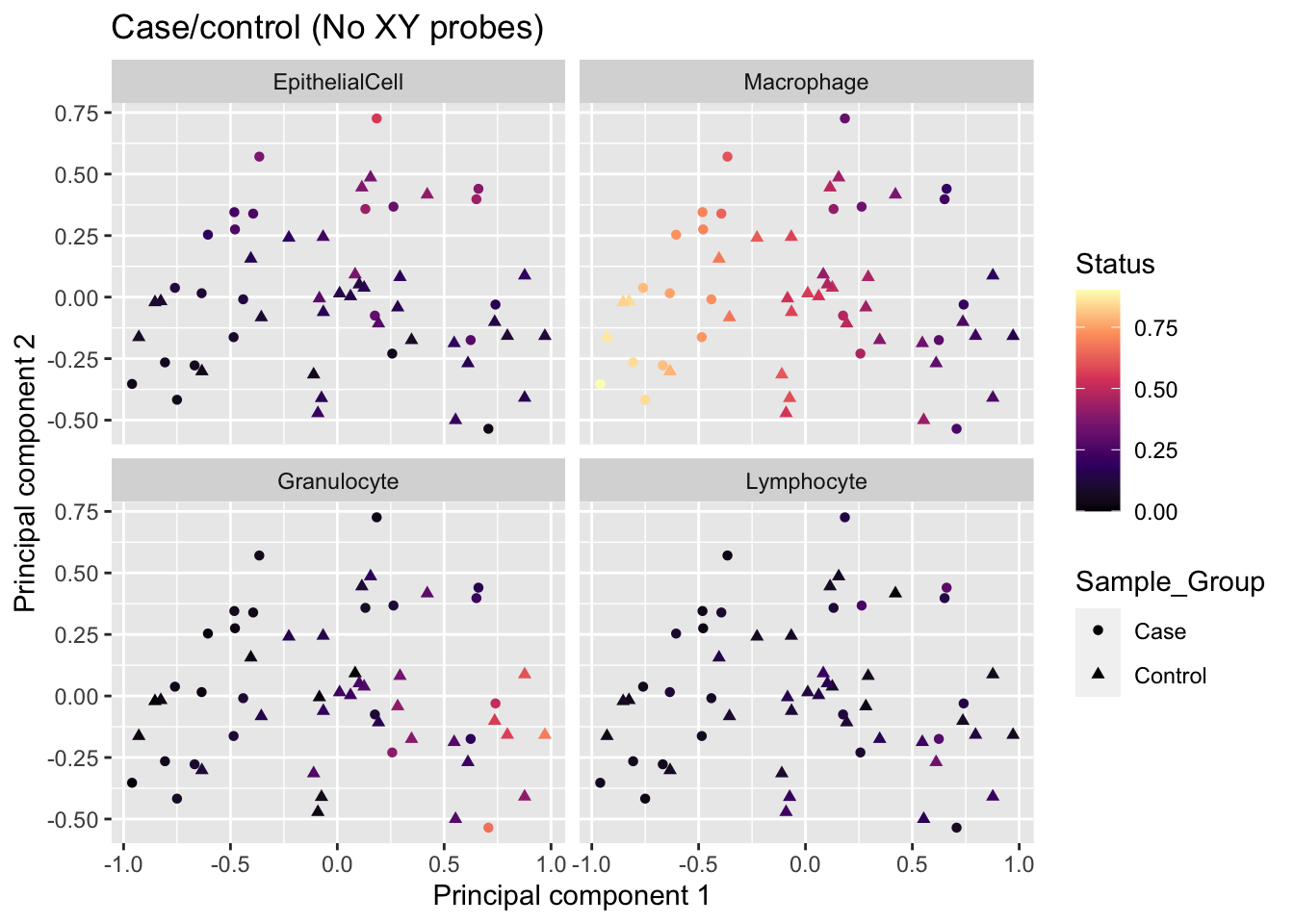
| Version | Author | Date |
|---|---|---|
| fb164d5 | JovMaksimovic | 2020-09-22 |
Use scree plots to examine how much of the variation is explained by the various components in the data. As shown in the PCA-trait analysis, the top 3 components capture the majority of the variation in the data and is driven by differences in cell type proportions. This can be observed for both all probes and in the negative control probes.
p1 <- ruv::ruv_scree(YA) +
  ggtitle("All probes")
p2 <- ruv::ruv_scree(YA[,ctl]) +
  ggtitle("Negative control probes")
p1 | p2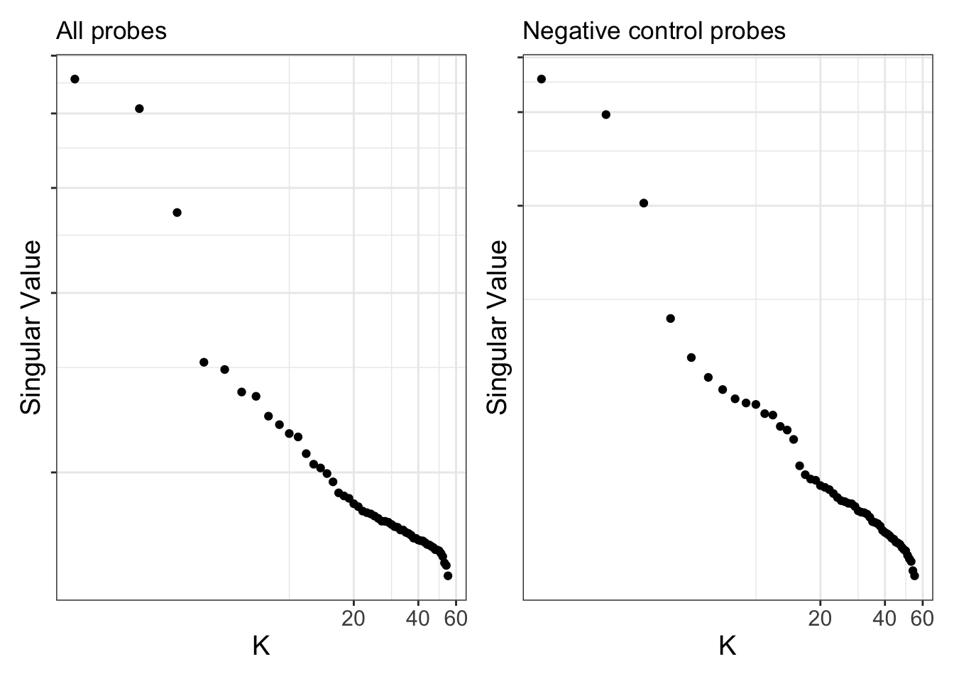
| Version | Author | Date |
|---|---|---|
| fb164d5 | JovMaksimovic | 2020-09-22 |
Unadjusted analysis
First run an unadjusted differential methylation analysis comparing cases and controls. There are no significant CpGs at FDR < 0.1.
caseCtrl <- factor(info$Sample_Group)

fitUnadj <- ruv::RUV4(YA, X = caseCtrl, ctl = ctl, k = 0)
fitUnadjSum <- ruv::ruv_summary(YA, fitUnadj, colinfo = ann)

table(fitUnadjSum$C$p.BH_X1.Control < 0.1)
 FALSE
695764
These are the beta values of the top 12 ranked CpGs stratified by case/control status for the unadjusted analysis. Again, we observe a small difference in means between the groups but the variability is too great to reach significance.
p <- vector("list", 12)

for(i in 1:length(p)){
p[[i]] <- ggplot(data = subset(bdat,
                               bdat$Var1 == rownames(fitUnadjSum$C)[i]),
       aes(x = group, y = value, colour = group)) +
  geom_jitter(width = 0.25) +
  stat_summary(fun = "mean", geom = "crossbar") +
  labs(x = "Status", y = "Beta value", colour = "Status") +
  ggtitle(rownames(fitUnadjSum$C)[i],
          subtitle = fitUnadjSum$C$UCSC_RefGene_Name[i]) +
  theme(plot.title = element_text(size = 8),
        plot.subtitle = element_text(size = 7),
        axis.title = element_text(size = 8),
        axis.text.x = element_text(size = 7))
}

(p[[1]] | p[[2]] | p[[3]]) /
  (p[[4]] | p[[5]] | p[[6]]) /
  (p[[7]] | p[[8]] | p[[9]]) /
  (p[[10]] | p[[11]] | p[[12]]) +
  plot_layout(guides = "collect") & theme(legend.position = "bottom")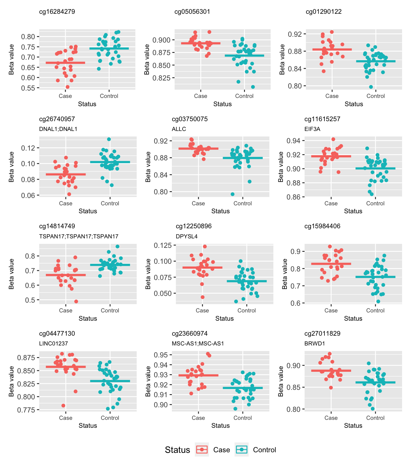
| Version | Author | Date |
|---|---|---|
| fb164d5 | JovMaksimovic | 2020-09-22 |
Adjusted analysis
Perform differential methylation analysis using RUV4 and designate the cell type discriminating as negative control probes to adjust for differences in cell type proportions. From our previous analyses, we know that the top 3 principal components capture most of the variation due to cell type proportion differences so set k=3.
There are 7 significantly differentially methylated CpGs at FDR < 0.1.
fitAdj <- RUVfit(data, X = caseCtrl, ctl = ctl, k = 3, method = "ruv4")
fitAdjSum <- RUVadj(data, fitAdj, cpginfo = ann)

table(fitAdjSum$C$p.BH_X1.Control < 0.1)
 FALSE   TRUE
695757      7
Use p-value histograms to check that the adjustment is improving our analysis. A good p-value distribution has a peak for low values and a uniform distribution for the larger values. The p-value distribution for the adjusted analysis shows an improvement over the unadjusted analysis.
p1 <- ruv::ruv_hist(fitUnadjSum) + ggtitle("Unadjusted analysis")
p2 <- ruv::ruv_hist(fitAdjSum) + ggtitle("Adjusted analysis (k=3)")
p1 | p2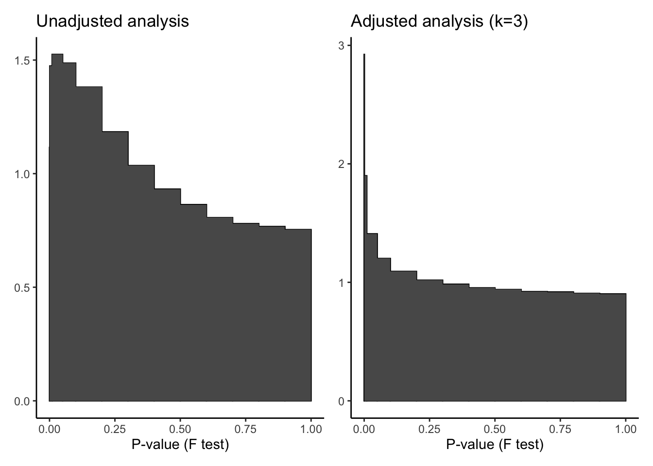
| Version | Author | Date |
|---|---|---|
| fb164d5 | JovMaksimovic | 2020-09-22 |
An MDS plot of the adjusted data no longer shows a cell type proportion trend in the top 2 principal componets.
Madj <- getAdj(Y = data, fit = fitAdj)
mds <- plotMDS(Madj, top = 1000, gene.selection="common",
               plot = FALSE)
dat %>% inner_join(tibble(x = mds$x,
                          y = mds$y,
                          Sample_ID = names(mds$x))) -> mdat
Joining, by = "Sample_ID"p <- ggplot(mdat, aes(x = x, y = y, colour = prop)) +
geom_point(aes(shape = Sample_Group)) +
facet_wrap(vars(cell), ncol = 2) +
labs(colour = "Status",
x = "Principal component 1",
y = "Principal component 2") +
ggtitle("Case/control (k = 3)") +
scale_color_viridis_c(option = "magma")
p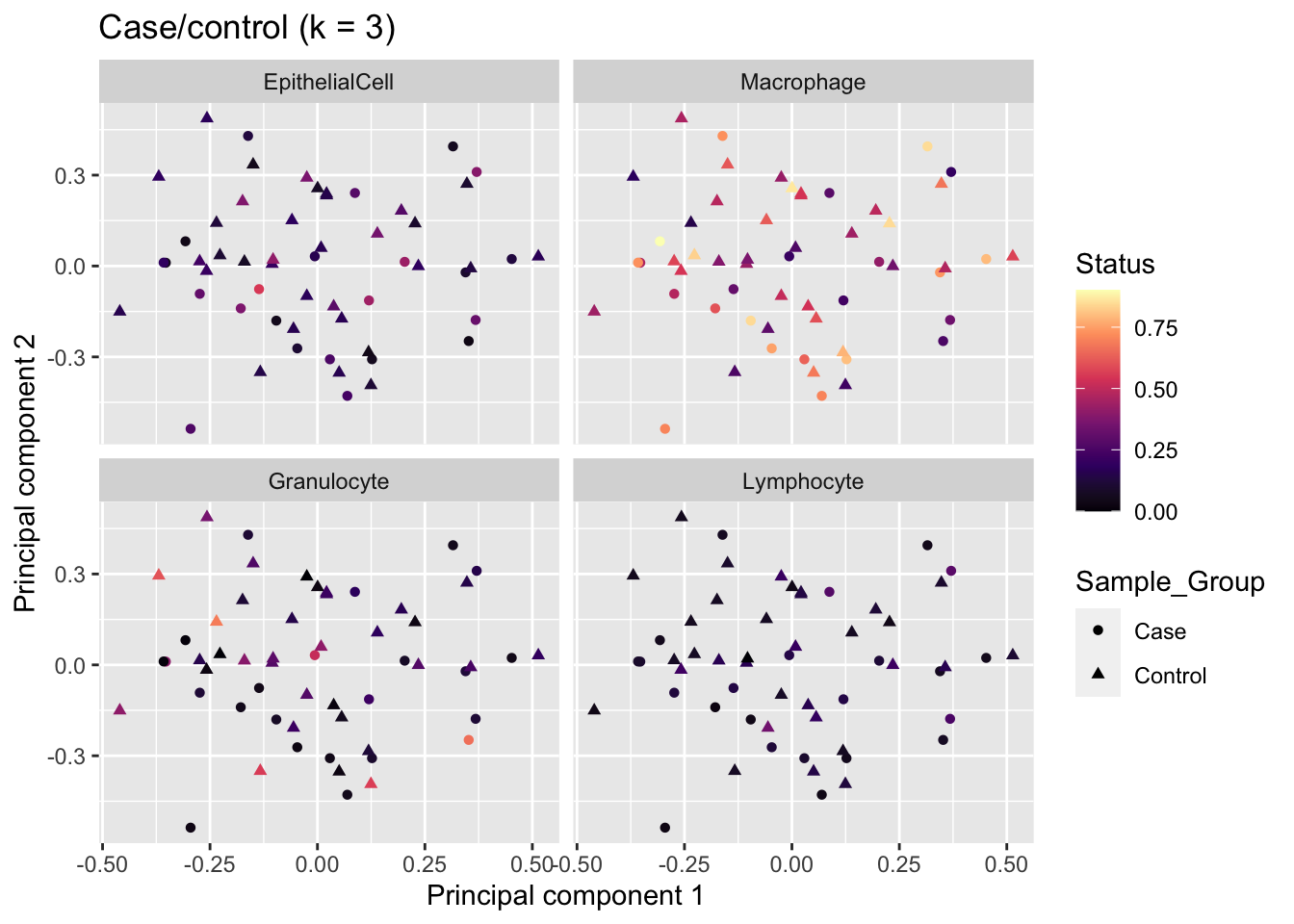
| Version | Author | Date |
|---|---|---|
| fb164d5 | JovMaksimovic | 2020-09-22 |
The top 10 ranked CpGs from the adjusted analysis.
               F.p     F.p.BH p_X1.Control p.BH_X1.Control b_X1.Control
CpG1  4.600305e-08 0.03200727 4.600305e-08      0.03200727   -0.2736275
CpG2  1.852958e-07 0.06446107 1.852958e-07      0.06446107    0.2095824
CpG3  4.964166e-07 0.08423628 4.964166e-07      0.08423628    0.3554793
CpG4  6.378621e-07 0.08423628 6.378621e-07      0.08423628    0.2546832
CpG5  6.727708e-07 0.08423628 6.727708e-07      0.08423628    0.4997063
CpG6  7.264211e-07 0.08423628 7.264211e-07      0.08423628    0.2134768
CpG7  9.687900e-07 0.09629274 9.687900e-07      0.09629274    0.2868584
CpG8  1.460669e-06 0.12427848 1.460669e-06      0.12427848    0.3190960
CpG9  1.926622e-06 0.12427848 1.926622e-06      0.12427848    0.1942865
CpG10 1.937024e-06 0.12427848 1.937024e-06      0.12427848   -0.3294484
          sigma2 var.b_X1.Control fit.ctl      mean
CpG1  0.02308838      0.001875536   FALSE  2.422324
CpG2  0.01528668      0.001241782   FALSE -2.896356
CpG3  0.04816956      0.003912954   FALSE -2.537235
CpG4  0.02532563      0.002057275   FALSE -1.812852
CpG5  0.09799925      0.007960765   FALSE  1.339840
CpG6  0.01801867      0.001463709   FALSE -3.004684
CpG7  0.03346614      0.002718552   FALSE -3.234123
CpG8  0.04314813      0.003505049   FALSE  1.489536
CpG9  0.01645530      0.001336712   FALSE  1.195571
CpG10 0.04734092      0.003845641   FALSE -2.074180
                                                              UCSC_RefGene_Group
CpG1                                                                        Body
CpG2                                                          TSS200;Body;TSS200
CpG3
CpG4                                                      TSS1500;Body;Body;Body
CpG5
CpG6
CpG7                                                         Body;Body;Body;Body
CpG8
CpG9  Body;Body;Body;Body;Body;Body;Body;Body;Body;Body;Body;Body;Body;Body;Body
CpG10                                                                       Body
These are the beta values of the top 12 ranked CpGs stratified by case/control status for the adjusted analysis. The faded points and the dotted line indicate the original data and its mean; the solid points and solid line represent the adjusted data and its mean. As expected, the variability has decraesed in the adjusted data.
ajdat <- reshape2::melt(ilogit2(Madj))
ajdat$group <- rep(info$Sample_Group, each = nrow(Madj))

p <- vector("list", 12)

for(i in 1:length(p)){
p[[i]] <- ggplot(data = subset(bdat, bdat$Var1 == rownames(fitAdjSum$C)[i]),
       aes(x = group, y = value, colour = group)) +
  geom_jitter(width = 0.25, alpha = 0.3) +
  stat_summary(fun = "mean", geom = "crossbar", linetype = "dotted",
               size = 0.25) +
  geom_jitter(data = subset(ajdat, ajdat$Var1 == rownames(fitAdjSum$C)[i]),
       aes(x = group, y = value, colour = group), width = 0.25) +
  stat_summary(data = subset(ajdat, ajdat$Var1 == rownames(fitAdjSum$C)[i]),
       aes(x = group, y = value, colour = group),
       fun = "mean", geom = "crossbar", size = 0.25) +
  labs(x = "Status", y = "Beta value", colour = "Status") +
  #ggtitle(rownames(fitAdjSum$C)[i], subtitle = fitAdjSum$C$UCSC_RefGene_Name[i]) +
  ggtitle(glue::glue("CpG{i}"))
  theme(plot.title = element_text(size = 8),
        plot.subtitle = element_text(size = 7),
        axis.title = element_text(size = 8),
        axis.text.x = element_text(size = 7))
}

(p[[1]] | p[[2]] | p[[3]]) /
  (p[[4]] | p[[5]] | p[[6]]) /
  (p[[7]] | p[[8]] | p[[9]]) /
  (p[[10]] | p[[11]]  | p[[12]] ) +
  plot_layout(guides = "collect") &
  theme(legend.position = "bottom")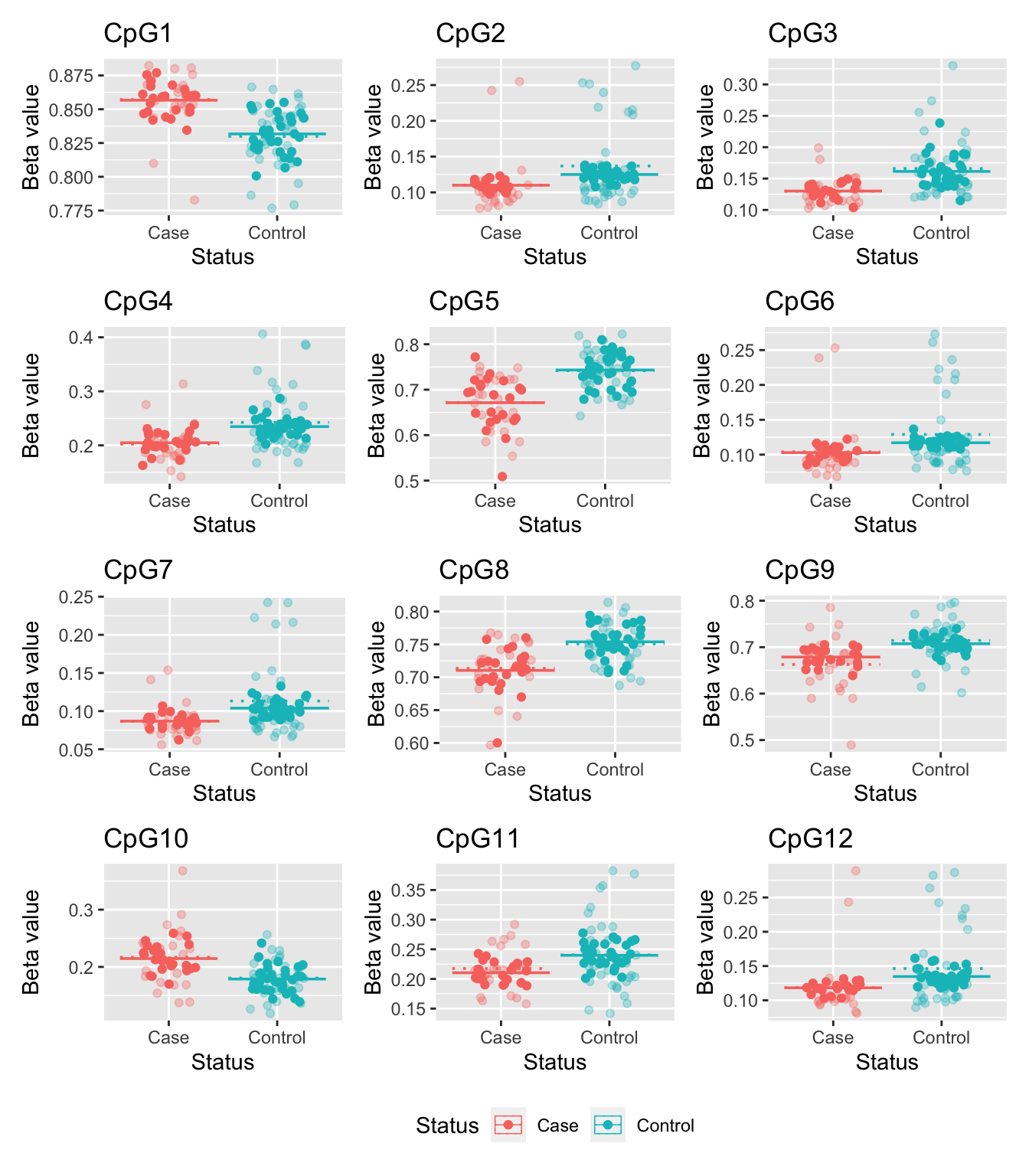
| Version | Author | Date |
|---|---|---|
| fb164d5 | JovMaksimovic | 2020-09-22 |
Write the top 100 ranked CpGs to a file.
write.csv(fitAdjSum$C[1:100,], file = here("output/case-ctrl-oneyr-ruv.csv"))Write adjusted beta values for significant probes to a file.
Write adjusted beta values for significant probes to a file, along with CpGs 10kb upstream and downstream of each significant CpG.
sessionInfo()R version 4.0.3 (2020-10-10)
Platform: x86_64-apple-darwin17.0 (64-bit)
Running under: macOS Mojave 10.14.6
Matrix products: default
BLAS: /Library/Frameworks/R.framework/Versions/4.0/Resources/lib/libRblas.dylib
LAPACK: /Library/Frameworks/R.framework/Versions/4.0/Resources/lib/libRlapack.dylib
locale:
[1] en_AU.UTF-8/en_AU.UTF-8/en_AU.UTF-8/C/en_AU.UTF-8/en_AU.UTF-8
attached base packages:
[1] stats4 parallel stats graphics grDevices utils datasets
[8] methods base
other attached packages:
[1] RColorBrewer_1.1-2
[2] NMF_0.23.0
[3] cluster_2.1.0
[4] rngtools_1.5
[5] pkgmaker_0.32.2
[6] registry_0.5-1
[7] BiocParallel_1.24.1
[8] patchwork_1.1.1
[9] forcats_0.5.0
[10] stringr_1.4.0
[11] dplyr_1.0.2
[12] purrr_0.3.4
[13] readr_1.4.0
[14] tidyr_1.1.2
[15] tibble_3.0.4
[16] tidyverse_1.3.0
[17] ggplot2_3.3.2
[18] FlowSorted.Blood.EPIC_1.8.0
[19] ExperimentHub_1.16.0
[20] AnnotationHub_2.22.0
[21] BiocFileCache_1.14.0
[22] dbplyr_2.0.0
[23] nlme_3.1-151
[24] quadprog_1.5-8
[25] genefilter_1.72.0
[26] IlluminaHumanMethylationEPICmanifest_0.3.0
[27] missMethyl_1.24.0
[28] IlluminaHumanMethylationEPICanno.ilm10b4.hg19_0.6.0
[29] IlluminaHumanMethylation450kanno.ilmn12.hg19_0.6.0
[30] minfi_1.36.0
[31] bumphunter_1.32.0
[32] locfit_1.5-9.4
[33] iterators_1.0.13
[34] foreach_1.5.1
[35] Biostrings_2.58.0
[36] XVector_0.30.0
[37] SummarizedExperiment_1.20.0
[38] Biobase_2.50.0
[39] MatrixGenerics_1.2.0
[40] matrixStats_0.57.0
[41] GenomicRanges_1.42.0
[42] GenomeInfoDb_1.26.2
[43] IRanges_2.24.1
[44] S4Vectors_0.28.1
[45] BiocGenerics_0.36.0
[46] limma_3.46.0
[47] here_1.0.1
[48] workflowr_1.6.2
loaded via a namespace (and not attached):
[1] tidyselect_1.1.0 htmlwidgets_1.5.3
[3] RSQLite_2.2.1 AnnotationDbi_1.52.0
[5] grid_4.0.3 munsell_0.5.0
[7] codetools_0.2-18 preprocessCore_1.52.0
[9] statmod_1.4.35 withr_2.3.0
[11] colorspace_2.0-0 knitr_1.30
[13] rstudioapi_0.13 labeling_0.4.2
[15] git2r_0.27.1 GenomeInfoDbData_1.2.4
[17] bit64_4.0.5 farver_2.0.3
[19] rhdf5_2.34.0 rprojroot_2.0.2
[21] vctrs_0.3.6 generics_0.1.0
[23] xfun_0.19 fastcluster_1.1.25
[25] R6_2.5.0 doParallel_1.0.16
[27] illuminaio_0.32.0 bitops_1.0-6
[29] rhdf5filters_1.2.0 reshape_0.8.8
[31] DelayedArray_0.16.0 assertthat_0.2.1
[33] promises_1.1.1 scales_1.1.1
[35] nnet_7.3-14 gtable_0.3.0
[37] WGCNA_1.69 rlang_0.4.9
[39] splines_4.0.3 rtracklayer_1.50.0
[41] impute_1.64.0 GEOquery_2.58.0
[43] checkmate_2.0.0 broom_0.7.3
[45] BiocManager_1.30.10 yaml_2.2.1
[47] reshape2_1.4.4 modelr_0.1.8
[49] GenomicFeatures_1.42.1 backports_1.2.1
[51] httpuv_1.5.4 Hmisc_4.4-2
[53] tools_4.0.3 gridBase_0.4-7
[55] nor1mix_1.3-0 ellipsis_0.3.1
[57] siggenes_1.64.0 dynamicTreeCut_1.63-1
[59] Rcpp_1.0.5 plyr_1.8.6
[61] base64enc_0.1-3 sparseMatrixStats_1.2.0
[63] progress_1.2.2 zlibbioc_1.36.0
[65] RCurl_1.98-1.2 prettyunits_1.1.1
[67] rpart_4.1-15 openssl_1.4.3
[69] haven_2.3.1 fs_1.5.0
[71] magrittr_2.0.1 data.table_1.13.4
[73] reprex_0.3.0 whisker_0.4
[75] hms_0.5.3 mime_0.9
[77] evaluate_0.14 xtable_1.8-4
[79] XML_3.99-0.5 jpeg_0.1-8.1
[81] mclust_5.4.7 readxl_1.3.1
[83] gridExtra_2.3 compiler_4.0.3
[85] biomaRt_2.46.0 crayon_1.3.4
[87] htmltools_0.5.0 later_1.1.0.1
[89] Formula_1.2-4 lubridate_1.7.9.2
[91] DBI_1.1.0 MASS_7.3-53
[93] rappdirs_0.3.1 Matrix_1.2-18
[95] cli_2.2.0 pkgconfig_2.0.3
[97] GenomicAlignments_1.26.0 foreign_0.8-80
[99] xml2_1.3.2 annotate_1.68.0
[101] ruv_0.9.7.1 multtest_2.46.0
[103] beanplot_1.2 rvest_0.3.6
[105] doRNG_1.8.2 scrime_1.3.5
[107] digest_0.6.27 rmarkdown_2.6
[109] base64_2.0 cellranger_1.1.0
[111] htmlTable_2.1.0 DelayedMatrixStats_1.12.1
[113] curl_4.3 shiny_1.5.0
[115] Rsamtools_2.6.0 lifecycle_0.2.0
[117] jsonlite_1.7.2 Rhdf5lib_1.12.0
[119] viridisLite_0.3.0 askpass_1.1
[121] fansi_0.4.1 pillar_1.4.7
[123] lattice_0.20-41 GO.db_3.12.1
[125] fastmap_1.0.1 httr_1.4.2
[127] survival_3.2-7 interactiveDisplayBase_1.28.0
[129] glue_1.4.2 png_0.1-7
[131] BiocVersion_3.12.0 bit_4.0.4
[133] stringi_1.5.3 HDF5Array_1.18.0
[135] blob_1.2.1 org.Hs.eg.db_3.12.0
[137] latticeExtra_0.6-29 memoise_1.1.0