Differential methylation analysis
Jovana Maksimovic
12/17/2018
Last updated: 2020-12-18
Checks: 7 0
Knit directory: paed-cf-methylation/
This reproducible R Markdown analysis was created with workflowr (version 1.6.2). The Checks tab describes the reproducibility checks that were applied when the results were created. The Past versions tab lists the development history.
Great! Since the R Markdown file has been committed to the Git repository, you know the exact version of the code that produced these results.
Great job! The global environment was empty. Objects defined in the global environment can affect the analysis in your R Markdown file in unknown ways. For reproduciblity it's best to always run the code in an empty environment.
The command set.seed(20200224) was run prior to running the code in the R Markdown file. Setting a seed ensures that any results that rely on randomness, e.g. subsampling or permutations, are reproducible.
Great job! Recording the operating system, R version, and package versions is critical for reproducibility.
Nice! There were no cached chunks for this analysis, so you can be confident that you successfully produced the results during this run.
Great job! Using relative paths to the files within your workflowr project makes it easier to run your code on other machines.
Great! You are using Git for version control. Tracking code development and connecting the code version to the results is critical for reproducibility.
The results in this page were generated with repository version a54eaf6. See the Past versions tab to see a history of the changes made to the R Markdown and HTML files.
Note that you need to be careful to ensure that all relevant files for the analysis have been committed to Git prior to generating the results (you can use wflow_publish or wflow_git_commit). workflowr only checks the R Markdown file, but you know if there are other scripts or data files that it depends on. Below is the status of the Git repository when the results were generated:
Ignored files:
    Ignored:    .DS_Store
    Ignored:    .Rhistory
    Ignored:    .Rproj.user/
    Ignored:    code/DNAm-based-age-predictor/
    Ignored:    data/.DS_Store
    Ignored:    data/1-year-old-cohort-with-data.csv
    Ignored:    data/9-year-old-cohort-as-pairs-with-data.csv
    Ignored:    data/9-year-old-cohort-as-pairs.xlsx
    Ignored:    data/BMI-Data.csv
    Ignored:    data/BMI-Data.xlsx
    Ignored:    data/CFGeneModifiers.csv
    Ignored:    data/Flow-Data-for-Reference-Panel-Original copy.csv
    Ignored:    data/Flow-Data-for-Reference-Panel-Original.csv
    Ignored:    data/Flow-Data-for-Reference-Panel-Scaled copy.csv
    Ignored:    data/Flow-Data-for-Reference-Panel-Scaled.csv
    Ignored:    data/Flow-Data-for-Reference-Panel.xls
    Ignored:    data/Horvath-27k-probes.csv
    Ignored:    data/Horvath-coefficients.csv
    Ignored:    data/Horvath-methylation-data.csv
    Ignored:    data/Horvath-mini-annotation.csv
    Ignored:    data/Horvath-sample-data.csv
    Ignored:    data/ageFile-final.txt
    Ignored:    data/arsq.rds
    Ignored:    data/idat-new/
    Ignored:    data/idat/
    Ignored:    data/loglrt.rds
    Ignored:    data/processedData.RData
    Ignored:    data/processedDataNew-old.RData
    Ignored:    data/processedDataNew.RData
    Ignored:    data/rawPatientBetas.rds
    Ignored:    data/~$9-year-old-cohort-as-pairs.xlsx
    Ignored:    output/Horvath-output.csv
    Ignored:    output/Horvath-output2.csv
    Ignored:    output/age.pred
    Ignored:    output/case-ctrl-oneyr-ruv-sig-adj-betas-expanded.csv
    Ignored:    output/case-ctrl-oneyr-ruv-sig-adj-betas.csv
    Ignored:    output/case-ctrl-oneyr-ruv.csv
    Ignored:    output/case-ctrl-oneyr.csv
    Ignored:    output/case-ctrl-paired.csv
    Ignored:    output/stderr.txt
    Ignored:    output/stdout.txt

Untracked files:
    Untracked:  MethylResolver.txt
    Untracked:  code/test.R

Unstaged changes:
    Modified:   analysis/ruvAnalysis.Rmd
Note that any generated files, e.g. HTML, png, CSS, etc., are not included in this status report because it is ok for generated content to have uncommitted changes.
These are the previous versions of the repository in which changes were made to the R Markdown (analysis/pairedAnalysis.Rmd) and HTML (docs/pairedAnalysis.html) files. If you've configured a remote Git repository (see ?wflow_git_remote), click on the hyperlinks in the table below to view the files as they were in that past version.
| File | Version | Author | Date | Message |
|---|---|---|---|---|
| Rmd | a54eaf6 | JovMaksimovic | 2020-12-18 | wflow_publish(c("analysis/dataExploreNew.Rmd", "analysis/estCellPropNew.Rmd", |
| html | 9e7a472 | JovMaksimovic | 2020-09-25 | Build site. |
| Rmd | bf55ba4 | JovMaksimovic | 2020-09-25 | wflow_publish("analysis/pairedAnalysis.Rmd") |
| html | 2d78700 | JovMaksimovic | 2020-09-18 | Build site. |
| Rmd | 4eae19b | JovMaksimovic | 2020-09-18 | wflow_publish(c("analysis/index.Rmd", "analysis/dataExploreNew.Rmd", |
Differential methylation analysis of 9 year old cohort
Load packages necessary for analysis.
library(here)
library(workflowr)
#Load Packages Required for Analysis
library(limma)
library(minfi)
library(missMethyl)
library(matrixStats)
library(IlluminaHumanMethylationEPICanno.ilm10b4.hg19)
library(IlluminaHumanMethylationEPICmanifest)
library(FlowSorted.Blood.EPIC)
library(ggplot2)
library(tidyverse)
library(patchwork)
library(BiocParallel)
source(here("code/functions.R"))
Load processed data
Load raw and processed data objects generated by exploratory analysis.
load(here("data/processedDataNew.RData"))
source(here("code/functions.R"))
Extract only the samples from the first cohort.
runOne <- targets$Sample_run %in% "Old" & !is.na(targets$Pair)
data <- mVals[, runOne]
info <- targets[runOne, ]
The multi-dimensional scaling (MDS) plot shows some weak clustering of the samples, although it does not appear to be purely driven by case/control status.
mds <- plotMDS(mValsNoXY[, runOne], top = 1000, gene.selection="common",
               plot = FALSE)
dat <- tibble(x = mds$x,
              y = mds$y,
              group = info$Sample_Group,
              pair = info$Pair)

p <- ggplot(dat, aes(x = x, y = y, label = pair)) +
  geom_text(aes(colour = group)) +
  labs(colour = "Group",
       x = "Principal component 1",
       y = "Principal component 2") +
  ggtitle("Pairs (No XY probes)") +
  scale_color_manual(values = pal)
p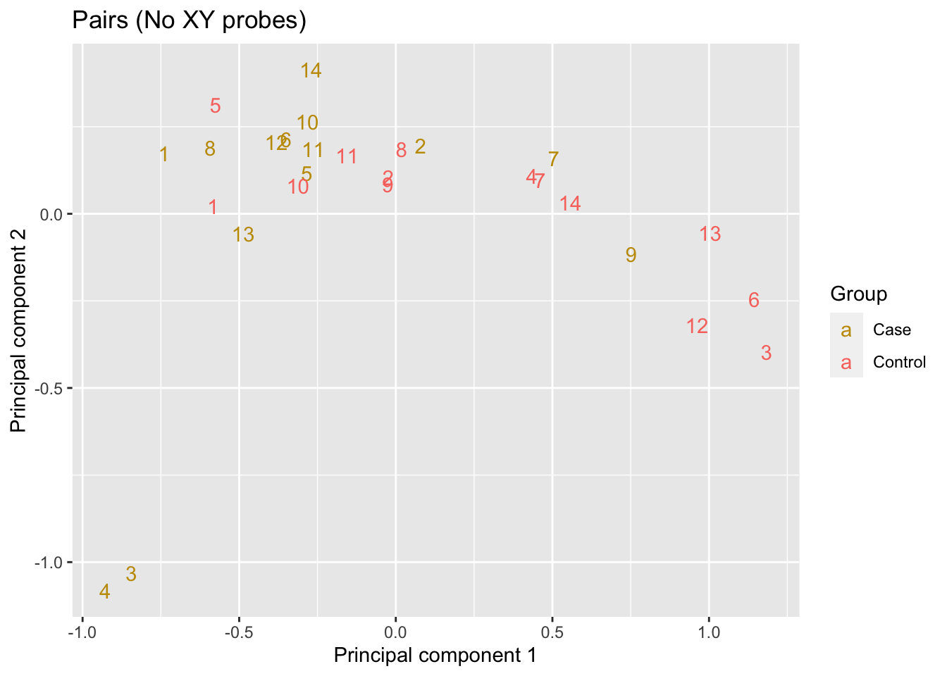
| Version | Author | Date |
|---|---|---|
| 2d78700 | JovMaksimovic | 2020-09-18 |
Estimate cell type proportions
Estimate the cell type proportions for the patient samples using the combined reference panel. As prevously determined, we are using the preprocessQuantile normalisation and have modified the estimateCellCounts2 function to only operate on the probes retained following quality control.
lavageRef <- rgSet[, cells]
colData(lavageRef)$CellType <- colData(lavageRef)$Sample_Group

patientSamps <- rgSet[, runOne]
sampleNames(patientSamps) <- info$Sample_source

props <- estimateCellCounts2(rgSet = patientSamps,
                                  compositeCellType = "Lavage",
                                  processMethod = "preprocessQuantile",
                                  probeSelect = "any",
                                  cellTypes = unique(targets$Sample_Group[cells]),
                                  referencePlatform =
                                    "IlluminaHumanMethylationEPIC",
                                  referenceset = "lavageRef",
                                  IDOLOptimizedCpGs = NULL,
                                  returnAll = TRUE,
                                  meanPlot = FALSE,
                                  keepProbes = rownames(mValsNoXY))
props$counts
EpithelialCell Macrophage Granulocyte Lymphocyte
57G 0.02928789 0.73796930 0.1299190 0.11795500
37H 0.02711103 0.65580637 0.2643458 0.06935392
23E12 0.11624431 0.39461442 0.4045330 0.13159166
08F 0.11132203 0.40227548 0.3832535 0.14163820
54F12 0.07693852 0.66316545 0.1845067 0.09487492
89C 0.06904478 0.00000000 0.8483914 0.08952296
55F12 0.01910191 0.72993159 0.2010050 0.06468691
32G 0.03809794 0.24003463 0.6528311 0.08298594
06F 0.16796010 0.44743066 0.2642869 0.15522540
14G 0.09635829 0.64769697 0.2317197 0.04548568
12F11 0.20109652 0.51619081 0.2074292 0.12280283
50G 0.05088999 0.03100595 0.9072657 0.01967462
52H 0.07464015 0.15160299 0.4006382 0.39085711
62H 0.13301180 0.20230927 0.4985003 0.19668390
26G 0.21711982 0.60259356 0.1644432 0.05312081
61G 0.03101789 0.40191348 0.4481375 0.15000627
53F 0.03807166 0.11996562 0.6939040 0.16940482
41G 0.05623525 0.37529692 0.4238317 0.16385327
48i 0.11718853 0.53680882 0.3071683 0.07380191
25G12 0.08057696 0.54910144 0.3207369 0.08041029
45G 0.12210403 0.53936442 0.2749415 0.10031539
18H12 0.09492438 0.48946315 0.3604857 0.08993161
29G 0.07039561 0.51999607 0.2068111 0.21480306
M1C005F 0.00000000 0.09006508 0.8456652 0.07030878
21E 0.11428011 0.57826991 0.2104279 0.12544742
04G11 0.05050189 0.05971278 0.7967862 0.10781727
76B10 0.02543388 0.47510277 0.1549736 0.36713440
78B10 0.08570954 0.16768211 0.4358521 0.34264890Exploring the variation in the data
Principal components analysis
Principal components analysis (PCA) allows us to mathematically determine the sources of variation in the data. We can then investigate whether these correlate with any of the specifed covariates. First, we calculate the principal components. The scree plot belows shows us that most of the variation in this data is captured by the top 5 principal components.
PCs <- prcomp(t(mValsNoXY[, runOne]), center = TRUE, scale = TRUE, retx=TRUE)
loadings = PCs$x # pc loadings
plot(PCs, type="lines") # scree plot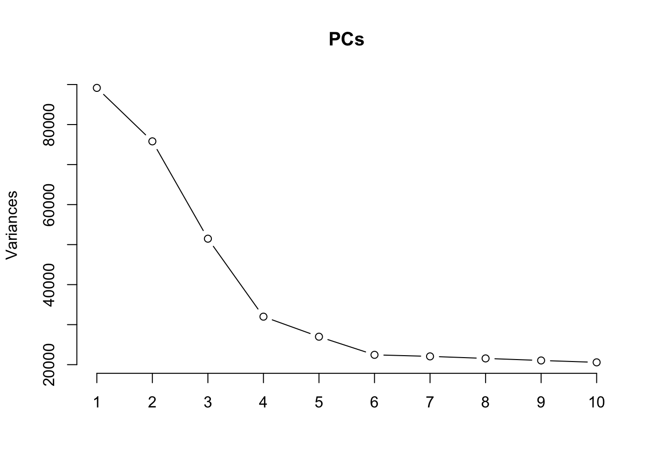
| Version | Author | Date |
|---|---|---|
| 2d78700 | JovMaksimovic | 2020-09-18 |
Collect all of the known sample traits.
nGenes = nrow(mValsNoXY)
nSamples = ncol(mValsNoXY[, runOne])
datTraits <- info %>% inner_join(rownames_to_column(data.frame(props$counts)),
                                 by = c("Sample_source" = "rowname")) %>%
  dplyr::select(-Sample_ID, -Sample_Group, -Sample_source, -Sample_run,
                -Basename, -ID) %>%
  mutate_at("BAL_Age", as.numeric) %>%
  mutate(Status = as.numeric(factor(Status, labels = 1:2)),
         Sex = as.numeric(factor(Sex, labels = 1:2))) %>%
  mutate_if(is.numeric, replace_na, 0)

head(datTraits)
Pair Status BAL_Age Sex BMI EpithelialCell Macrophage Granulocyte
1 1 1 6.02 1 16.93 0.02928789 0.7379693 0.1299190
2 1 2 6.12 1 14.76 0.02711103 0.6558064 0.2643458
3 2 1 6.05 1 14.94 0.11624431 0.3946144 0.4045330
4 2 2 5.89 1 16.69 0.11132203 0.4022755 0.3832535
5 3 1 6.05 1 20.00 0.07693852 0.6631655 0.1845067
6 3 2 6.05 1 19.82 0.06904478 0.0000000 0.8483914
Lymphocyte
1 0.11795500
2 0.06935392
3 0.13159166
4 0.14163820
5 0.09487492
6 0.08952296Correlate known sample traits with the top 20 principal components. This can help us determine which traits are potentially contributing to the main sources of variation in the data and should thus be included in our statistical analysis.
The correlation plot shows that differences in cell type proportions between samples are contributing to a lot of the variation in the top 3 principal components. Case/control status, pairing and age are potentially also contributing to the variation in the top few components. BMI and sex, however, seem to be only capturing a very small component of the variation.
moduleTraitCor <- suppressWarnings(cor(loadings[, 1:20], datTraits, use = "p"))
moduleTraitPvalue <- WGCNA::corPvalueStudent(moduleTraitCor, (nSamples-2))
textMatrix <- paste(signif(moduleTraitCor, 2), "\n(",
signif(moduleTraitPvalue, 1), ")", sep = "")
dim(textMatrix) <- dim(moduleTraitCor)
## Display the correlation values within a heatmap plot
par(cex=0.75, mar = c(6, 8.5, 3, 3))
WGCNA::labeledHeatmap(Matrix = t(moduleTraitCor),
xLabels = colnames(loadings)[1:20],
yLabels = names(datTraits),
colorLabels = FALSE,
colors = WGCNA::blueWhiteRed(6),
textMatrix = t(textMatrix),
setStdMargins = FALSE,
cex.text = 0.5,
zlim = c(-1,1),
main = paste("PCA-trait relationships: Top 20 PCs"))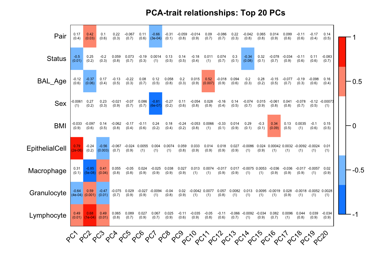
| Version | Author | Date |
|---|---|---|
| 2d78700 | JovMaksimovic | 2020-09-18 |
Visualising the variation
Examine the estimated cell type proportions, stratified by case/control pair. Pairs 1, 2, 5, 7, 10 and 11 show very similar cell type estimates across all cell types. The remaining pairs, 3, 4, 6, 8, 9, 12, 13 and 14 show some divergence in estimates between cases and controls, particularly for macrophages and granulocytes.
reshape2::melt(props$counts) %>%
  rename(sample = Var1, cell = Var2, prop = value) %>%
  inner_join(info, by = c("sample" = "Sample_source")) %>%
  dplyr::select(-Basename, -BAL_Age) -> dat

ggplot(dat, aes(x = cell, y = prop, colour = Sample_Group)) +
  geom_point(shape = 1) +
  facet_wrap(vars(Pair), ncol = 4, nrow = 4) +
  theme(axis.text.x = element_text(angle = 90, vjust = 0.5, hjust = 1)) +
  labs(x = "Cell Type", y = "Est. Proportion",
       colour = "Group")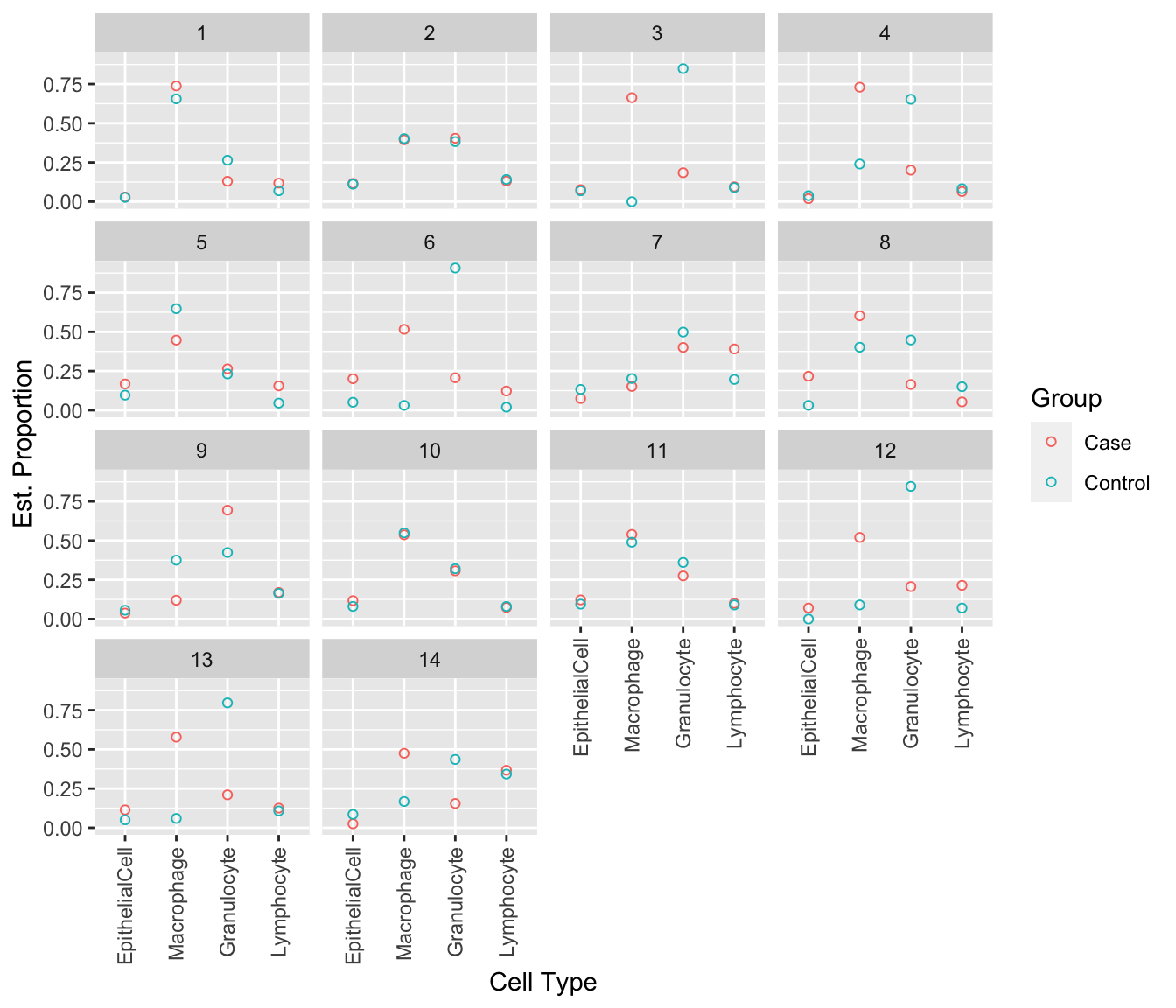
| Version | Author | Date |
|---|---|---|
| 2d78700 | JovMaksimovic | 2020-09-18 |
MDS plot coloured by estimated cell type proportions, stratified by cell type. As expected from the PCA-trait correlations, the clustering observed in the top 2 components appears to be driven by differences in cell type proportions, paritularly of macrophages and granulocytes.
mds <- plotMDS(mValsNoXY[, runOne], top = 1000, gene.selection="common",
               plot = FALSE)
dat %>% inner_join(tibble(x = mds$x,
                          y = mds$y,
                          Sample_ID = names(mds$x))) -> mdat
Joining, by = "Sample_ID"p <- ggplot(mdat, aes(x = x, y = y, colour = prop)) +
geom_text(aes(label = Pair), size = 2.7) +
facet_wrap(vars(cell), ncol = 2, nrow = 2) +
labs(colour = "Est. Proportion",
x = "Principal component 1",
y = "Principal component 2") +
ggtitle("Pairs (No XY probes)") +
scale_colour_viridis_c(option = "magma", direction = 1)
p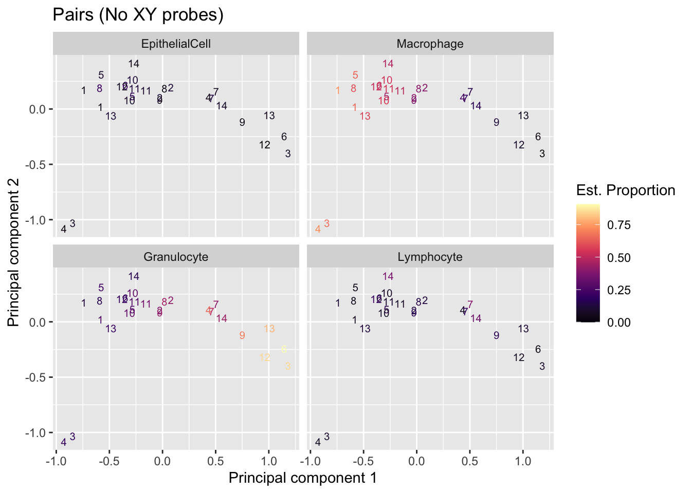
| Version | Author | Date |
|---|---|---|
| 2d78700 | JovMaksimovic | 2020-09-18 |
Is BMI important?
The controls appear to be more variable in their BMI than the cases. This potentially because the children with more severe disease tend to have lower BMI.
ggplot(info, aes(x = Status, y = BMI, fill = Status)) +
  geom_boxplot()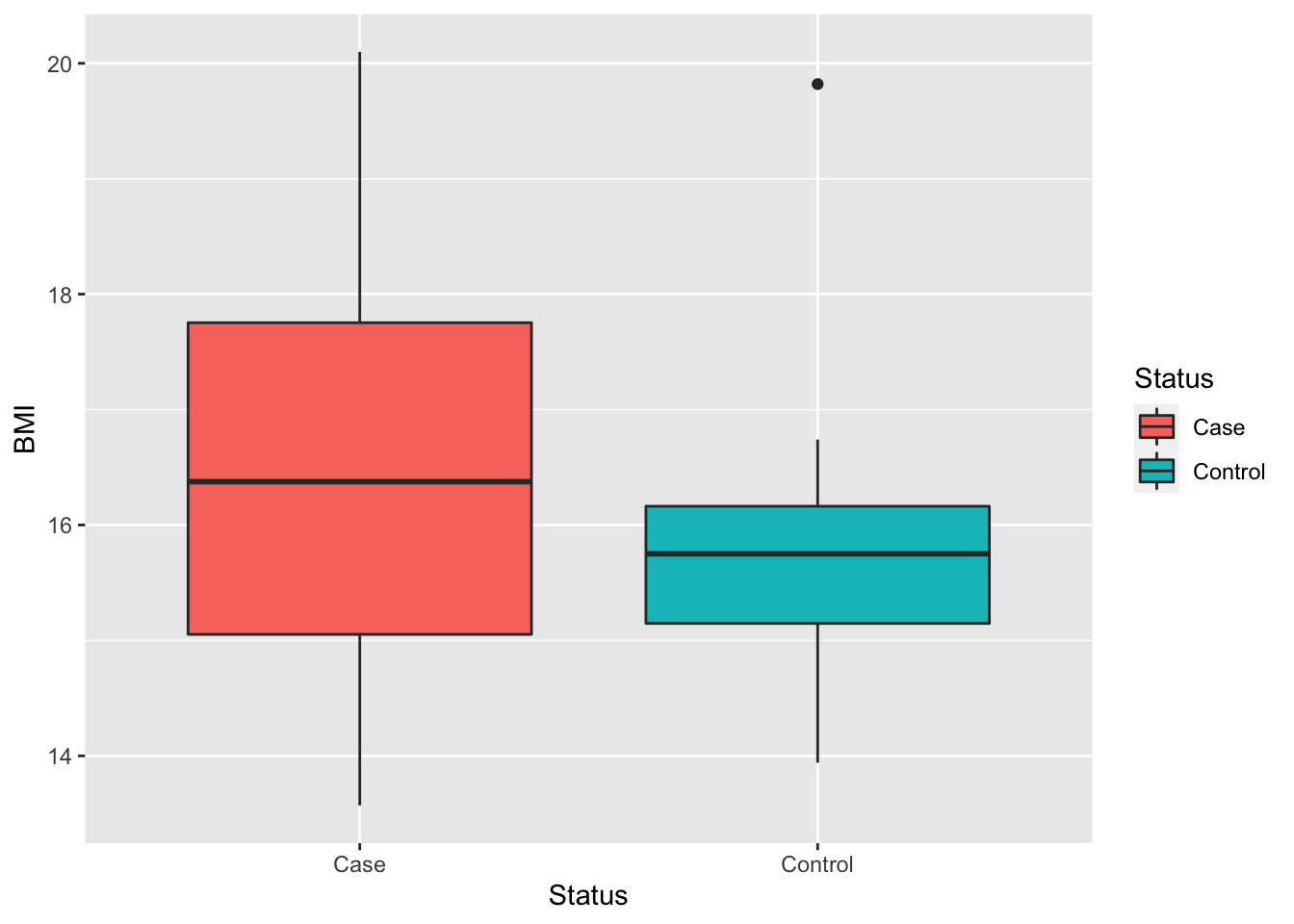
| Version | Author | Date |
|---|---|---|
| 2d78700 | JovMaksimovic | 2020-09-18 |
Population mean ranks are not significantly different between cases and controls.
wilcox.test(BMI ~ Status, data = info, paired = TRUE)Warning in wilcox.test.default(x = c(16.93, 14.94, 20, 19.37, 14.98, 16.41, :
cannot compute exact p-value with ties
    Wilcoxon signed rank test with continuity correction

data:  BMI by Status
V = 72.5, p-value = 0.2208
alternative hypothesis: true location shift is not equal to 0
Looking at BMI stratified by pair shows that some pairs have very little BMI difference, whilst some pairs have much larger differences in BMI.
p <- ggplot(info, aes(x = Pair, y = BMI, colour = Status)) +
  geom_point(shape = 1, size = 3) +
  scale_x_discrete(limits = factor(unique(info$Pair))) +
  labs(x = "Pair", y = "BMI", colour = "Status")
p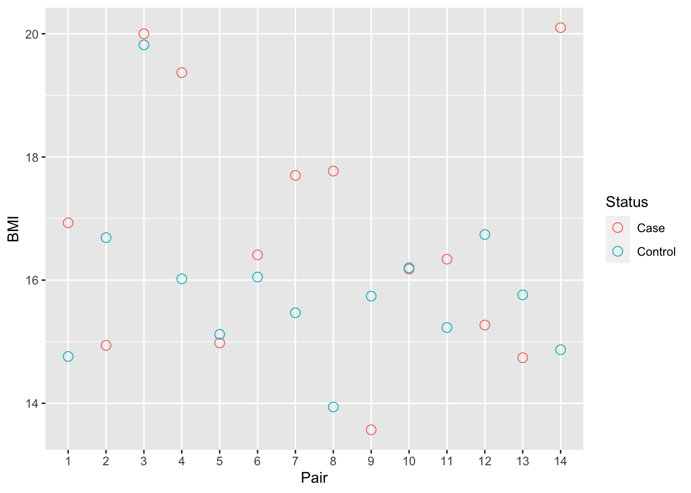
| Version | Author | Date |
|---|---|---|
| 2d78700 | JovMaksimovic | 2020-09-18 |
Compare distribution of adjusted R-squared values for model with (ALT) and without (NULL) BMI included across all CpGs.
cellEst <- data.frame(props$counts)
AEC <- cellEst$EpithelialCell
lymph <- cellEst$Lymphocyte
gran <- cellEst$Granulocyte
mac <- cellEst$Macrophage

out <- here("data/arsq.rds")

if(!file.exists(out)){
  bpparam <- MulticoreParam(multicoreWorkers() - 1)

  arsq <- bplapply(1:nrow(data), function(i){
    cpg <- data[i, ]
    null <- summary(lm(cpg ~ info$Status + info$Pair +
                         AEC + lymph + mac))$adj.r.squared
    alt <- summary(lm(cpg ~ info$Status + info$Pair +
                         AEC + lymph + mac + info$BMI))$adj.r.squared
    data.frame(arsq = c(null, alt),
               type = c("null", "alt"))
  }, BPPARAM = bpparam())
  names(arsq) <- rownames(data)
  arsq <- bind_rows(arsq, .id = "cpg")
  saveRDS(arsq, file = out)

} else {
  arsq <- readRDS(out)

}
Distributions are broadly similar.
ggplot(arsq, aes(x = arsq, fill = type)) +
  geom_histogram(position = "dodge") +
  labs(x = "Adj. R-squared", y = "No. CpGs",
       fill = "Model") +
  ggtitle("Distribution of Adj. R-squared Values")
`stat_bin()` using `bins = 30`. Pick better value with `binwidth`.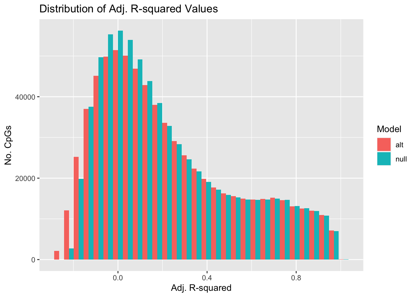
| Version | Author | Date |
|---|---|---|
| 2d78700 | JovMaksimovic | 2020-09-18 |
A slightly greater proportion of ALT models (~0.005) have an adjusted R-squared greater than 10%, indicating that including BMI may be an improvement.
arsq %>% group_by(type) %>%
  summarise(prop = sum(arsq > 0.1)/n())
`summarise()` ungrouping output (override with `.groups` argument)# A tibble: 2 x 2
type prop
<fct> <dbl>
1 alt 0.565
2 null 0.559Perform likelihood ratio test between NULL and ALT models for each CpG.
out <- here("data/loglrt.rds")

if(!file.exists(out)){
  bpparam <- MulticoreParam(multicoreWorkers() - 1)

  lrt <- bplapply(1:nrow(data), function(i){
    cpg <- data[i, ]
    null <- lm(cpg ~ info$Status + info$Pair + AEC + lymph + mac)
    alt <- lm(cpg ~ info$Status + info$Pair + AEC + lymph + mac + info$BMI)
    teststat <- -2 * (logLik(null) - logLik(alt))
    pval <- pchisq(teststat, df = 1, lower.tail = FALSE)
    as.numeric(pval)

  }, BPPARAM = bpparam())

  names(lrt) <- rownames(data)
  lrt <- unlist(lrt)

  saveRDS(lrt, file = out)

} else {
  lrt <- readRDS(out)

}
Including BMI significantly improves the model for ~63000 CpGs.
sum(lrt < 0.05)[1] 63307Although it appears that BMI only contributes to a relatively small amount of variation in this data, it will be included in the model as it does significantly improve the model for a number of CpGs.
Differential methylation analysis
Comparison of cases versus controls, taking into account pairing information and cell type proportions.
There are no statistically significant differences between cases and controls.
AEC <- cellEst$EpithelialCell
lymph <- cellEst$Lymphocyte
gran <- cellEst$Granulocyte
mac <- cellEst$Macrophage

design <- model.matrix(~0 + Status + Pair + AEC + lymph + gran + mac + BMI,
                       data = info)
colnames(design)[1:2] <- c("case", "control")

cont <- makeContrasts(caseVctrl = case - control,
                      levels = design)
fit <- lmFit(data, design)
cfit <- contrasts.fit(fit, cont)
fit2 <- eBayes(cfit, robust = TRUE)

summary(decideTests(fit2, p.value = 0.05))
caseVctrl
Down 0
NotSig 711147
Up 0These are the top 10 ranked CpGs.
data.frame(annEPIC) %>% dplyr::slice(match(rownames(fit2),
                                       rownames(annEPIC))) %>%
  dplyr::select(chr, pos, UCSC_RefGene_Name,
                UCSC_RefGene_Group) -> ann

top <- topTable(fit2, coef = "caseVctrl", genelist = ann, number = 100)
head(top, n = 10)
chr pos
cg08086906 chr16 86588932
cg14753740 chr5 54468940
cg05050482 chr6 30710482
cg09786634 chr17 78912393
cg09069203 chr1 214251836
cg06440065 chr19 30206617
cg23610373 chr1 149298587
cg03641032 chr17 78911768
cg11949518 chr17 78912765
cg24545338 chr14 31343687
UCSC_RefGene_Name
cg08086906 MTHFSD;MTHFSD;MTHFSD;MTHFSD;MTHFSD;MTHFSD;MTHFSD;FLJ30679
cg14753740 CDC20B;CDC20B;MIR449C;CDC20B;CDC20B;CDC20B;CDC20B
cg05050482 FLOT1
cg09786634 RPTOR;RPTOR
cg09069203
cg06440065 C19orf12;C19orf12
cg23610373
cg03641032 RPTOR;RPTOR
cg11949518 RPTOR;RPTOR
cg24545338 COCH;COCH
UCSC_RefGene_Group logFC
cg08086906 TSS200;TSS200;TSS200;TSS200;TSS200;TSS200;TSS200;Body -0.6312749
cg14753740 1stExon;1stExon;TSS1500;5'UTR;1stExon;5'UTR;5'UTR -1.1841422
cg05050482 TSS200 0.5974218
cg09786634 Body;Body -1.0748715
cg09069203 0.4528994
cg06440065 TSS200;TSS1500 -0.7147448
cg23610373 0.5430589
cg03641032 Body;Body -0.4436379
cg11949518 Body;Body -1.9388687
cg24545338 TSS200;TSS200 0.6874729
AveExpr t P.Value adj.P.Val B
cg08086906 -3.9721143 -5.963707 3.676186e-06 0.5787279 -0.1384698
cg14753740 -1.8155914 -5.904091 4.259512e-06 0.5787279 -0.1864078
cg05050482 -3.5470879 5.875938 4.566850e-06 0.5787279 -0.2092122
cg09786634 -1.3211280 -5.836888 5.030825e-06 0.5787279 -0.2410202
cg09069203 1.8458068 5.829601 5.098492e-06 0.5787279 -0.2443242
cg06440065 -2.4002866 -5.830922 5.105815e-06 0.5787279 -0.2458981
cg23610373 -2.6791507 5.738648 6.421410e-06 0.5787279 -0.3219518
cg03641032 0.8777105 -5.731297 6.510361e-06 0.5787279 -0.3254974
cg11949518 0.8334538 -5.681212 7.409210e-06 0.5854486 -0.3698704
cg24545338 -2.7777173 5.483738 1.214334e-05 0.7743650 -0.5379973These are the beta values of the top 9 ranked CpGs stratified by pair.
bdat <- reshape2::melt(bVals[, runOne])
bdat$pair <- rep(info$Pair, each = nrow(bVals))
bdat$group <- rep(info$Status, each = nrow(bVals))

p <- vector("list", 9)

for(i in 1:length(p)){
p[[i]] <- ggplot(data = subset(bdat, bdat$Var1 == rownames(top)[i]),
       aes(x = pair, y = value, colour = group)) +
  geom_jitter(width = 0.25) +
  scale_x_discrete(limits = factor(unique(bdat$pair))) +
  labs(x = "Pair", y = "Beta value", colour = "Status") +
  ggtitle(rownames(top)[i], subtitle = top$UCSC_RefGene_Name[i]) +
  theme(plot.title = element_text(size = 8),
        plot.subtitle = element_text(size = 7),
        axis.title = element_text(size = 8),
        axis.text.x = element_text(size = 7))
}

(p[[1]] | p[[2]] | p[[3]]) /
(p[[4]] | p[[5]] | p[[6]]) /
  (p[[7]] | p[[8]] | p[[9]]) +
  plot_layout(guides = "collect") & theme(legend.position = "bottom")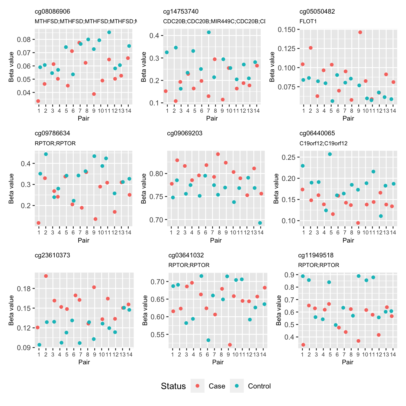
| Version | Author | Date |
|---|---|---|
| 2d78700 | JovMaksimovic | 2020-09-18 |
write.csv(top, file = here("output/case-ctrl-paired.csv"))
sessionInfo()R version 4.0.3 (2020-10-10)
Platform: x86_64-apple-darwin17.0 (64-bit)
Running under: macOS Mojave 10.14.6
Matrix products: default
BLAS: /Library/Frameworks/R.framework/Versions/4.0/Resources/lib/libRblas.dylib
LAPACK: /Library/Frameworks/R.framework/Versions/4.0/Resources/lib/libRlapack.dylib
locale:
[1] en_AU.UTF-8/en_AU.UTF-8/en_AU.UTF-8/C/en_AU.UTF-8/en_AU.UTF-8
attached base packages:
[1] stats4 parallel stats graphics grDevices utils datasets
[8] methods base
other attached packages:
[1] BiocParallel_1.24.1
[2] patchwork_1.1.1
[3] forcats_0.5.0
[4] stringr_1.4.0
[5] dplyr_1.0.2
[6] purrr_0.3.4
[7] readr_1.4.0
[8] tidyr_1.1.2
[9] tibble_3.0.4
[10] tidyverse_1.3.0
[11] ggplot2_3.3.2
[12] FlowSorted.Blood.EPIC_1.8.0
[13] ExperimentHub_1.16.0
[14] AnnotationHub_2.22.0
[15] BiocFileCache_1.14.0
[16] dbplyr_2.0.0
[17] nlme_3.1-151
[18] quadprog_1.5-8
[19] genefilter_1.72.0
[20] IlluminaHumanMethylationEPICmanifest_0.3.0
[21] missMethyl_1.24.0
[22] IlluminaHumanMethylationEPICanno.ilm10b4.hg19_0.6.0
[23] IlluminaHumanMethylation450kanno.ilmn12.hg19_0.6.0
[24] minfi_1.36.0
[25] bumphunter_1.32.0
[26] locfit_1.5-9.4
[27] iterators_1.0.13
[28] foreach_1.5.1
[29] Biostrings_2.58.0
[30] XVector_0.30.0
[31] SummarizedExperiment_1.20.0
[32] Biobase_2.50.0
[33] MatrixGenerics_1.2.0
[34] matrixStats_0.57.0
[35] GenomicRanges_1.42.0
[36] GenomeInfoDb_1.26.2
[37] IRanges_2.24.1
[38] S4Vectors_0.28.1
[39] BiocGenerics_0.36.0
[40] limma_3.46.0
[41] here_1.0.1
[42] workflowr_1.6.2
loaded via a namespace (and not attached):
[1] utf8_1.1.4 tidyselect_1.1.0
[3] htmlwidgets_1.5.3 RSQLite_2.2.1
[5] AnnotationDbi_1.52.0 grid_4.0.3
[7] munsell_0.5.0 codetools_0.2-18
[9] preprocessCore_1.52.0 statmod_1.4.35
[11] withr_2.3.0 colorspace_2.0-0
[13] knitr_1.30 rstudioapi_0.13
[15] labeling_0.4.2 git2r_0.27.1
[17] GenomeInfoDbData_1.2.4 bit64_4.0.5
[19] farver_2.0.3 rhdf5_2.34.0
[21] rprojroot_2.0.2 vctrs_0.3.6
[23] generics_0.1.0 xfun_0.19
[25] fastcluster_1.1.25 R6_2.5.0
[27] doParallel_1.0.16 illuminaio_0.32.0
[29] bitops_1.0-6 rhdf5filters_1.2.0
[31] reshape_0.8.8 DelayedArray_0.16.0
[33] assertthat_0.2.1 promises_1.1.1
[35] scales_1.1.1 nnet_7.3-14
[37] gtable_0.3.0 WGCNA_1.69
[39] rlang_0.4.9 splines_4.0.3
[41] rtracklayer_1.50.0 impute_1.64.0
[43] GEOquery_2.58.0 checkmate_2.0.0
[45] broom_0.7.3 reshape2_1.4.4
[47] BiocManager_1.30.10 yaml_2.2.1
[49] modelr_0.1.8 GenomicFeatures_1.42.1
[51] backports_1.2.1 httpuv_1.5.4
[53] Hmisc_4.4-2 tools_4.0.3
[55] nor1mix_1.3-0 ellipsis_0.3.1
[57] RColorBrewer_1.1-2 siggenes_1.64.0
[59] dynamicTreeCut_1.63-1 Rcpp_1.0.5
[61] plyr_1.8.6 base64enc_0.1-3
[63] sparseMatrixStats_1.2.0 progress_1.2.2
[65] zlibbioc_1.36.0 RCurl_1.98-1.2
[67] prettyunits_1.1.1 rpart_4.1-15
[69] openssl_1.4.3 cluster_2.1.0
[71] haven_2.3.1 fs_1.5.0
[73] magrittr_2.0.1 data.table_1.13.4
[75] reprex_0.3.0 whisker_0.4
[77] hms_0.5.3 mime_0.9
[79] evaluate_0.14 xtable_1.8-4
[81] XML_3.99-0.5 jpeg_0.1-8.1
[83] mclust_5.4.7 readxl_1.3.1
[85] gridExtra_2.3 compiler_4.0.3
[87] biomaRt_2.46.0 crayon_1.3.4
[89] htmltools_0.5.0 later_1.1.0.1
[91] Formula_1.2-4 lubridate_1.7.9.2
[93] DBI_1.1.0 MASS_7.3-53
[95] rappdirs_0.3.1 Matrix_1.2-18
[97] cli_2.2.0 pkgconfig_2.0.3
[99] GenomicAlignments_1.26.0 foreign_0.8-80
[101] xml2_1.3.2 annotate_1.68.0
[103] rngtools_1.5 multtest_2.46.0
[105] beanplot_1.2 rvest_0.3.6
[107] doRNG_1.8.2 scrime_1.3.5
[109] digest_0.6.27 rmarkdown_2.6
[111] base64_2.0 cellranger_1.1.0
[113] htmlTable_2.1.0 DelayedMatrixStats_1.12.1
[115] curl_4.3 shiny_1.5.0
[117] Rsamtools_2.6.0 lifecycle_0.2.0
[119] jsonlite_1.7.2 Rhdf5lib_1.12.0
[121] viridisLite_0.3.0 askpass_1.1
[123] fansi_0.4.1 pillar_1.4.7
[125] lattice_0.20-41 fastmap_1.0.1
[127] httr_1.4.2 survival_3.2-7
[129] GO.db_3.12.1 interactiveDisplayBase_1.28.0
[131] glue_1.4.2 png_0.1-7
[133] BiocVersion_3.12.0 bit_4.0.4
[135] stringi_1.5.3 HDF5Array_1.18.0
[137] blob_1.2.1 org.Hs.eg.db_3.12.0
[139] latticeExtra_0.6-29 memoise_1.1.0