Paedriatic airway atlas: all Tissues
Quality control: Exploratory Plots
Gunjan Dixit and Jovana Maksimovic
August 15, 2023
Last updated: 2023-08-15
Checks: 7 0
Knit directory: paed-airway-allTissues/
This reproducible R Markdown analysis was created with workflowr (version 1.7.0). The Checks tab describes the reproducibility checks that were applied when the results were created. The Past versions tab lists the development history.
Great! Since the R Markdown file has been committed to the Git repository, you know the exact version of the code that produced these results.
Great job! The global environment was empty. Objects defined in the global environment can affect the analysis in your R Markdown file in unknown ways. For reproduciblity it’s best to always run the code in an empty environment.
The command set.seed(20230811) was run prior to running
the code in the R Markdown file. Setting a seed ensures that any results
that rely on randomness, e.g. subsampling or permutations, are
reproducible.
Great job! Recording the operating system, R version, and package versions is critical for reproducibility.
Nice! There were no cached chunks for this analysis, so you can be confident that you successfully produced the results during this run.
Great job! Using relative paths to the files within your workflowr project makes it easier to run your code on other machines.
Great! You are using Git for version control. Tracking code development and connecting the code version to the results is critical for reproducibility.
The results in this page were generated with repository version baf913b. See the Past versions tab to see a history of the changes made to the R Markdown and HTML files.
Note that you need to be careful to ensure that all relevant files for
the analysis have been committed to Git prior to generating the results
(you can use wflow_publish or
wflow_git_commit). workflowr only checks the R Markdown
file, but you know if there are other scripts or data files that it
depends on. Below is the status of the Git repository when the results
were generated:
Ignored files:
    Ignored:    .Rhistory
    Ignored:    .Rproj.user/
    Ignored:    data/RDS/
    Ignored:    output/G000231_Neeland_batch1/
    Ignored:    output/G000231_Neeland_batch2_1/
    Ignored:    output/G000231_Neeland_batch2_2/
    Ignored:    output/G000231_Neeland_batch3/
    Ignored:    output/G000231_Neeland_batch4/
    Ignored:    output/G000231_Neeland_batch5/

Untracked files:
    Untracked:  figure/

Unstaged changes:
    Deleted:    02_QC_exploratoryPlots.Rmd
    Deleted:    02_QC_exploratoryPlots.html
Note that any generated files, e.g. HTML, png, CSS, etc., are not included in this status report because it is ok for generated content to have uncommitted changes.
These are the previous versions of the repository in which changes were
made to the R Markdown
(analysis/02_QC_exploratoryPlots.Rmd) and HTML
(docs/02_QC_exploratoryPlots.html) files. If you’ve
configured a remote Git repository (see ?wflow_git_remote),
click on the hyperlinks in the table below to view the files as they
were in that past version.
| File | Version | Author | Date | Message |
|---|---|---|---|---|
| Rmd | baf913b | Gunjan Dixit | 2023-08-15 | wflow_publish("analysis/*") |
Introduction
This RMarkdown contains exploratory plots to determine the quality of scRNA-seq data obtained from healthy tissue samples from five key locations of the respiratory system in children. The aim of this project is to develop a cell atlas of the healthy pediatric airway.
Load libraries
suppressPackageStartupMessages({
  library(BiocStyle)
  library(tidyverse)
  library(here)
  library(glue)
  library(RColorBrewer)
  library(scran)
  library(scater)
  library(scuttle)
  library(janitor)
  library(cowplot)
  library(patchwork)
  library(scales)
  library(Homo.sapiens)
  library(msigdbr)
  library(EnsDb.Hsapiens.v86)
  library(ensembldb)
})
Load data
List the batches.
Batch 1- Nasal brushings (n=16)
Batch
2_1- Tonsils (n=16)
Batch 2_2- Nasal
brushings (n=9) (repeats)
Batch 3- Adenoids (n=16)
Batch 4- Bronchial brushings (n=16)
Batch 5- Nasal brushings (n=16)
tissue_types <- c("Nasal_brushings", "Tonsils", "Nasal_brushings_repeat", "Adenoids", "Bronchial_brushings", "Nasal_brushings_2")
batches <- dir(here("output"), include.dirs = FALSE, pattern = "G000231_Neeland")
batches
[1] "G000231_Neeland_batch1" "G000231_Neeland_batch2_1"
[3] "G000231_Neeland_batch2_2" "G000231_Neeland_batch3"
[5] "G000231_Neeland_batch4" "G000231_Neeland_batch5" Non-empty droplets
Read non-empty droplets for each batch and summarize them together using bar plot.
# Initialize a list to store the plots
plot_list <- list()

for (batch_name in batches) {
  batch_files <- list.files(
    path = here("output", batch_name, "RDS", "SCEs"),
    pattern = "\\.emptyDrops\\.SCE\\.rds$",
    full.names = TRUE)
  sce <- readRDS(batch_files)

  num_unique_samples <- length(unique(sce$Sample))
color_palette <- colorRampPalette(brewer.pal(20, "Set3"))(num_unique_samples)

  # Extract unique sample names and assign colors from the color palette
  names(color_palette) <- sort(unique(sce$Sample))

  # Create the plot for the current batch
  p <- ggcells(sce) +
    geom_bar(aes(x = Sample, fill = Sample)) +
    coord_flip() +
    ylab("Number of droplets") +
    theme_cowplot(font_size = 10) +
    geom_text(stat='count', aes(x = Sample, label=..count..), hjust=1.5, size=3) +
    guides(fill = "none") +
    scale_fill_manual(values = color_palette) +
    labs(title = batch_name)

  # Store the plot in the list
  plot_list[[batch_name]] <- p
}
Plot number of non-empty droplets in each batch.
for (i in seq_along(batches)){
  batch_name <- batches[i]
  tissue_type <- tissue_types[i]
  cat('### ', batch_name, " - ", tissue_type, '\n')
  print(plot_list[[batch_name]])
  cat('\n\n')
}
G000231_Neeland_batch1 - Nasal_brushings
![]()
G000231_Neeland_batch2_1 - Tonsils
![]()
G000231_Neeland_batch2_2 - Nasal_brushings_repeat
![]()
G000231_Neeland_batch3 - Adenoids
![]()
G000231_Neeland_batch4 - Bronchial_brushings
![]()
G000231_Neeland_batch5 - Nasal_brushings_2
![]()
Quality control
Define the quality control metrics
Low-quality cells need to be removed to ensure that technical effects do not distort downstream analysis results. We use several quality control (QC) metrics to measure the quality of the cells:
sum: This measures the library size of the cells, which is the total sum of counts across both genes and spike-in transcripts. We want cells to have high library sizes as this means more RNA has been successfully captured during library preparation.detected: This is the number of expressed features. The number of expressed features refers to the number of genes which have non-zero counts (i.e. they have been identified in the cell at least once) in each cell. Cells with few expressed features are likely to be of poor quality, as the diverse transcript population has not been successful captured.subsets_Mito_percent: This measures the proportion of UMIs which are mapped to mitochondrial RNA. If there is a higher than expected proportion of mitochondrial RNA this is often symptomatic of a cell which is under stress and is therefore of low quality and will not be used for the analysis.subsets_Ribo_percent: This measures the proportion of UMIs which are mapped to ribosomal protein genes. If there is a higher than expected proportion of ribosomal protein gene expression this is often symptomatic of a cell which is of compromised quality and we may want to exclude it from the analysis.
Quality control using Scater
Here, we employ the Scater package to perform quality control (QC) on the single-cell RNA sequencing data. To enhance the interpretability of the data, we begin by converting ENSEMBL IDs to gene names using annotation databases from Bioconductor.
Function to add gene-based annotation
add_geneAnno <- function(sce){
  # Set rownames to avoid duplicate IDs
  rownames(sce) <- uniquifyFeatureNames(rowData(sce)$ID, rowData(sce)$Symbol)
  # Add chromosome location so we can filter on mitochondrial genes.
location <- mapIds(
  x = EnsDb.Hsapiens.v86,
  # NOTE: Need to remove gene version number prior to lookup.
  keys = rowData(sce)$ID,
  keytype = "GENEID",
  column = "SEQNAME", warn = FALSE)
rowData(sce)$CHR <- location
# Additional gene metadata from ENSEMBL and NCBI
# NOTE: These columns were customised for this project.
ensdb_columns <- c(
  "GENEBIOTYPE", "GENENAME", "GENESEQSTART", "GENESEQEND", "SEQNAME", "SYMBOL")
names(ensdb_columns) <- paste0("ENSEMBL.", ensdb_columns)
stopifnot(all(ensdb_columns %in% columns(EnsDb.Hsapiens.v86)))
ensdb_df <- DataFrame(
  lapply(ensdb_columns, function(column) {
    mapIds(
      x = EnsDb.Hsapiens.v86,
      keys = rowData(sce)$ID,
      keytype = "GENEID",
      column = column,
      multiVals = "CharacterList")
  }),
  row.names = rowData(sce)$ID)
# NOTE: Can't look up GENEID column with GENEID key, so have to add manually.
ensdb_df$ENSEMBL.GENEID <- rowData(sce)$ID
# NOTE: Homo.sapiens combines org.Hs.eg.db and
#       TxDb.Hsapiens.UCSC.hg19.knownGene (as well as others) and therefore
#       uses entrez gene and RefSeq based data.

# NOTE: These columns were customised for this project.
ncbi_columns <- c(
  # From TxDB: None required
  # From OrgDB
  "ALIAS", "ENTREZID", "GENENAME", "REFSEQ", "SYMBOL")
names(ncbi_columns) <- paste0("NCBI.", ncbi_columns)
stopifnot(all(ncbi_columns %in% columns(Homo.sapiens)))
ncbi_df <- DataFrame(
  lapply(ncbi_columns, function(column) {
    mapIds(
      x = Homo.sapiens,
      keys = rowData(sce)$ID,
      keytype = "ENSEMBL",
      column = column,
      multiVals = "CharacterList")
  }),
  row.names = rowData(sce)$ID)
rowData(sce) <- cbind(rowData(sce), ensdb_df, ncbi_df)
# Some useful gene sets
mito_set <- rownames(sce)[which(rowData(sce)$CHR == "MT")]
ribo_set <- grep("^RP(S|L)", rownames(sce), value = TRUE)
# NOTE: A more curated approach for identifying ribosomal protein genes
#       (https://github.com/Bioconductor/OrchestratingSingleCellAnalysis-base/blob/ae201bf26e3e4fa82d9165d8abf4f4dc4b8e5a68/feature-selection.Rmd#L376-L380)

c2_sets <- msigdbr(species = "Homo sapiens", category = "C2")
ribo_set <- union(
  ribo_set,
  c2_sets[c2_sets$gs_name == "KEGG_RIBOSOME", ]$human_gene_symbol)
sex_set <- rownames(sce)[any(rowData(sce)$ENSEMBL.SEQNAME %in% c("X", "Y"))]
pseudogene_set <- rownames(sce)[
  any(grepl("pseudogene", rowData(sce)$ENSEMBL.GENEBIOTYPE))]
is_mito <- rownames(sce) %in% mito_set
is_ribo <- rownames(sce) %in% ribo_set

  return(list(is_ribo = is_ribo, is_mito = is_mito))
}
Following this, we proceed to apply the quality control metrics using the Scater/Scuttle package.
This function reads previously processed “emptyDrops” file for each
batch, adds gene-based annotation and uses addPerCellQC
function to compute per-cell QC statistics. It appends these statistics
to the colData of the SingleCellExperiment object, allowing us to retain
all relevant information in a single object for later manipulation.
# Function to run  for each batch
run_scater <- function(batch_name) {
  batch_files <- list.files(
    path = here("output", batch_name, "RDS", "SCEs"),
    pattern = "\\.emptyDrops\\.SCE\\.rds$",
    full.names = TRUE)
  sce <- readRDS(batch_files)
  num_unique_samples <- length(unique(sce$Sample))
  color_palette <- colorRampPalette(brewer.pal(20, "Set3"))(num_unique_samples)

  # Extract unique sample names and assign colors from the color palette
  names(color_palette) <- sort(unique(sce$Sample))

  gene_annot <- add_geneAnno(sce)
  is_ribo <- gene_annot$is_ribo
  is_mito <- gene_annot$is_mito

  sce <- addPerCellQC(
  sce,
  subsets = list(Mito = which(is_mito), Ribo = which(is_ribo)))
  sce$zero_pct <- colMeans(counts(sce) == 0)*100

# Save the output SingleCellExperiment object
  out <- here("output", batch_name, "RDS", "SCEs", paste0(batch_name, ".ScaterQC.SCE.rds"))
  if (!file.exists(out)) saveRDS(sce, file = out)
}

# Loop through each batch and process the samples
for (batch_name in batches) {
  run_scater(batch_name)
}
Subsequently, we list all the processed SingleCellExperiment (SCE) objects and visualize exploratory plots for each batch.
all_sce <- list()

for (batch_name in batches) {
  batch_file <- here("output", batch_name, "RDS", "SCEs", paste0(batch_name, ".ScaterQC.SCE.rds"))
  sce <- readRDS(batch_file)
  all_sce[[batch_name]] <- sce
}
Visualize QC plots for each batch
Before proceeding with the actual cell filtering process, we delve
into the distribution of the metrics among the droplets. To visualize
these distributions for each sample, we utilize the
plotColData function from the scater package, which
generates plots offering insights into these distributions.
Function to generate QC plots and metrics.
medians_list <- list()
generate_qc_plots <- function(sce, batch_name) {
  p1 <- plotColData(
    sce,
    "sum",
    x = "Sample",
    colour_by = "Sample",
    point_size = 0.5) +
    scale_y_log10() +
    annotation_logticks(
      sides = "l",
      short = unit(0.03, "cm"),
      mid = unit(0.06, "cm"),
      long = unit(0.09, "cm"))

  p2 <- plotColData(
    sce,
    "detected",
    x = "Sample",
    colour_by = "Sample",
    point_size = 0.5)

  p3 <- plotColData(
    sce,
    "subsets_Mito_percent",
    x = "Sample",
    colour_by = "Sample",
    point_size = 0.5)

  p4 <- plotColData(
    sce,
    "subsets_Ribo_percent",
    x = "Sample",
    colour_by = "Sample",
    point_size = 0.5)

  p5 <- plotColData(
    sce,
    "zero_pct",
    x = "Sample",
    colour_by = "Sample",
    point_size = 0.5)

  qc_plots <- p1 + p2 + p3 + p4 + p5 + plot_layout(guides = "collect", ncol = 2) &
    theme(legend.position = "none",
          axis.text.x = element_text(angle = 90, hjust = 1, vjust = 0))

  # Calculate the median values for each metric
  median_library_size <- median(sce$sum)
  median_genes_detected <- median(sce$detected)
  median_mito_percent <- median(sce$subsets_Mito_percent)

  # Add the median values to the list
  medians_list[[batch_name]] <- c(
    Library_Size_Median = median_library_size,
    Genes_Detected_Median = median_genes_detected,
    Mitochondrial_Percent_Median = median_mito_percent
  )

  # Convert the list to a data frame
  medians_df <- as.data.frame(do.call(rbind, medians_list))
  medians_df$Batch <- names(medians_list)

  # Return the list of plots and the median data frame
  return(list(qc_plots = qc_plots, medians_df = medians_df))
}
Call function for each batch and generate QC plots
# Call run_scater for each batch
for (i in seq_along(batches)){
  batch_name <- batches[i]
  tissue_type <- tissue_types[i]
  cat('### ', batch_name, " - ", tissue_type, '\n')
  sce <- all_sce[[i]]
  qc_plots_data <- generate_qc_plots(sce, batch_name)
  qc_plots <- qc_plots_data$qc_plots
  medians_df <- qc_plots_data$medians_df
  # Print the median values for each metric
  cat("Batch:", batch_name, " - ", tissue_type, "\n")
  print(qc_plots)
  cat("- The median library size is around", number(medians_df$Library_Size_Median, accuracy = 100, big.mark = ","), "\n")
  cat("- The median number of genes detected is around", number(medians_df$Genes_Detected_Median, accuracy = 100, big.mark = ","), "\n")
  cat("- The median percentage of UMIs that are mapped to mitochondrial RNA is around",
      percent(medians_df$Mitochondrial_Percent_Median, scale = 1), "\n")

  cat('\n\n')
}
G000231_Neeland_batch1 - Nasal_brushings
Batch: G000231_Neeland_batch1 - Nasal_brushings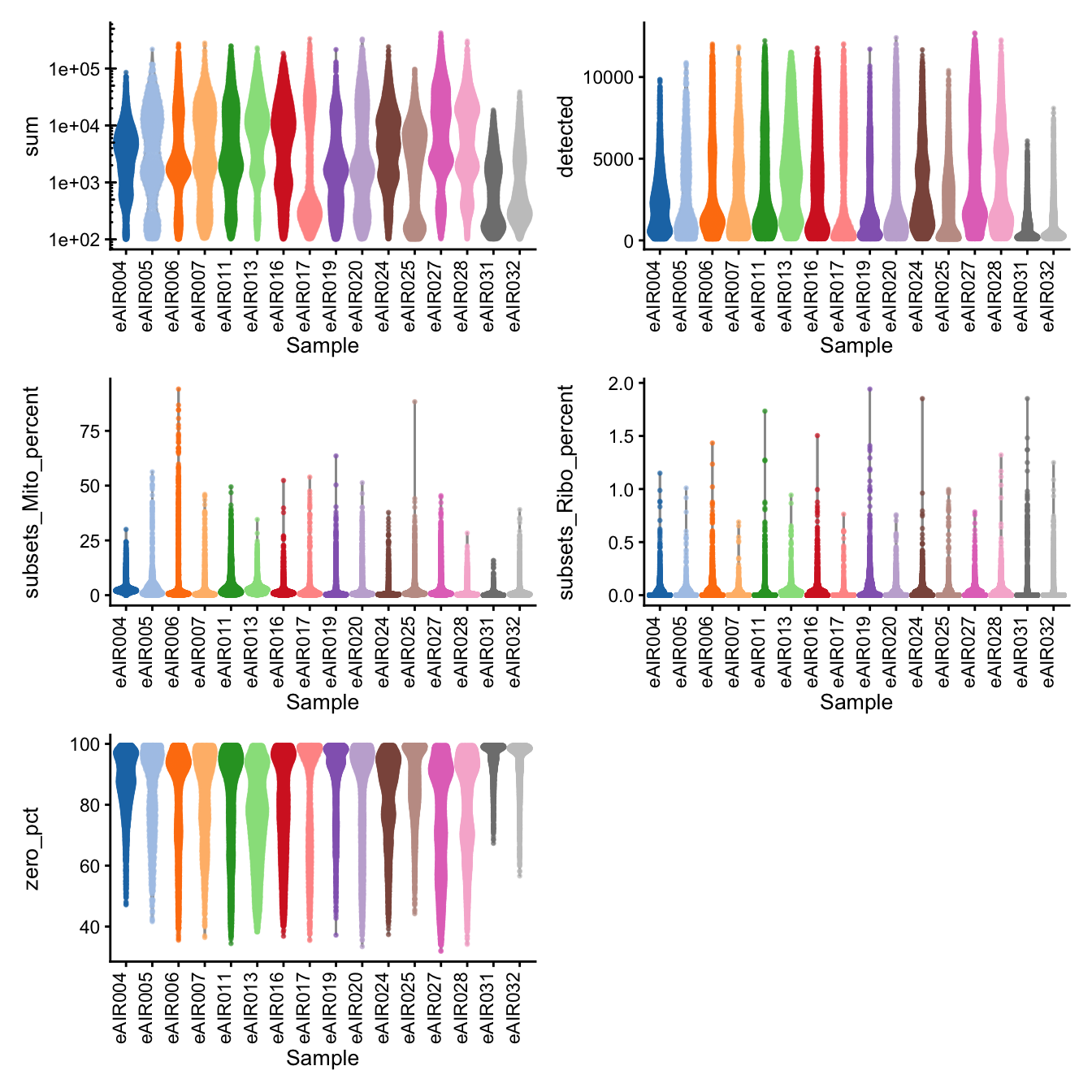
Distributions of various QC metrics
- The median library size is around 3,000
- The median number of genes detected is around 1,900
- The median percentage of UMIs that are mapped to mitochondrial RNA is around 1%
G000231_Neeland_batch2_1 - Tonsils
Batch: G000231_Neeland_batch2_1 - Tonsils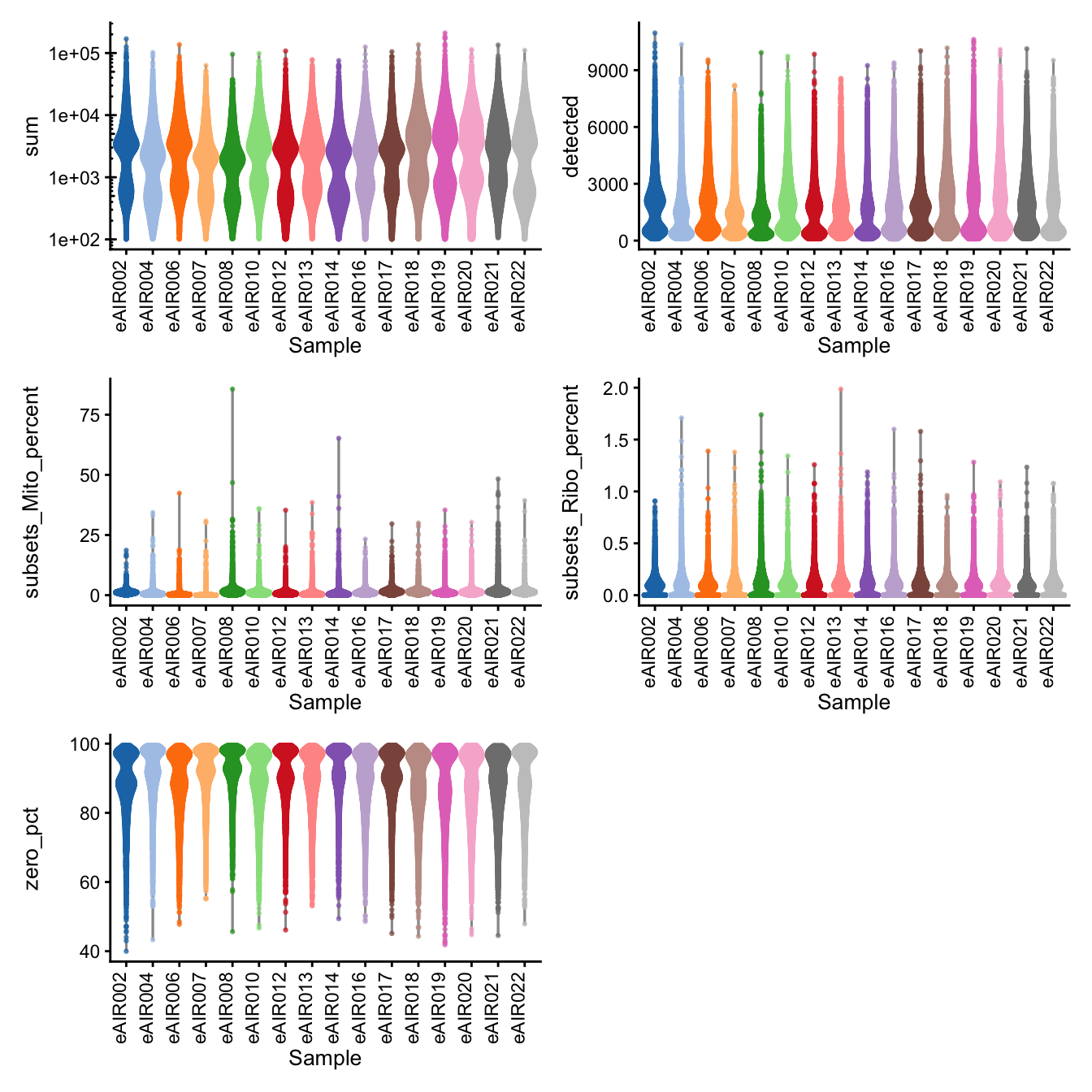
Distributions of various QC metrics
- The median library size is around 2,300
- The median number of genes detected is around 1,600
- The median percentage of UMIs that are mapped to mitochondrial RNA is around 1%
G000231_Neeland_batch2_2 - Nasal_brushings_repeat
Batch: G000231_Neeland_batch2_2 - Nasal_brushings_repeat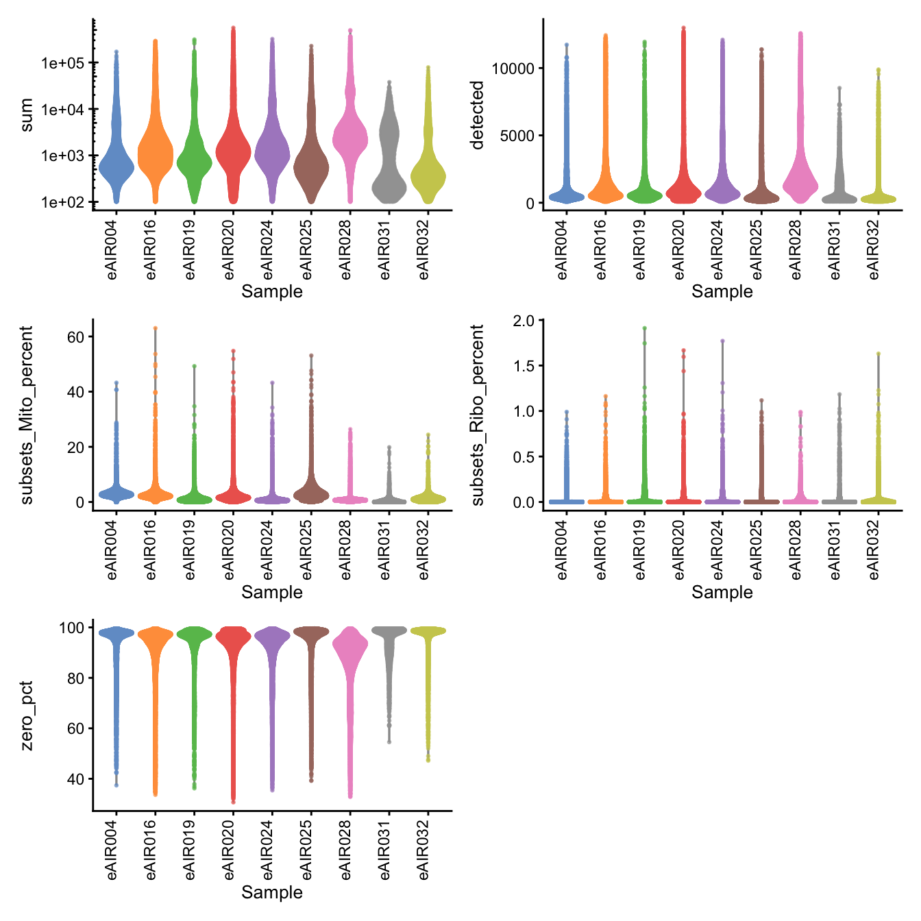
Distributions of various QC metrics
- The median library size is around 1,100
- The median number of genes detected is around 900
- The median percentage of UMIs that are mapped to mitochondrial RNA is around 1%
G000231_Neeland_batch3 - Adenoids
Batch: G000231_Neeland_batch3 - Adenoids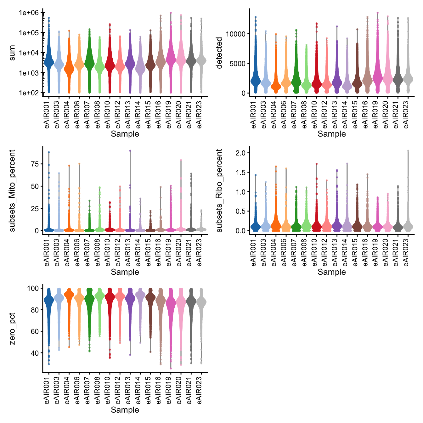
Distributions of various QC metrics
- The median library size is around 3,300
- The median number of genes detected is around 2,000
- The median percentage of UMIs that are mapped to mitochondrial RNA is around 1%
G000231_Neeland_batch4 - Bronchial_brushings
Batch: G000231_Neeland_batch4 - Bronchial_brushings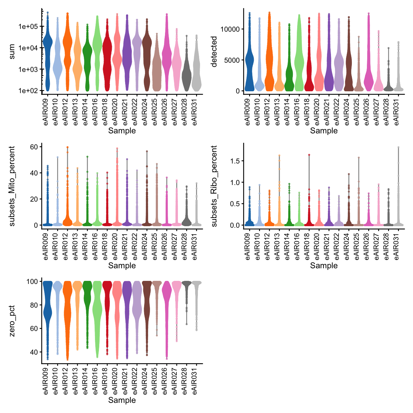
Distributions of various QC metrics
- The median library size is around 2,900
- The median number of genes detected is around 1,700
- The median percentage of UMIs that are mapped to mitochondrial RNA is around 1%
G000231_Neeland_batch5 - Nasal_brushings_2
Batch: G000231_Neeland_batch5 - Nasal_brushings_2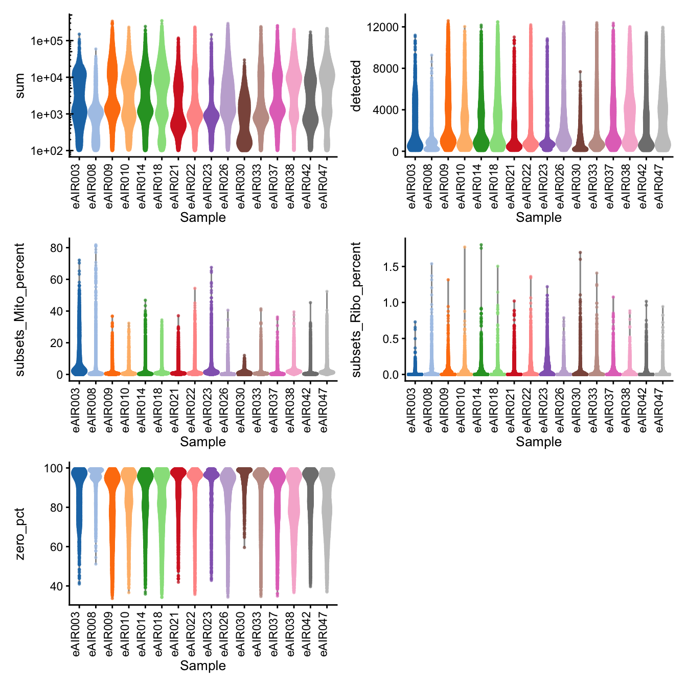
Distributions of various QC metrics
- The median library size is around 1,900
- The median number of genes detected is around 1,300
- The median percentage of UMIs that are mapped to mitochondrial RNA is around 1%
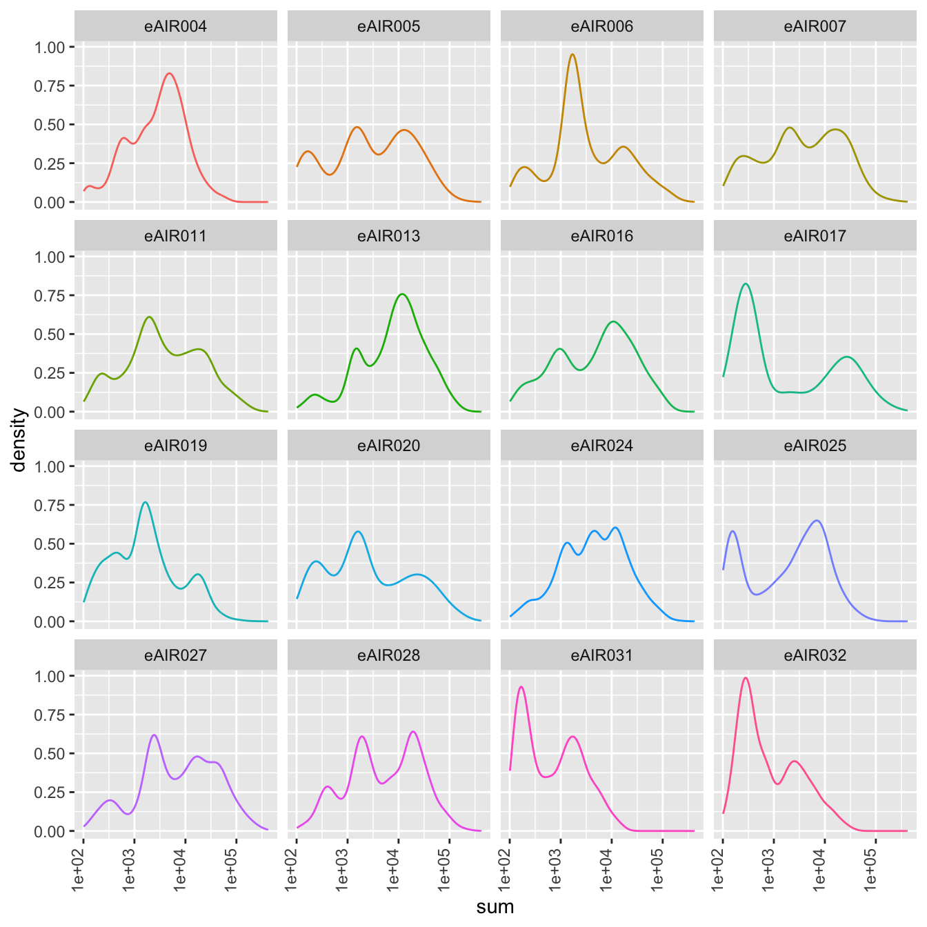
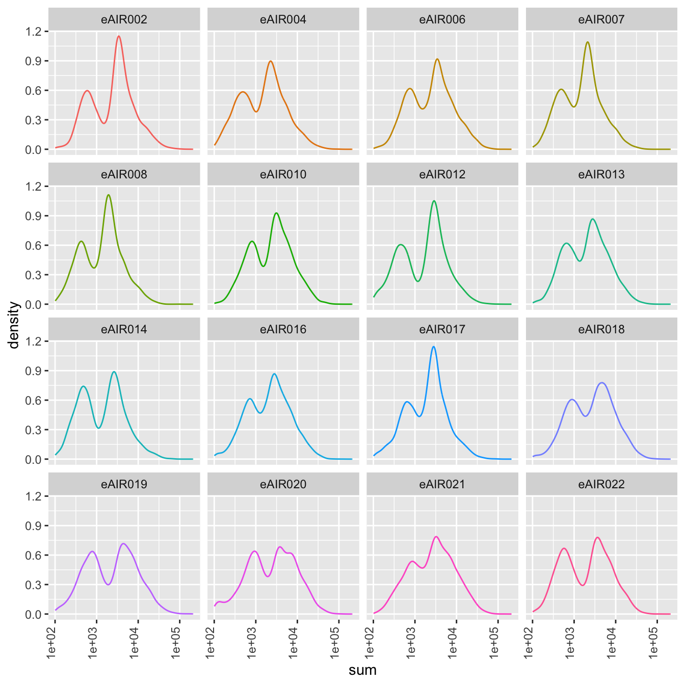
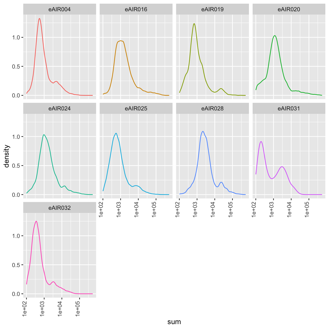
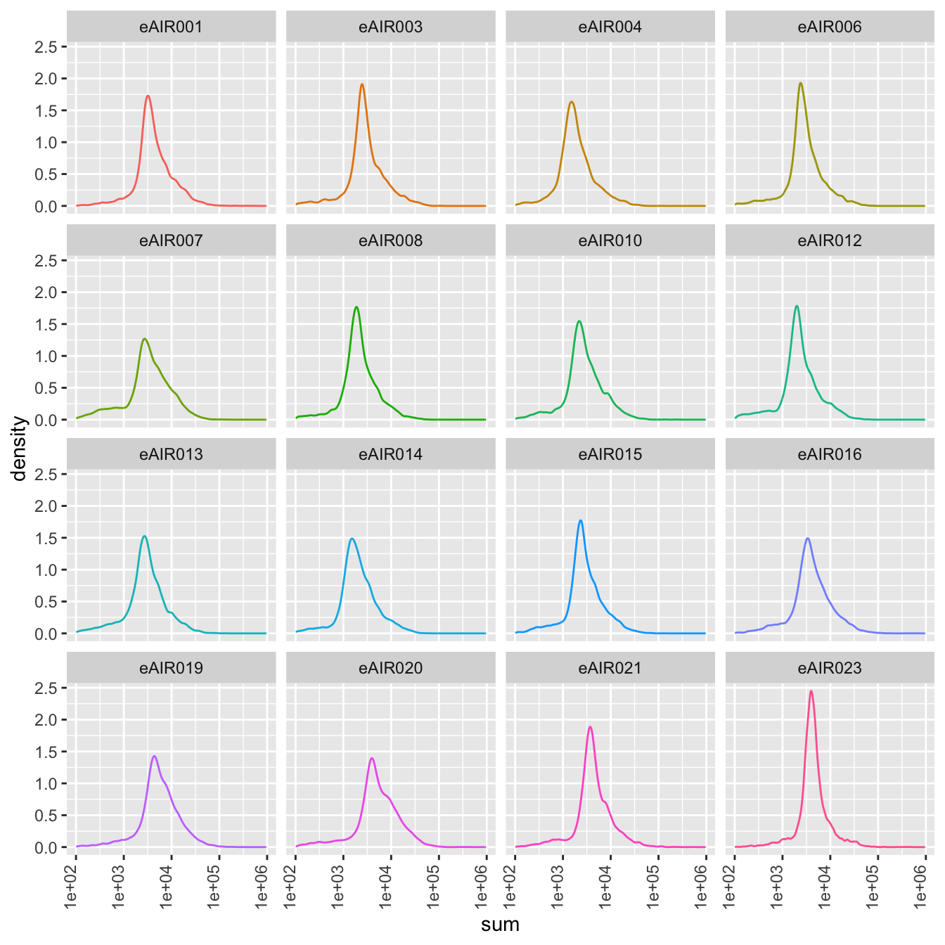
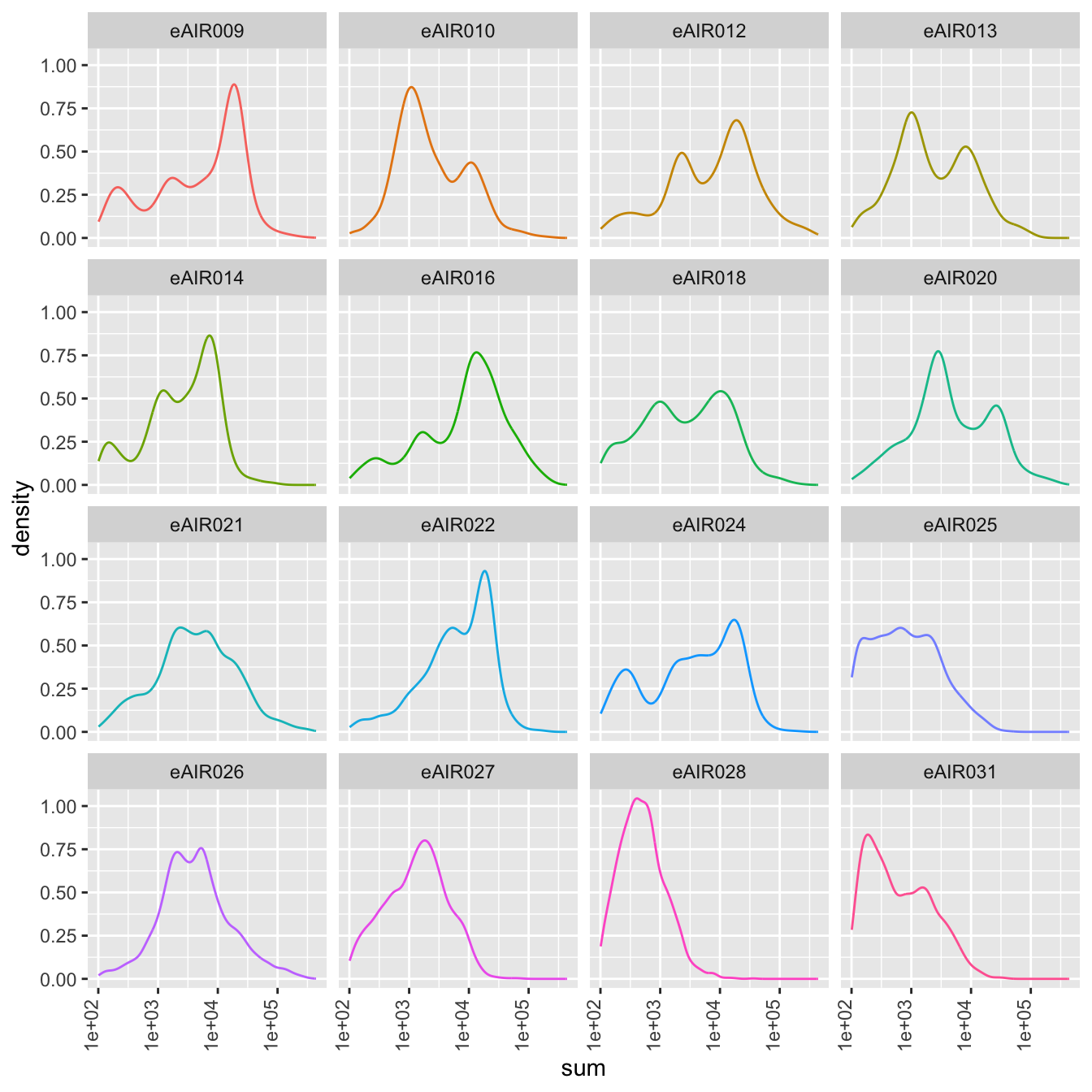
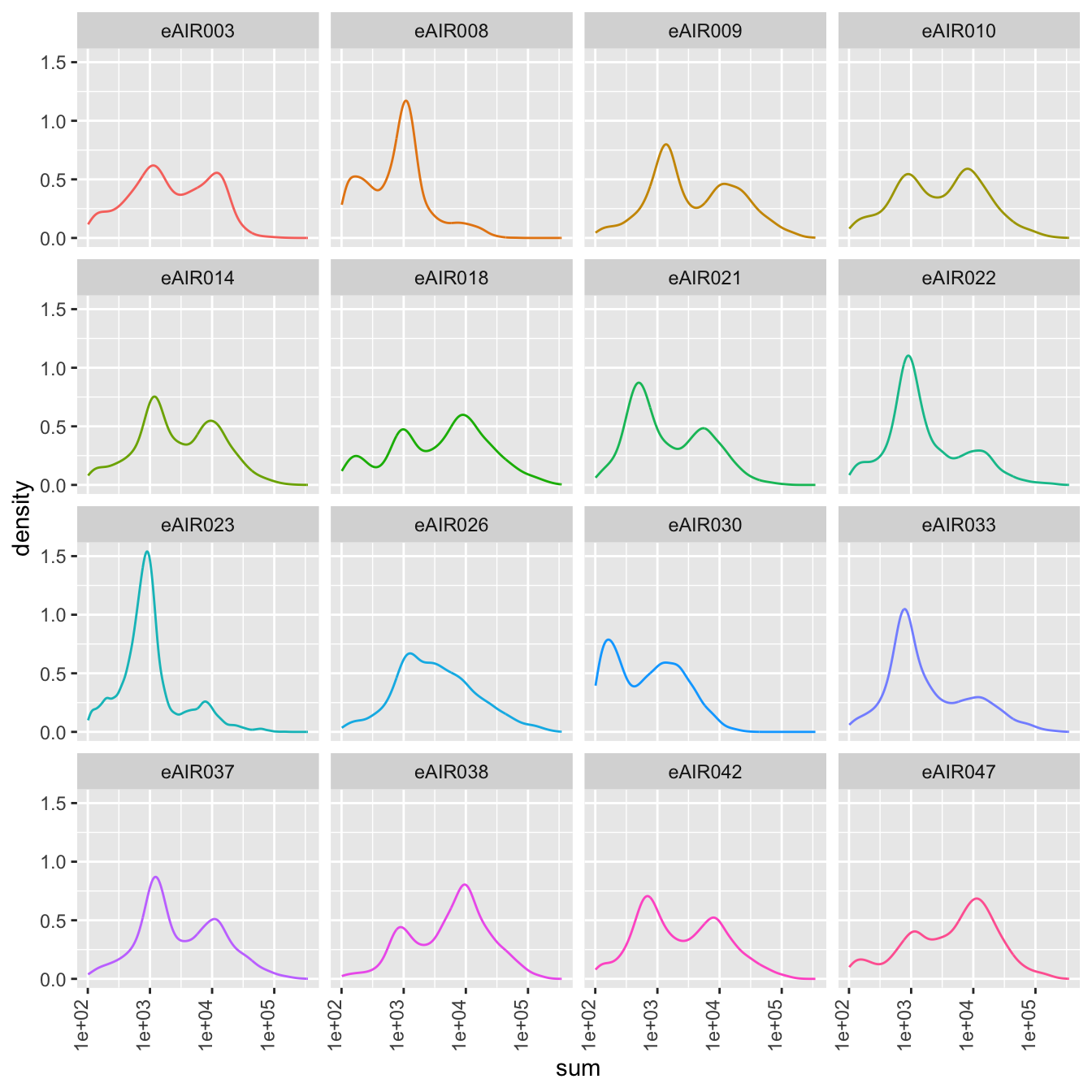
Density Plots
Here, density plot of the distribution of library sizes (sums of counts) across different samples is shown in each batch. It provides insights into the spread and concentration of data points across different samples. The shape and characteristics of the plot reveals information about the data distribution, such as whether the library sizes are centered around a specific value or whether there are multiple modes in the distribution.
for (i in seq_along(batches)){
  batch_name <- batches[i]
  tissue_type <- tissue_types[i]
  cat('### ', batch_name, " - ", tissue_type, '\n')
  sce <- all_sce[[i]]
  d <- colData(sce) %>%
  data.frame %>%
  ggplot(aes(x = sum, colour = Sample)) +
  geom_density() +
  scale_x_log10() +
  #scale_colour_manual(values = tableau20) +
  facet_wrap(~Sample, ncol = 4) +
  theme(legend.position = "none",
        axis.text.x = element_text(angle = 90, hjust = 1, vjust = 0))
  print(d)
  cat('\n\n')
}
G000231_Neeland_batch1 - Nasal_brushings
G000231_Neeland_batch2_1 - Tonsils
G000231_Neeland_batch2_2 - Nasal_brushings_repeat
G000231_Neeland_batch3 - Adenoids
G000231_Neeland_batch4 - Bronchial_brushings
G000231_Neeland_batch5 - Nasal_brushings_2
Scatter plots
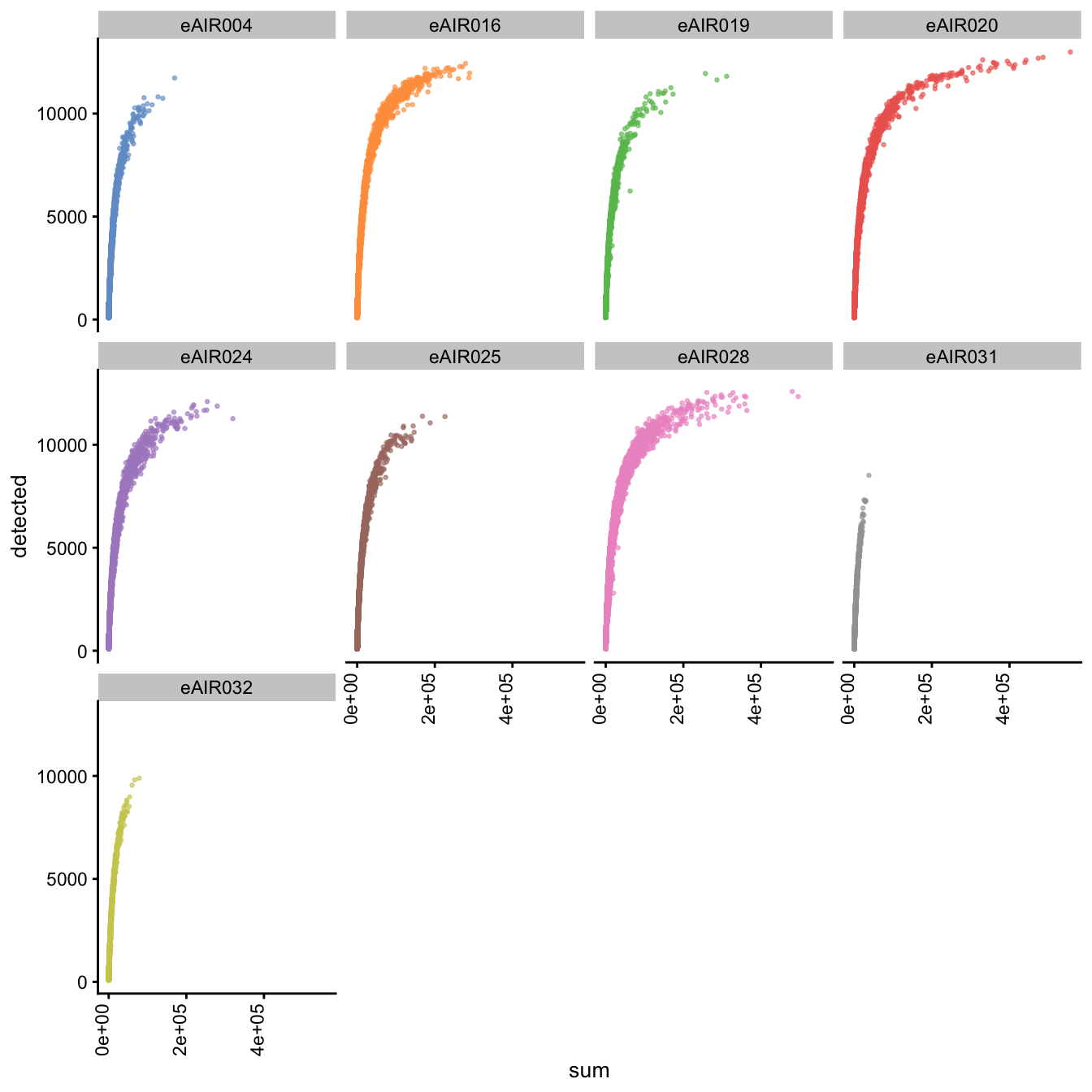
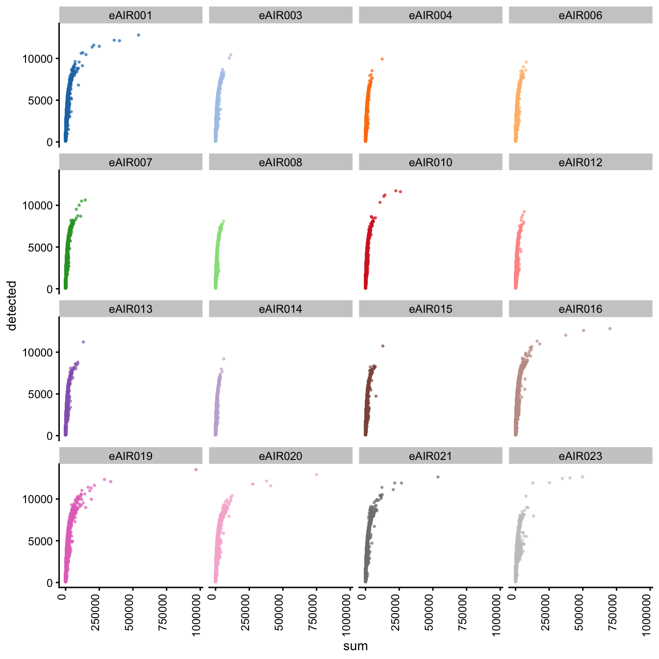
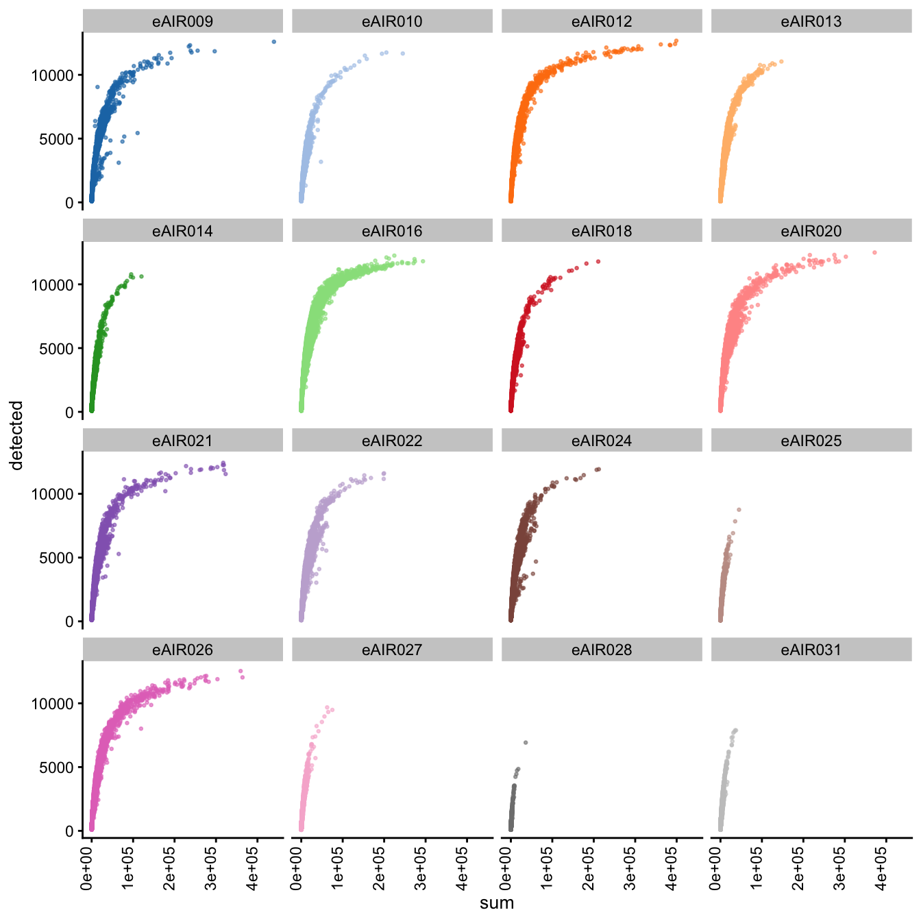
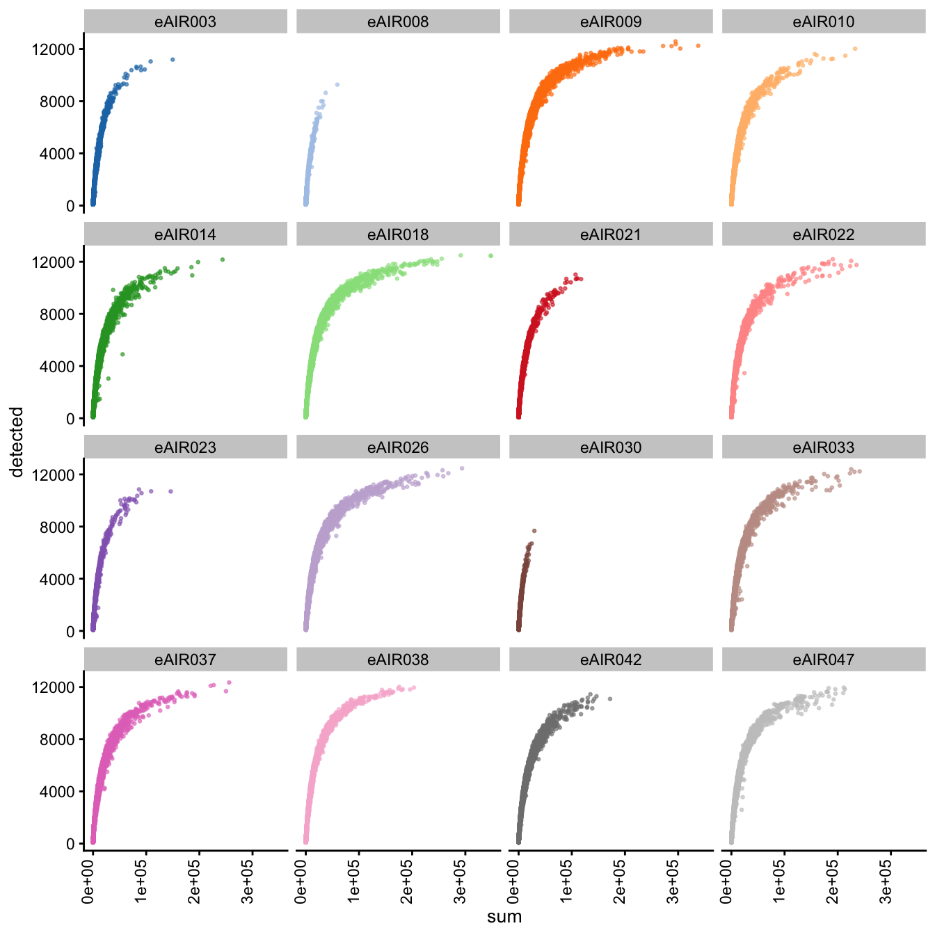
Next, we generate scatter plots depicting the relationship between gene counts (detected) and read counts (sum) for each sample within different batches. The x-axis represents the total read counts, which provide an indication of library size, while the y-axis represents the number of genes detected. This plot helps us understand how gene detection varies with different library sizes across samples within each batch.
for (i in seq_along(batches)){
  batch_name <- batches[i]
  tissue_type <- tissue_types[i]
  cat('### ', batch_name, " - ", tissue_type, '\n')
  sce <- all_sce[[i]]
  p1 <- plotColData(
  sce,
  "detected",
  x = "sum",
  other_fields = "Sample",
  colour_by = "Sample",
  point_size = 0.5) +
  facet_wrap(vars(Sample), ncol = 4) +
  theme(legend.position = "none",
        axis.text.x = element_text(angle = 90, hjust = 1, vjust = 0))

  print(p1)
  cat('\n\n')
}
G000231_Neeland_batch1 - Nasal_brushings
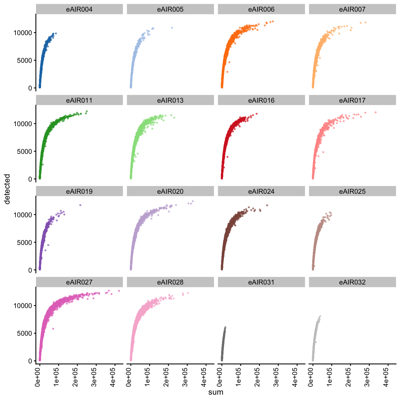
Scatter plot of total counts vs detected
G000231_Neeland_batch2_1 - Tonsils
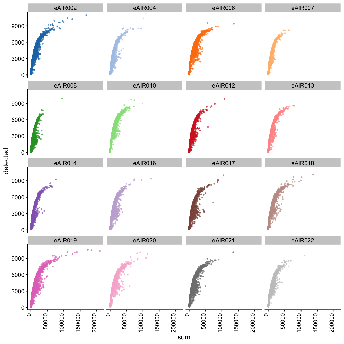
Scatter plot of total counts vs detected
G000231_Neeland_batch2_2 - Nasal_brushings_repeat
Scatter plot of total counts vs detected
G000231_Neeland_batch3 - Adenoids
Scatter plot of total counts vs detected
G000231_Neeland_batch4 - Bronchial_brushings
Scatter plot of total counts vs detected
G000231_Neeland_batch5 - Nasal_brushings_2
Scatter plot of total counts vs detected
Visualize cells with zero counts
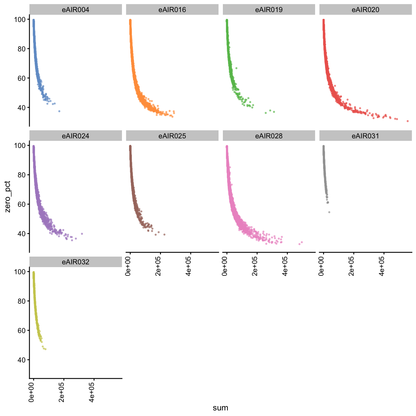
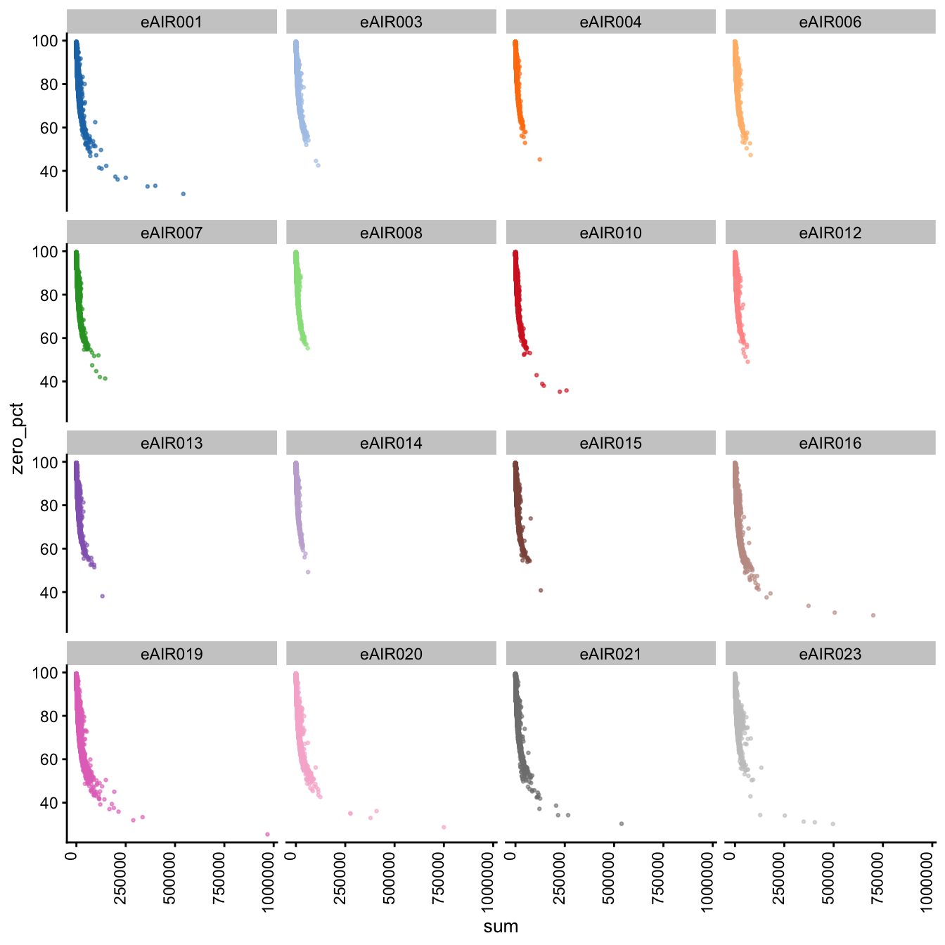
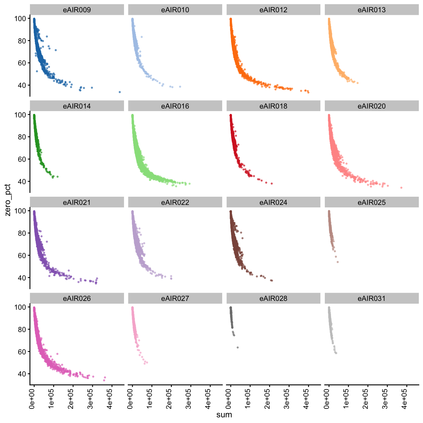
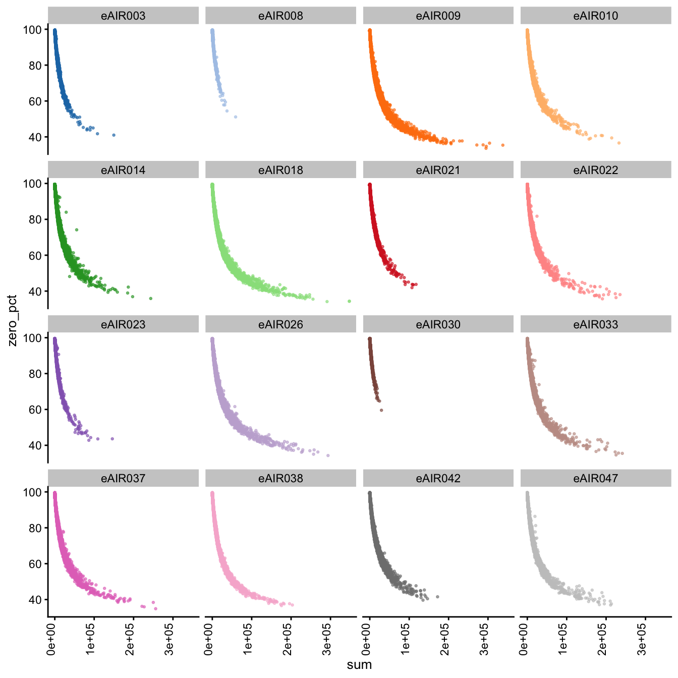
Furthermore, we generate Scatter plots to examine the relationship between the percentage of zeroes in cells (zero_pct) and the total read counts (sum) in each batch. These scatter plots help assess how the proportion of non-expressed cells (zeroes) correlates with the overall expression level (total counts) within different samples of each batch.
These plots can offer insights into whether low total counts are associated with a higher proportion of zero-expression cells, which could indicate potential issues in the data quality.
for (i in seq_along(batches)){
  batch_name <- batches[i]
  tissue_type <- tissue_types[i]
  cat('### ', batch_name, " - ", tissue_type, '\n')
  sce <- all_sce[[i]]
  p1 <- plotColData(
  sce,
  "zero_pct",
  x = "sum",
  other_fields = "Sample",
  colour_by = "Sample",
  point_size = 0.5) +
  facet_wrap(vars(Sample), ncol = 4) +
  theme(legend.position = "none",
        axis.text.x = element_text(angle = 90, hjust = 1, vjust = 0))
  print(p1)
  cat('\n\n')
}
G000231_Neeland_batch1 - Nasal_brushings
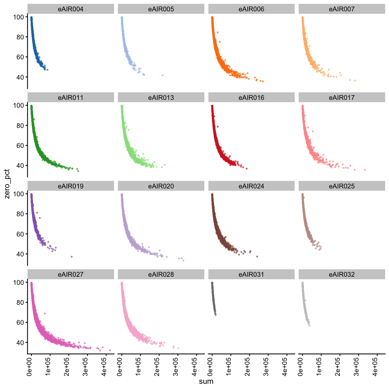
Scatter Plots of Percentage of Zeroes vs Total Counts
G000231_Neeland_batch2_1 - Tonsils
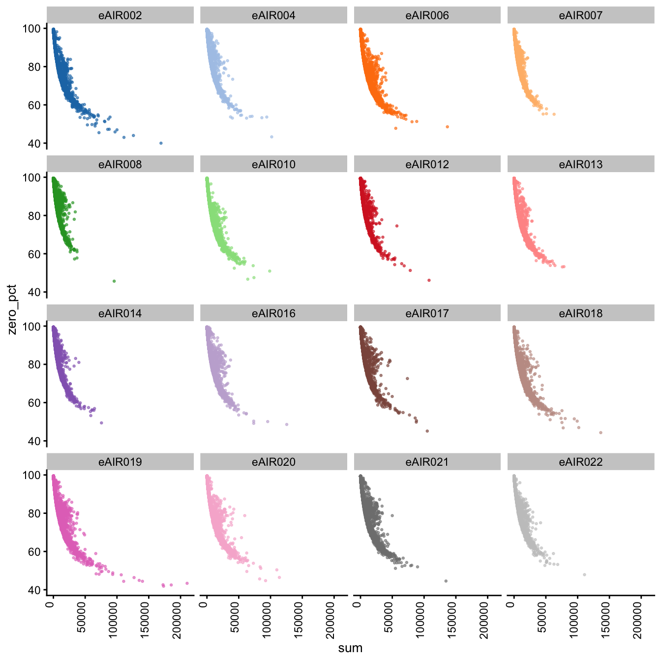
Scatter Plots of Percentage of Zeroes vs Total Counts
G000231_Neeland_batch2_2 - Nasal_brushings_repeat
Scatter Plots of Percentage of Zeroes vs Total Counts
G000231_Neeland_batch3 - Adenoids
Scatter Plots of Percentage of Zeroes vs Total Counts
G000231_Neeland_batch4 - Bronchial_brushings
Scatter Plots of Percentage of Zeroes vs Total Counts
G000231_Neeland_batch5 - Nasal_brushings_2
Scatter Plots of Percentage of Zeroes vs Total Counts
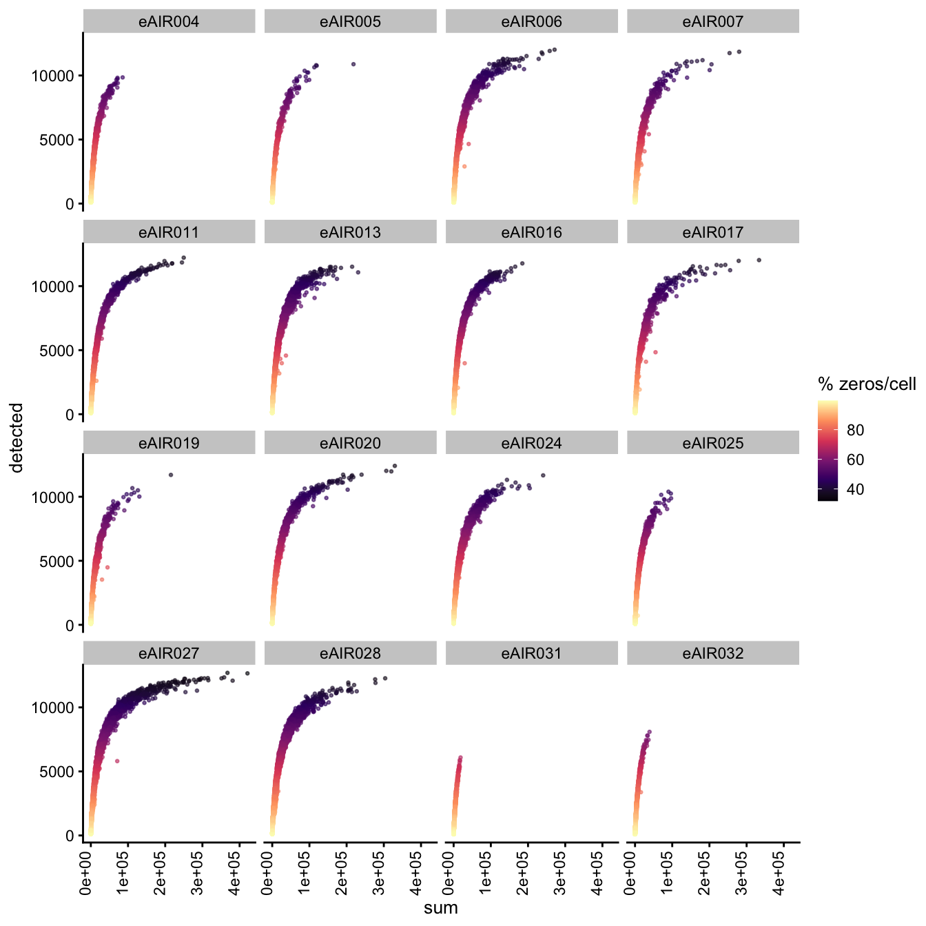
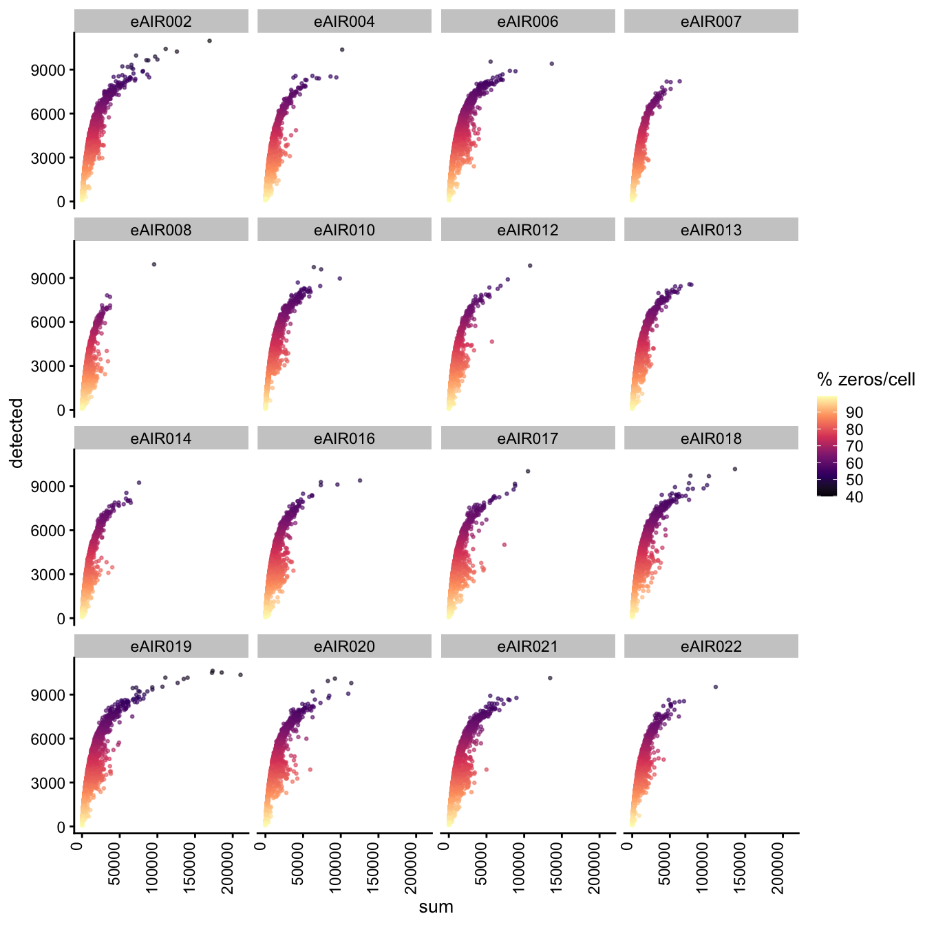
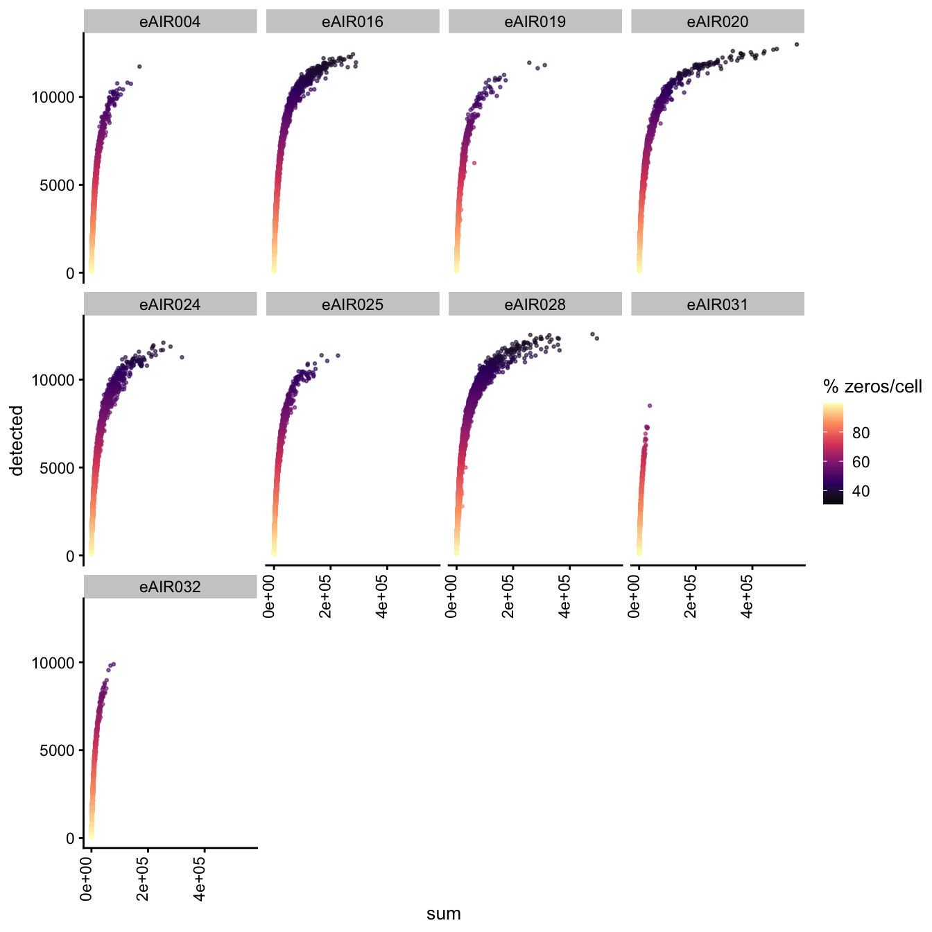
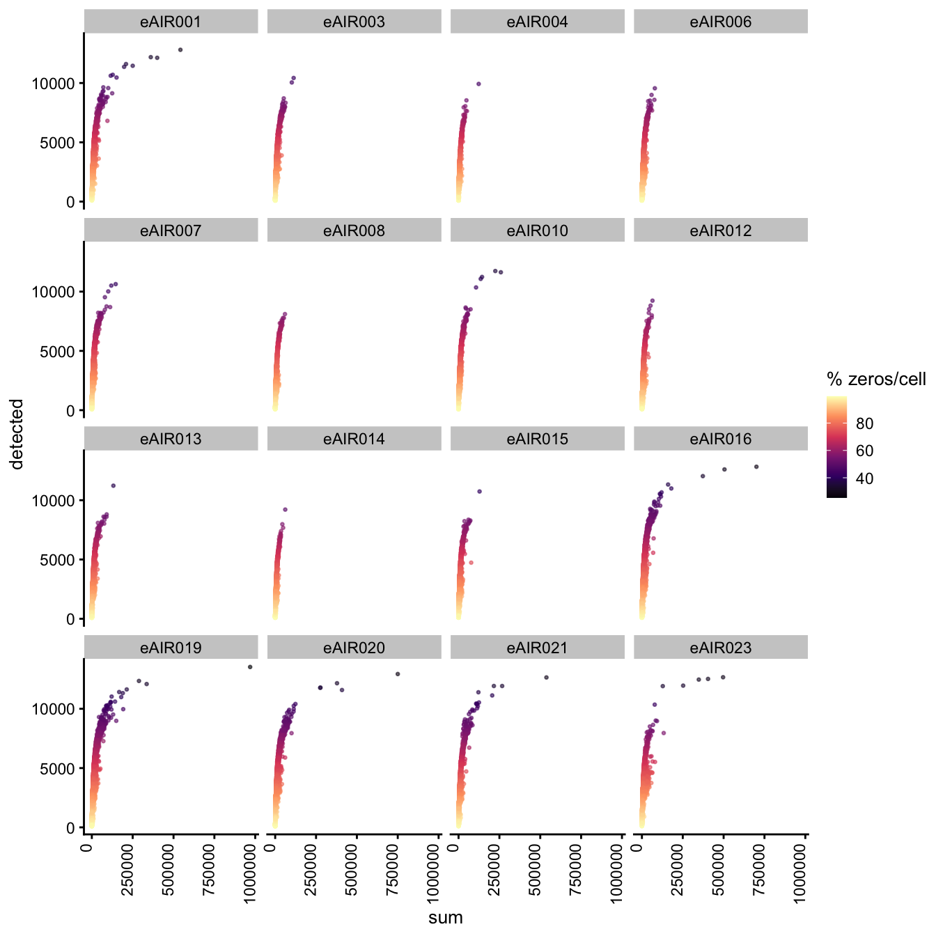
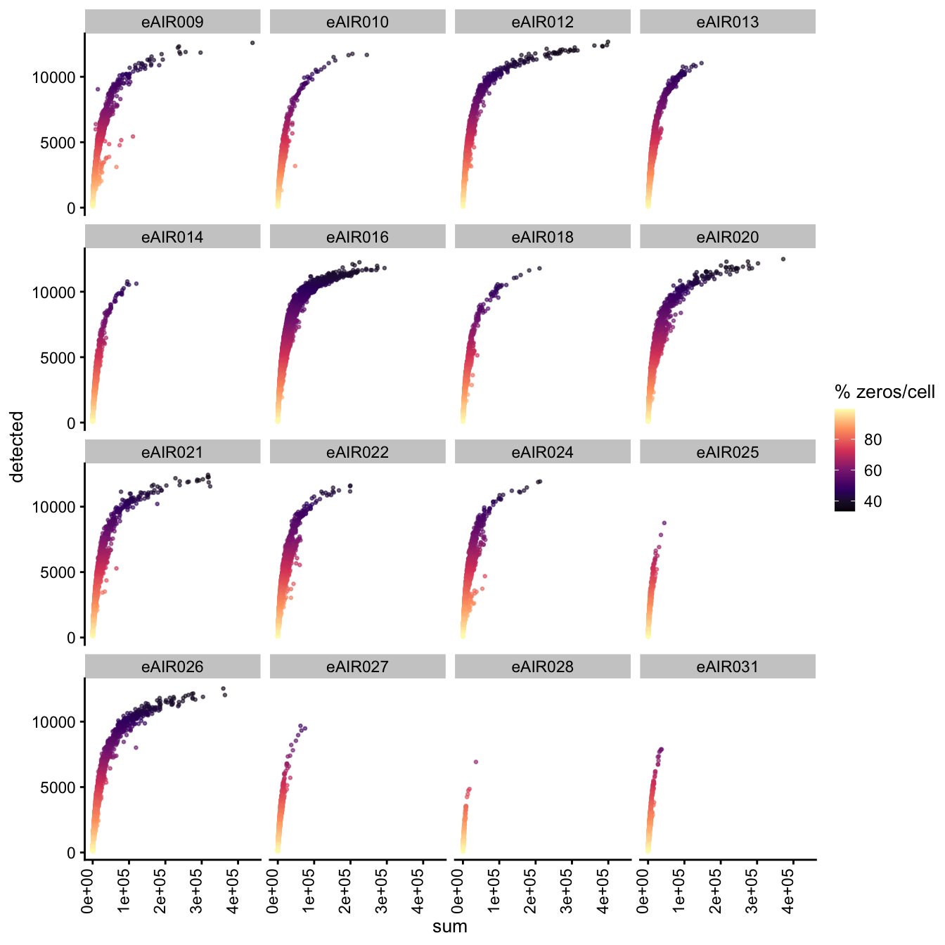
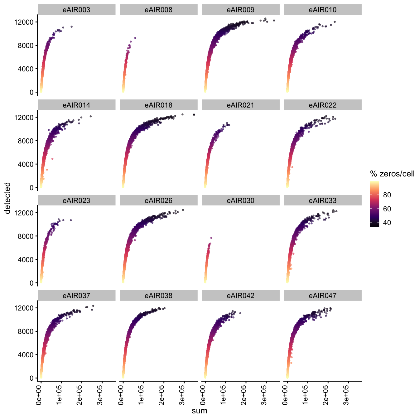
Visualize Percentage of zeroes per cell
Exploring the relationship between detected and sum, color-coded by Percentage of Zero Counts.
for (i in seq_along(batches)){
  batch_name <- batches[i]
  tissue_type <- tissue_types[i]
  cat('### ', batch_name, " - ", tissue_type, '\n')
  sce <- all_sce[[i]]
  p1 <- plotColData(
  sce,
  "detected",
  x = "sum",
  other_fields = "Sample",
  colour_by = "zero_pct",
  point_size = 0.5) +
  facet_wrap(vars(Sample), ncol = 4) +
  theme(axis.text.x = element_text(angle = 90, hjust = 1, vjust = 0)) +
  scale_color_viridis_c(option = "magma") +
  labs(colour = "% zeros/cell")
  print(p1)
  cat('\n\n')
}
G000231_Neeland_batch1 - Nasal_brushings
G000231_Neeland_batch2_1 - Tonsils
G000231_Neeland_batch2_2 - Nasal_brushings_repeat
G000231_Neeland_batch3 - Adenoids
G000231_Neeland_batch4 - Bronchial_brushings
G000231_Neeland_batch5 - Nasal_brushings_2
Session Info
sessionInfo()R version 4.3.1 (2023-06-16)
Platform: x86_64-apple-darwin20 (64-bit)
Running under: macOS Ventura 13.5
Matrix products: default
BLAS: /Library/Frameworks/R.framework/Versions/4.3-x86_64/Resources/lib/libRblas.0.dylib
LAPACK: /Library/Frameworks/R.framework/Versions/4.3-x86_64/Resources/lib/libRlapack.dylib; LAPACK version 3.11.0
locale:
[1] en_AU.UTF-8/en_AU.UTF-8/en_AU.UTF-8/C/en_AU.UTF-8/en_AU.UTF-8
time zone: Australia/Melbourne
tzcode source: internal
attached base packages:
[1] stats4 stats graphics grDevices utils datasets methods
[8] base
other attached packages:
[1] EnsDb.Hsapiens.v86_2.99.0
[2] ensembldb_2.24.0
[3] AnnotationFilter_1.24.0
[4] msigdbr_7.5.1
[5] Homo.sapiens_1.3.1
[6] TxDb.Hsapiens.UCSC.hg19.knownGene_3.2.2
[7] org.Hs.eg.db_3.17.0
[8] GO.db_3.17.0
[9] OrganismDbi_1.42.0
[10] GenomicFeatures_1.52.1
[11] AnnotationDbi_1.62.2
[12] scales_1.2.1
[13] patchwork_1.1.2
[14] cowplot_1.1.1
[15] janitor_2.2.0
[16] scater_1.28.0
[17] scran_1.28.1
[18] scuttle_1.10.1
[19] SingleCellExperiment_1.22.0
[20] SummarizedExperiment_1.30.2
[21] Biobase_2.60.0
[22] GenomicRanges_1.52.0
[23] GenomeInfoDb_1.36.1
[24] IRanges_2.34.1
[25] S4Vectors_0.38.1
[26] BiocGenerics_0.46.0
[27] MatrixGenerics_1.12.2
[28] matrixStats_1.0.0
[29] RColorBrewer_1.1-3
[30] glue_1.6.2
[31] here_1.0.1
[32] lubridate_1.9.2
[33] forcats_1.0.0
[34] stringr_1.5.0
[35] dplyr_1.1.2
[36] purrr_1.0.1
[37] readr_2.1.4
[38] tidyr_1.3.0
[39] tibble_3.2.1
[40] ggplot2_3.4.2
[41] tidyverse_2.0.0
[42] BiocStyle_2.28.0
[43] workflowr_1.7.0
loaded via a namespace (and not attached):
[1] later_1.3.1 BiocIO_1.10.0
[3] bitops_1.0-7 filelock_1.0.2
[5] graph_1.78.0 XML_3.99-0.14
[7] lifecycle_1.0.3 edgeR_3.42.4
[9] rprojroot_2.0.3 processx_3.8.2
[11] lattice_0.21-8 magrittr_2.0.3
[13] limma_3.56.2 sass_0.4.7
[15] rmarkdown_2.23 jquerylib_0.1.4
[17] yaml_2.3.7 metapod_1.8.0
[19] httpuv_1.6.11 DBI_1.1.3
[21] zlibbioc_1.46.0 RCurl_1.98-1.12
[23] rappdirs_0.3.3 git2r_0.32.0
[25] GenomeInfoDbData_1.2.10 ggrepel_0.9.3
[27] irlba_2.3.5.1 dqrng_0.3.0
[29] DelayedMatrixStats_1.22.1 codetools_0.2-19
[31] DelayedArray_0.26.6 xml2_1.3.5
[33] tidyselect_1.2.0 farver_2.1.1
[35] ScaledMatrix_1.8.1 viridis_0.6.4
[37] BiocFileCache_2.8.0 GenomicAlignments_1.36.0
[39] jsonlite_1.8.7 BiocNeighbors_1.18.0
[41] tools_4.3.1 progress_1.2.2
[43] Rcpp_1.0.11 gridExtra_2.3
[45] xfun_0.39 withr_2.5.0
[47] BiocManager_1.30.21.1 fastmap_1.1.1
[49] bluster_1.10.0 fansi_1.0.4
[51] callr_3.7.3 digest_0.6.33
[53] rsvd_1.0.5 timechange_0.2.0
[55] R6_2.5.1 colorspace_2.1-0
[57] biomaRt_2.56.1 RSQLite_2.3.1
[59] utf8_1.2.3 generics_0.1.3
[61] rtracklayer_1.60.0 prettyunits_1.1.1
[63] httr_1.4.6 S4Arrays_1.0.4
[65] whisker_0.4.1 pkgconfig_2.0.3
[67] gtable_0.3.3 blob_1.2.4
[69] XVector_0.40.0 htmltools_0.5.5
[71] RBGL_1.76.0 ProtGenerics_1.32.0
[73] png_0.1-8 snakecase_0.11.0
[75] knitr_1.43 rstudioapi_0.15.0
[77] tzdb_0.4.0 rjson_0.2.21
[79] curl_5.0.1 cachem_1.0.8
[81] parallel_4.3.1 vipor_0.4.5
[83] restfulr_0.0.15 pillar_1.9.0
[85] grid_4.3.1 vctrs_0.6.3
[87] promises_1.2.0.1 BiocSingular_1.16.0
[89] dbplyr_2.3.3 beachmat_2.16.0
[91] cluster_2.1.4 beeswarm_0.4.0
[93] evaluate_0.21 cli_3.6.1
[95] locfit_1.5-9.8 compiler_4.3.1
[97] Rsamtools_2.16.0 rlang_1.1.1
[99] crayon_1.5.2 labeling_0.4.2
[101] ps_1.7.5 getPass_0.2-2
[103] fs_1.6.3 ggbeeswarm_0.7.2
[105] stringi_1.7.12 viridisLite_0.4.2
[107] BiocParallel_1.34.2 babelgene_22.9
[109] munsell_0.5.0 Biostrings_2.68.1
[111] lazyeval_0.2.2 Matrix_1.6-0
[113] hms_1.1.3 sparseMatrixStats_1.12.2
[115] bit64_4.0.5 KEGGREST_1.40.0
[117] statmod_1.5.0 highr_0.10
[119] igraph_1.5.0 memoise_2.0.1
[121] bslib_0.5.0 bit_4.0.5