Adenoids
Clustering and Marker gene analysis
Gunjan Dixit
July 26, 2024
Last updated: 2024-07-26
Checks: 6 1
Knit directory: paed-airway-allTissues/
This reproducible R Markdown analysis was created with workflowr (version 1.7.1). The Checks tab describes the reproducibility checks that were applied when the results were created. The Past versions tab lists the development history.
The R Markdown file has unstaged changes. To know which version of
the R Markdown file created these results, you’ll want to first commit
it to the Git repo. If you’re still working on the analysis, you can
ignore this warning. When you’re finished, you can run
wflow_publish to commit the R Markdown file and build the
HTML.
Great job! The global environment was empty. Objects defined in the global environment can affect the analysis in your R Markdown file in unknown ways. For reproduciblity it’s best to always run the code in an empty environment.
The command set.seed(20230811) was run prior to running
the code in the R Markdown file. Setting a seed ensures that any results
that rely on randomness, e.g. subsampling or permutations, are
reproducible.
Great job! Recording the operating system, R version, and package versions is critical for reproducibility.
Nice! There were no cached chunks for this analysis, so you can be confident that you successfully produced the results during this run.
Great job! Using relative paths to the files within your workflowr project makes it easier to run your code on other machines.
Great! You are using Git for version control. Tracking code development and connecting the code version to the results is critical for reproducibility.
The results in this page were generated with repository version 649de68. See the Past versions tab to see a history of the changes made to the R Markdown and HTML files.
Note that you need to be careful to ensure that all relevant files for
the analysis have been committed to Git prior to generating the results
(you can use wflow_publish or
wflow_git_commit). workflowr only checks the R Markdown
file, but you know if there are other scripts or data files that it
depends on. Below is the status of the Git repository when the results
were generated:
Ignored files:
    Ignored:    .DS_Store
    Ignored:    .RData
    Ignored:    .Rhistory
    Ignored:    .Rproj.user/
    Ignored:    analysis/.DS_Store
    Ignored:    data/.DS_Store
    Ignored:    data/RDS/
    Ignored:    output/.DS_Store
    Ignored:    output/CSV/.DS_Store
    Ignored:    output/G000231_Neeland_batch1/
    Ignored:    output/G000231_Neeland_batch2_1/
    Ignored:    output/G000231_Neeland_batch2_2/
    Ignored:    output/G000231_Neeland_batch3/
    Ignored:    output/G000231_Neeland_batch4/
    Ignored:    output/G000231_Neeland_batch5/
    Ignored:    output/G000231_Neeland_batch9_1/
    Ignored:    output/RDS/
    Ignored:    output/plots/

Untracked files:
    Untracked:  VennDiagram.2024-07-24_11-48-08.297746.log
    Untracked:  VennDiagram.2024-07-24_12-25-12.854839.log
    Untracked:  VennDiagram.2024-07-24_12-25-22.005094.log
    Untracked:  VennDiagram.2024-07-24_12-29-34.757841.log
    Untracked:  analysis/03_Batch_Integration.Rmd
    Untracked:  analysis/Age_proportions.Rmd
    Untracked:  analysis/Age_proportions_AllBatches.Rmd
    Untracked:  analysis/Batch_Integration_&_Downstream_analysis.Rmd
    Untracked:  analysis/Batch_correction_&_Downstream.Rmd
    Untracked:  analysis/Cell_cycle_regression.Rmd
    Untracked:  analysis/Preprocessing_Batch1_Nasal_brushings.Rmd
    Untracked:  analysis/Preprocessing_Batch2_Tonsils.Rmd
    Untracked:  analysis/Preprocessing_Batch3_Adenoids.Rmd
    Untracked:  analysis/Preprocessing_Batch4_Bronchial_brushings.Rmd
    Untracked:  analysis/Preprocessing_Batch5_Nasal_brushings.Rmd
    Untracked:  analysis/Preprocessing_Batch6_BAL.Rmd
    Untracked:  analysis/Preprocessing_Batch7_Bronchial_brushings.Rmd
    Untracked:  analysis/Preprocessing_Batch8_Adenoids.Rmd
    Untracked:  analysis/Preprocessing_Batch9_Tonsils.Rmd
    Untracked:  analysis/VennDiagram.2024-07-24_11-54-23.569848.log
    Untracked:  analysis/VennDiagram.2024-07-24_11-55-06.582353.log
    Untracked:  analysis/VennDiagram.2024-07-24_12-28-47.017253.log
    Untracked:  analysis/VennDiagram.2024-07-24_12-33-05.913419.log
    Untracked:  analysis/VennDiagram.2024-07-24_13-42-31.593316.log
    Untracked:  analysis/cell_cycle_regression.R
    Untracked:  analysis/test.Rmd
    Untracked:  analysis/testing_age_all.Rmd
    Untracked:  data/Cell_labels_Mel/
    Untracked:  data/Cell_labels_Mel_v2/
    Untracked:  data/Hs.c2.cp.reactome.v7.1.entrez.rds
    Untracked:  data/Raw_feature_bc_matrix/
    Untracked:  data/celltypes_Mel_GD_v3.xlsx
    Untracked:  data/celltypes_Mel_GD_v4_no_dups.xlsx
    Untracked:  data/celltypes_Mel_modified.xlsx
    Untracked:  data/celltypes_Mel_v2.csv
    Untracked:  data/celltypes_Mel_v2.xlsx
    Untracked:  data/celltypes_Mel_v2_MN.xlsx
    Untracked:  data/celltypes_for_mel_MN.xlsx
    Untracked:  data/earlyAIR_sample_sheets_combined.xlsx
    Untracked:  output/CSV/Bronchial_brushings_Marker_gene_clusters.limmaTrendRNA_snn_res.0.4/
    Untracked:  stacked_barplot.png
    Untracked:  stacked_barplot_donor_id.png

Unstaged changes:
    Deleted:    02_QC_exploratoryPlots.Rmd
    Deleted:    02_QC_exploratoryPlots.html
    Modified:   analysis/00_AllBatches_overview.Rmd
    Modified:   analysis/01_QC_emptyDrops.Rmd
    Modified:   analysis/02_QC_exploratoryPlots.Rmd
    Modified:   analysis/Adenoids.Rmd
    Modified:   analysis/Age_modeling.Rmd
    Modified:   analysis/AllBatches_QCExploratory.Rmd
    Modified:   analysis/BAL.Rmd
    Modified:   analysis/Bronchial_brushings.Rmd
    Modified:   analysis/Tonsils.Rmd
    Modified:   output/CSV/BAL_Marker_gene_clusters.limmaTrendRNA_snn_res.0.4/REACTOME-cluster-limma-c0.csv
    Modified:   output/CSV/BAL_Marker_gene_clusters.limmaTrendRNA_snn_res.0.4/REACTOME-cluster-limma-c1.csv
    Modified:   output/CSV/BAL_Marker_gene_clusters.limmaTrendRNA_snn_res.0.4/REACTOME-cluster-limma-c10.csv
    Modified:   output/CSV/BAL_Marker_gene_clusters.limmaTrendRNA_snn_res.0.4/REACTOME-cluster-limma-c11.csv
    Modified:   output/CSV/BAL_Marker_gene_clusters.limmaTrendRNA_snn_res.0.4/REACTOME-cluster-limma-c12.csv
    Modified:   output/CSV/BAL_Marker_gene_clusters.limmaTrendRNA_snn_res.0.4/REACTOME-cluster-limma-c13.csv
    Modified:   output/CSV/BAL_Marker_gene_clusters.limmaTrendRNA_snn_res.0.4/REACTOME-cluster-limma-c14.csv
    Modified:   output/CSV/BAL_Marker_gene_clusters.limmaTrendRNA_snn_res.0.4/REACTOME-cluster-limma-c15.csv
    Modified:   output/CSV/BAL_Marker_gene_clusters.limmaTrendRNA_snn_res.0.4/REACTOME-cluster-limma-c16.csv
    Modified:   output/CSV/BAL_Marker_gene_clusters.limmaTrendRNA_snn_res.0.4/REACTOME-cluster-limma-c17.csv
    Modified:   output/CSV/BAL_Marker_gene_clusters.limmaTrendRNA_snn_res.0.4/REACTOME-cluster-limma-c2.csv
    Modified:   output/CSV/BAL_Marker_gene_clusters.limmaTrendRNA_snn_res.0.4/REACTOME-cluster-limma-c3.csv
    Modified:   output/CSV/BAL_Marker_gene_clusters.limmaTrendRNA_snn_res.0.4/REACTOME-cluster-limma-c4.csv
    Modified:   output/CSV/BAL_Marker_gene_clusters.limmaTrendRNA_snn_res.0.4/REACTOME-cluster-limma-c5.csv
    Modified:   output/CSV/BAL_Marker_gene_clusters.limmaTrendRNA_snn_res.0.4/REACTOME-cluster-limma-c6.csv
    Modified:   output/CSV/BAL_Marker_gene_clusters.limmaTrendRNA_snn_res.0.4/REACTOME-cluster-limma-c7.csv
    Modified:   output/CSV/BAL_Marker_gene_clusters.limmaTrendRNA_snn_res.0.4/REACTOME-cluster-limma-c8.csv
    Modified:   output/CSV/BAL_Marker_gene_clusters.limmaTrendRNA_snn_res.0.4/REACTOME-cluster-limma-c9.csv
    Modified:   output/CSV/BAL_Marker_gene_clusters.limmaTrendRNA_snn_res.0.4/up-cluster-limma-c0.csv
    Modified:   output/CSV/BAL_Marker_gene_clusters.limmaTrendRNA_snn_res.0.4/up-cluster-limma-c1.csv
    Modified:   output/CSV/BAL_Marker_gene_clusters.limmaTrendRNA_snn_res.0.4/up-cluster-limma-c10.csv
    Modified:   output/CSV/BAL_Marker_gene_clusters.limmaTrendRNA_snn_res.0.4/up-cluster-limma-c11.csv
    Modified:   output/CSV/BAL_Marker_gene_clusters.limmaTrendRNA_snn_res.0.4/up-cluster-limma-c12.csv
    Modified:   output/CSV/BAL_Marker_gene_clusters.limmaTrendRNA_snn_res.0.4/up-cluster-limma-c13.csv
    Modified:   output/CSV/BAL_Marker_gene_clusters.limmaTrendRNA_snn_res.0.4/up-cluster-limma-c14.csv
    Modified:   output/CSV/BAL_Marker_gene_clusters.limmaTrendRNA_snn_res.0.4/up-cluster-limma-c15.csv
    Modified:   output/CSV/BAL_Marker_gene_clusters.limmaTrendRNA_snn_res.0.4/up-cluster-limma-c16.csv
    Modified:   output/CSV/BAL_Marker_gene_clusters.limmaTrendRNA_snn_res.0.4/up-cluster-limma-c17.csv
    Modified:   output/CSV/BAL_Marker_gene_clusters.limmaTrendRNA_snn_res.0.4/up-cluster-limma-c2.csv
    Modified:   output/CSV/BAL_Marker_gene_clusters.limmaTrendRNA_snn_res.0.4/up-cluster-limma-c3.csv
    Modified:   output/CSV/BAL_Marker_gene_clusters.limmaTrendRNA_snn_res.0.4/up-cluster-limma-c4.csv
    Modified:   output/CSV/BAL_Marker_gene_clusters.limmaTrendRNA_snn_res.0.4/up-cluster-limma-c5.csv
    Modified:   output/CSV/BAL_Marker_gene_clusters.limmaTrendRNA_snn_res.0.4/up-cluster-limma-c6.csv
    Modified:   output/CSV/BAL_Marker_gene_clusters.limmaTrendRNA_snn_res.0.4/up-cluster-limma-c7.csv
    Modified:   output/CSV/BAL_Marker_gene_clusters.limmaTrendRNA_snn_res.0.4/up-cluster-limma-c8.csv
    Modified:   output/CSV/BAL_Marker_gene_clusters.limmaTrendRNA_snn_res.0.4/up-cluster-limma-c9.csv
Note that any generated files, e.g. HTML, png, CSS, etc., are not included in this status report because it is ok for generated content to have uncommitted changes.
These are the previous versions of the repository in which changes were
made to the R Markdown (analysis/Adenoids.Rmd) and HTML
(docs/Adenoids.html) files. If you’ve configured a remote
Git repository (see ?wflow_git_remote), click on the
hyperlinks in the table below to view the files as they were in that
past version.
| File | Version | Author | Date | Message |
|---|---|---|---|---|
| Rmd | 649de68 | Gunjan Dixit | 2024-07-19 | Added corresponding Azimuth reference plots |
| html | 649de68 | Gunjan Dixit | 2024-07-19 | Added corresponding Azimuth reference plots |
| Rmd | 8b388e7 | Gunjan Dixit | 2024-07-17 | Updated Adenoid/Tonsils Tcell & GC reclustering |
| html | 8b388e7 | Gunjan Dixit | 2024-07-17 | Updated Adenoid/Tonsils Tcell & GC reclustering |
| Rmd | c20f60f | Gunjan Dixit | 2024-07-08 | Updated marker gene dot plots |
| html | c20f60f | Gunjan Dixit | 2024-07-08 | Updated marker gene dot plots |
| Rmd | 77c742e | Gunjan Dixit | 2024-06-26 | Updated RMarkdown files of all Tissues |
| html | 77c742e | Gunjan Dixit | 2024-06-26 | Updated RMarkdown files of all Tissues |
| Rmd | f27efbf | Gunjan Dixit | 2024-06-25 | Updated reclustering of Tonsils/Adenoids |
| html | f27efbf | Gunjan Dixit | 2024-06-25 | Updated reclustering of Tonsils/Adenoids |
| html | a94371e | Gunjan Dixit | 2024-06-07 | Reclustering analysis |
| Rmd | e0e83af | Gunjan Dixit | 2024-06-04 | Updated reclustering |
| Rmd | 5aee5dd | Gunjan Dixit | 2024-05-07 | Modified Adenoids/Tonsils analysis |
| html | 5aee5dd | Gunjan Dixit | 2024-05-07 | Modified Adenoids/Tonsils analysis |
| Rmd | 320ccbd | Gunjan Dixit | 2024-05-01 | Modified/Annotated RMarkdown files |
| html | 320ccbd | Gunjan Dixit | 2024-05-01 | Modified/Annotated RMarkdown files |
| Rmd | 9492583 | Gunjan Dixit | 2024-04-26 | Added new analysis |
| html | 9492583 | Gunjan Dixit | 2024-04-26 | Added new analysis |
Introduction
This Rmarkdown file loads and analyzes the batch-integrated/merged
Seurat object for Adenoids (Batch3 and Batch8). It
performs clustering at various resolutions ranging from 0-1, followed by
visualization of identified clusters and Broad Level 3 cell labels on
UMAP. Next, the FindAllMarkers function is used to perform
marker gene analysis to identify marker genes for each cluster. The top
marker gene is visualized using FeaturePlot,
ViolinPlot and Heatmap. The identified marker
genes are stored in CSV format for each cluster at the optimum
resolution identified using clustree function.
Load libraries
suppressPackageStartupMessages({
  library(BiocStyle)
  library(tidyverse)
  library(here)
  library(dplyr)
  library(Seurat)
  library(clustree)
  library(kableExtra)
  library(RColorBrewer)
  library(data.table)
  library(ggplot2)
  library(patchwork)
  library(readxl)
})
Load Input data
Load merged object (batch corrected/integrated) for the tissue.
tissue <- "Adenoids"
out <- here("output/RDS/AllBatches_Harmony_SEUs/G000231_Neeland_Adenoids_batchCorrection.Harmony.clusters.SEU.rds")
merged_obj <- readRDS(out)
merged_obj
An object of class Seurat
17456 features across 124956 samples within 1 assay
Active assay: RNA (17456 features, 2000 variable features)
5 layers present: counts.G000231_batch3, counts.G000231_batch8, scale.data, data.G000231_batch3, data.G000231_batch8
4 dimensional reductions calculated: pca, umap.unintegrated, harmony, umap.harmonyClustering
Clustering is done on the “harmony” or batch integrated reduction at resolutions ranging from 0-1.
out1 <- here("output",
            "RDS", "AllBatches_Clustering_SEUs",
             paste0("G000231_Neeland_",tissue,".Clusters.SEU.rds"))
#dir.create(out1)

resolutions <- seq(0.1, 1, by = 0.1)
if (!file.exists(out1)) {
merged_obj <- FindNeighbors(merged_obj, reduction = "harmony", dims = 1:30)
merged_obj <- FindClusters(merged_obj, resolution = seq(0.1, 1, by = 0.1), algorithm = 3)
saveRDS(merged_obj, file = out1)
} else {
    merged_obj <- readRDS(out1)
}
The clustree function is used to visualize the
clustering at different resolutions to identify the most optimum
resolution.
clustree(merged_obj, prefix = "RNA_snn_res.")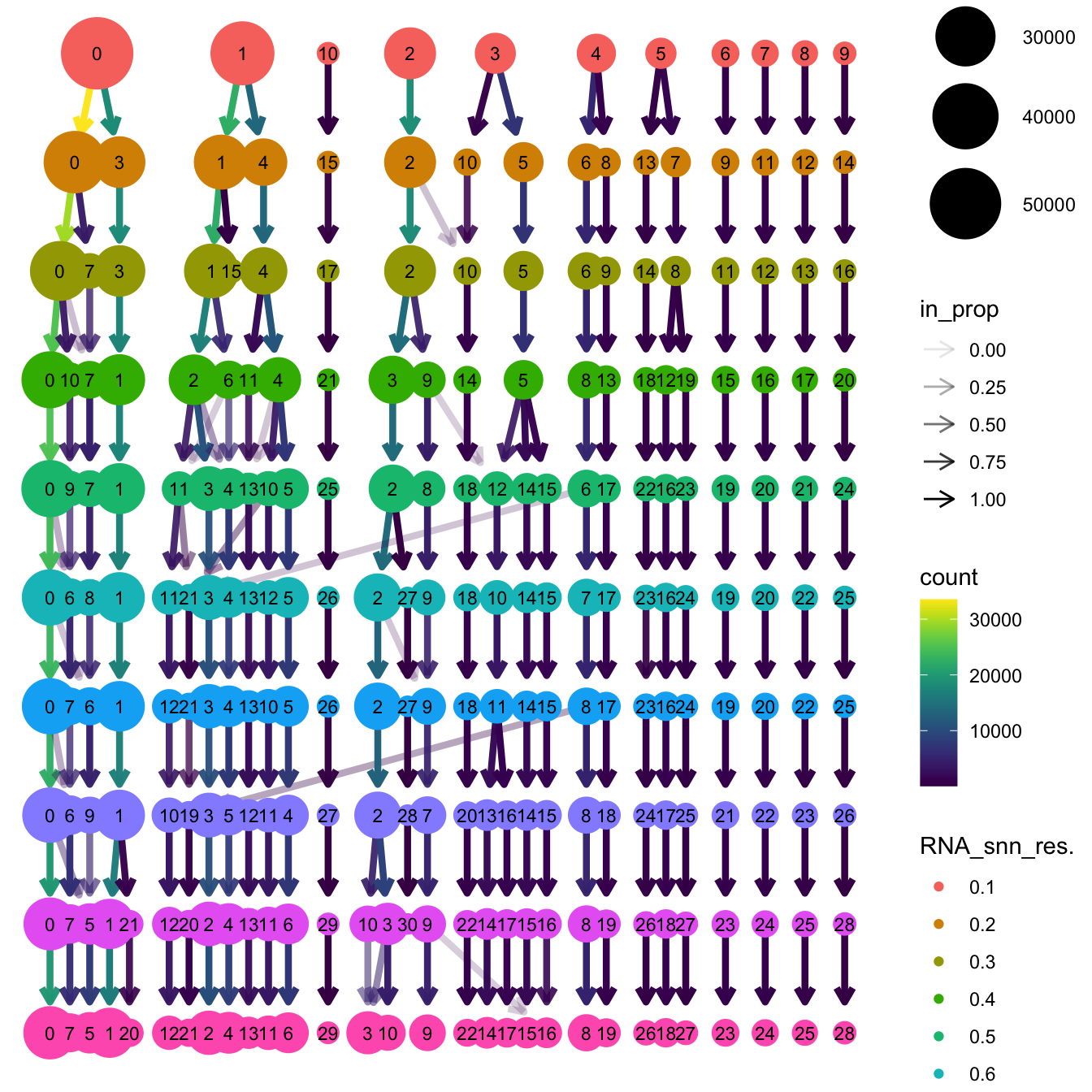
| Version | Author | Date |
|---|---|---|
| 9492583 | Gunjan Dixit | 2024-04-26 |
Based on the clustering tree, we chose an intermediate/optimum resolution where the clustering results are the most stable, with the least amount of shuffling cells.
opt_res <- "RNA_snn_res.0.4"
n <- nlevels(merged_obj$RNA_snn_res.0.4)
merged_obj$RNA_snn_res.0.4 <- factor(merged_obj$RNA_snn_res.0.4, levels = seq(0,n-1))
merged_obj$seurat_clusters <- NULL
merged_obj$cluster <- merged_obj$RNA_snn_res.0.4
Idents(merged_obj) <- merged_obj$cluster
UMAP after clustering
Defining colours for each cell-type to be consistent with other age-related/cell type composition plots.
my_colors <- c(
  "B cells" = "steelblue",
  "CD4 T cells" = "brown",
  "Double negative T cells" = "gold",
  "CD8 T cells" = "lightgreen",
  "Pre B/T cells" = "orchid",
  "Innate lymphoid cells" = "tan",
  "Natural Killer cells" = "blueviolet",
  "Macrophages" = "green4",
  "Cycling T cells" = "turquoise",
  "Dendritic cells" = "grey80",
  "Gamma delta T cells" = "mediumvioletred",
  "Epithelial lineage" = "darkorange",
  "Granulocytes" = "olivedrab",
  "Fibroblast lineage" = "lavender",
  "None" = "white",
  "Monocytes" = "peachpuff",
  "Endothelial lineage" = "cadetblue",
  "SMG duct" = "lightpink",
  "Neuroendocrine" = "skyblue",
  "Doublet query/Other" = "#d62728"
)
# Define custom colors
custom_colors <- list()
colors_1 <- c(
  '#FFC312', '#C4E538', '#12CBC4', '#FDA7DF', '#ED4C67',
  "lavender", '#A3CB38', '#1289A7', '#D980FA', '#B53471',
  '#EE5A24', '#009432', '#0652DD', '#9980FA', '#833471',
  '#EA2027', '#006266', '#1B1464', '#5758BB', '#6F1E51'
)

colors_2 <- c(
  "darkorange", '#cc8e35', '#ffe119', '#4363d8', '#ffda79',
  '#911eb4', '#42d4f4', '#f032e6', '#bfef45', 'grey90',
  '#469990', '#dcbeff', '#9A6324', '#fffac8', '#800000',
  '#aaffc3', '#808000', '#ffd8b1', '#000075', '#a9a9a9'
)

custom_colors$discrete <- c(colors_1, colors_2)
UMAP displaying clusters at opt_res resolution and Broad
cell Labels Level 3.
p1 <- DimPlot(merged_obj, reduction = "umap.harmony", raster = FALSE ,repel = TRUE, label = TRUE,label.size = 3.5, group.by = opt_res) +  NoLegend()

p2 <- DimPlot(merged_obj, reduction = "umap.harmony", raster = FALSE, repel = TRUE, label = TRUE, label.size = 3.5, group.by = "Broad_cell_label_3")  +
  scale_colour_manual(values = my_colors) +
  ggtitle(paste0(tissue, ": Batch Corrected UMAP"))


p1 / p2 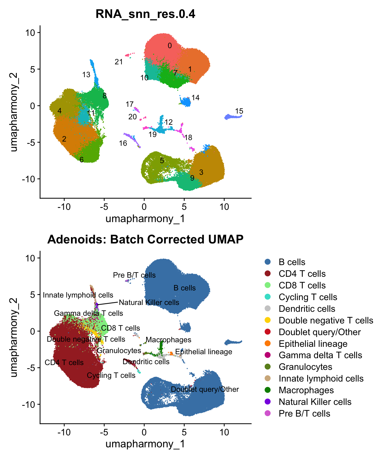
p3 <- DimPlot(merged_obj, reduction = "umap.harmony", raster = FALSE, repel = TRUE, label = TRUE, label.size = 3.5, group.by = "predicted.celltype.l1") + NoLegend()
p3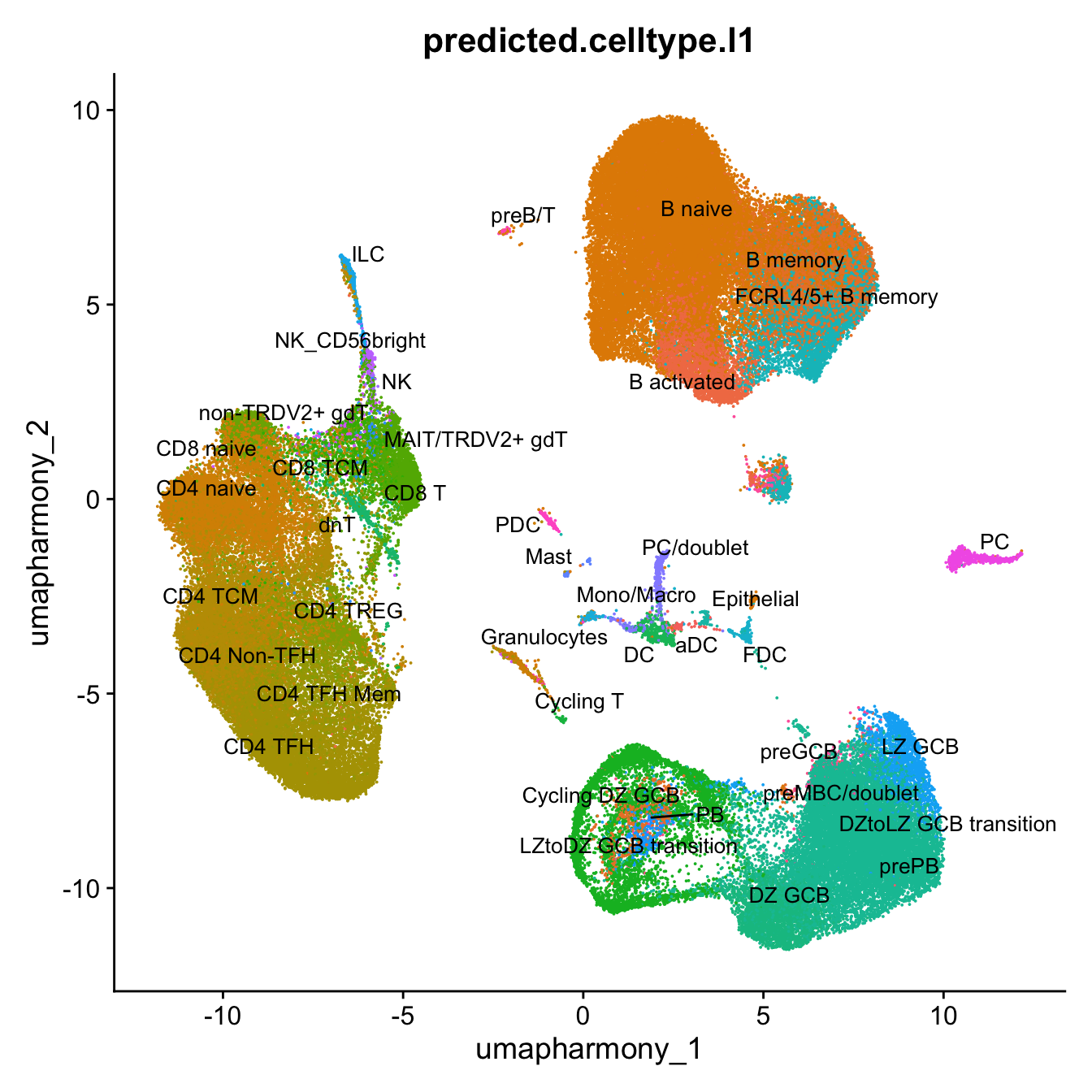
| Version | Author | Date |
|---|---|---|
| 5aee5dd | Gunjan Dixit | 2024-05-07 |
p4 <- DimPlot(merged_obj, reduction = "umap.harmony", raster = FALSE, repel = TRUE, label = TRUE, label.size = 3.5, group.by = "predicted.celltype.l2") + NoLegend()
p4
Warning: ggrepel: 37 unlabeled data points (too many overlaps). Consider
increasing max.overlaps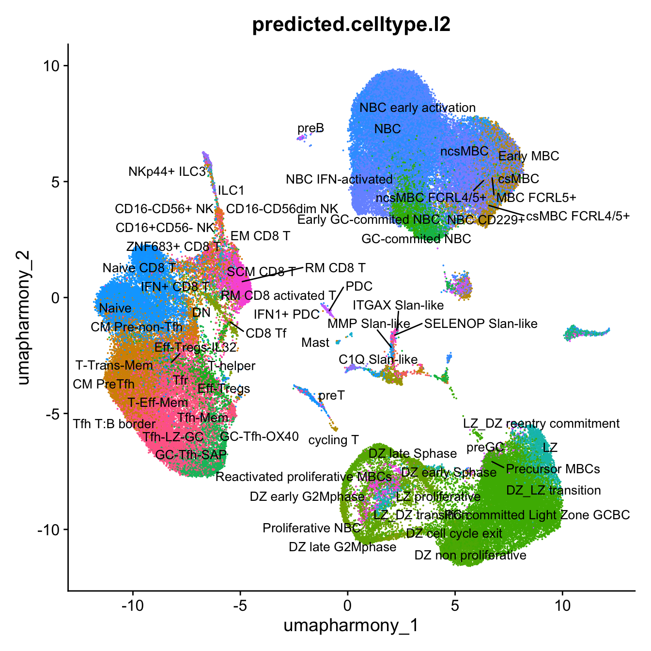
| Version | Author | Date |
|---|---|---|
| 5aee5dd | Gunjan Dixit | 2024-05-07 |
p1 <- merged_obj@meta.data %>%
  ggplot(aes(x = !!sym(opt_res),
             fill = !!sym(opt_res))) +
  geom_bar() +
  geom_text(aes(label = ..count..), stat = "count",
            vjust = -0.5, colour = "black", size = 2) +
  scale_y_log10() +
  theme(axis.text.x = element_text(angle = 90,
                                   vjust = 0.5,
                                   hjust = 1,
                                   size = 8)) +
  NoLegend() +
  labs(y = "No. Cells (log scale)")

p2 <- merged_obj@meta.data %>%
  dplyr::select(!!sym(opt_res), predicted.celltype.l1) %>%
  group_by(!!sym(opt_res), predicted.celltype.l1) %>%
  summarise(num = n()) %>%
  mutate(prop = num / sum(num)) %>%
  ggplot(aes(x = !!sym(opt_res), y = prop * 100,
             fill = predicted.celltype.l1)) +
  geom_bar(stat = "identity") +
  theme(axis.text.x = element_text(angle = 90,
                                   vjust = 0.5,
                                   hjust = 1,
                                   size = 8)) +
  labs(y = "% Cells", fill = "predicted.celltype.l1") +
  scale_fill_manual(values = custom_colors$discrete) #+
`summarise()` has grouped output by 'RNA_snn_res.0.4'. You can override using
the `.groups` argument. # paletteer::scale_fill_paletteer_d("ggsci::default_igv")
p3 <- merged_obj@meta.data %>%
dplyr::select(!!sym(opt_res), Broad_cell_label_3) %>%
group_by(!!sym(opt_res), Broad_cell_label_3) %>%
summarise(num = n()) %>%
mutate(prop = num / sum(num)) %>%
ggplot(aes(x = !!sym(opt_res), y = prop * 100,
fill = Broad_cell_label_3)) +
geom_bar(stat = "identity") +
theme(axis.text.x = element_text(angle = 90,
vjust = 0.5,
hjust = 1,
size = 8)) +
labs(y = "% Cells", fill = "Sample") +
scale_fill_manual(values = my_colors) `summarise()` has grouped output by 'RNA_snn_res.0.4'. You can override using
the `.groups` argument.# Combine the plots
(p1 / p2 / p3 ) & theme(legend.text = element_text(size = 8),
legend.key.size = unit(3, "mm"))
| Version | Author | Date |
|---|---|---|
| 5aee5dd | Gunjan Dixit | 2024-05-07 |
This table shows Azimuth Level 2 predicted cell types and their counts in each cluster in descending order.
cluster_ids <- sort(unique(merged_obj$cluster))
cluster_celltype_counts <- list()

for (cluster_id in cluster_ids) {
  cluster_data <- merged_obj@meta.data[merged_obj$cluster == cluster_id, ]
  table_counts <- table(cluster_data$predicted.celltype.l2)
  sorted_table <- table_counts[order(-table_counts)]
  cluster_celltype_counts[[as.character(cluster_id)]] <- sorted_table
}

cluster_celltype_counts
$`0`
NBC NBC early activation
12713 11574
ncsMBC NBC IFN-activated
517 336
Early GC-commited NBC GC-commited NBC
116 28
Early MBC ncsMBC FCRL4/5+
25 23
csMBC MBC derived early PC precursor
10 4
MBC FCRL5+ CM CD8 T
4 1
$`1`
ncsMBC NBC
4912 3359
ncsMBC FCRL4/5+ csMBC
3095 2680
csMBC FCRL4/5+ NBC early activation
1369 1213
MBC FCRL5+ Early MBC
717 178
NBC IFN-activated Early GC-commited NBC
75 28
GC-commited NBC Precursor MBCs
21 11
NBC CD229+ MBC derived early PC precursor
4 3
DZ_LZ transition preGC
2 2
$`2`
CM PreTfh Tfh-LZ-GC
5467 4773
Tfh-Mem CM Pre-non-Tfh
1852 1363
Eff-Tregs T-Eff-Mem
894 651
Eff-Tregs-IL32 Naive
592 512
T-helper T-Trans-Mem
378 288
GC-Tfh-SAP GC-Tfh-OX40
63 53
Tfr NBC
36 30
Tfh T:B border CM CD8 T
30 28
DN GC-commited NBC
20 12
MAIT/CD161+TRDV2+ gd T-cells SCM CD8 T
10 10
NBC early activation NKp44+ ILC3
9 5
csMBC cycling T
4 4
CD8 Tf MBC FCRL5+
3 2
ncsMBC RM CD8 T
2 2
CD16-CD56+ NK CD16+CD56- NK
1 1
MBC derived early PC precursor Naive CD8 T
1 1
preGC TCRVδ+ gd T
1 1
$`3`
DZ_LZ transition LZ
12241 1400
preGC LZ_DZ reentry commitment
276 150
Precursor MBCs DZ non proliferative
144 67
csMBC NBC
40 7
Early MBC GC-commited NBC
5 4
PC committed Light Zone GCBC DZ early Sphase
4 1
DZ late Sphase ncsMBC FCRL4/5+
1 1
$`4`
Naive Naive CD8 T CM Pre-non-Tfh
8836 1326 737
CM PreTfh DN Tfh-LZ-GC
255 42 33
NBC Eff-Tregs-IL32 CM CD8 T
23 21 15
SCM CD8 T T-Eff-Mem TCRVδ+ gd T
15 9 6
Eff-Tregs NBC early activation NBC IFN-activated
4 4 4
GC-Tfh-OX40 csMBC GC-Tfh-SAP
3 2 2
Tfh-Mem Tfr cycling T
2 2 1
GC-commited NBC
1
$`5`
DZ late Sphase DZ early Sphase
1993 1288
DZ late G2Mphase Reactivated proliferative MBCs
960 612
DZ early G2Mphase DZ_LZ transition
589 375
LZ_DZ transition LZ proliferative
223 179
DZ cell cycle exit preGC
166 46
DZ non proliferative LZ_DZ reentry commitment
40 31
LZ Precursor MBCs
28 18
csMBC FCRL4/5+ cycling T
11 9
FDC GC-commited NBC
7 7
PB csMBC
5 1
Mature IgA+ PC Naive
1 1
NBC NBC IFN-activated
1 1
ncsMBC FCRL4/5+ Neutrophils
1 1
Proliferative NBC
1
$`6`
Tfh-LZ-GC GC-Tfh-SAP GC-Tfh-OX40
2254 2003 602
Tfh-Mem Naive Eff-Tregs
597 127 41
Naive CD8 T Eff-Tregs-IL32 CM Pre-non-Tfh
22 20 19
CM PreTfh T-helper T-Eff-Mem
15 15 11
DN cycling T CD8 Tf
9 7 3
TCRVδ+ gd T Tfr CM CD8 T
3 3 1
Early GC-commited NBC GC-commited NBC NBC
1 1 1
NBC early activation NKp44+ ILC3 T-Trans-Mem
1 1 1
$`7`
Early GC-commited NBC GC-commited NBC NBC
1853 1264 931
NBC early activation ncsMBC FCRL4/5+ NBC IFN-activated
718 179 138
MBC FCRL5+ ncsMBC csMBC FCRL4/5+
96 69 33
csMBC NBC CD229+ preGC
26 9 6
Early MBC Precursor MBCs
2 1
$`8`
RM CD8 activated T RM CD8 T
1158 1034
DN CM CD8 T
554 493
TCRVδ+ gd T CM Pre-non-Tfh
294 249
SCM CD8 T MAIT/CD161+TRDV2+ gd T-cells
239 206
Naive IFN+ CD8 T
176 126
Naive CD8 T Eff-Tregs
115 86
DC recruiters CD8 T Tfh-LZ-GC
70 54
T-helper CD8 Tf
53 49
ZNF683+ CD8 T CM PreTfh
48 44
Tfh-Mem EM CD8 T
31 27
Eff-Tregs-IL32 CD16+CD56- NK
20 16
CD16-CD56+ NK Tfr
13 11
NBC T-Trans-Mem
10 10
GC-Tfh-OX40 CD16-CD56dim NK
5 4
NKp44+ ILC3 ILC1
3 2
ncsMBC GC-commited NBC
2 1
NBC IFN-activated ncsMBC FCRL4/5+
1 1
$`9`
DZ non proliferative DZ_LZ transition DZ cell cycle exit
2977 1301 193
DZ early Sphase Precursor MBCs DZ late G2Mphase
27 8 7
DZ late Sphase preGC
1 1
$`10`
NBC IFN-activated NBC
2469 640
NBC early activation csMBC FCRL4/5+
140 128
ncsMBC FCRL4/5+ ncsMBC
102 54
csMBC Early MBC
5 3
GC-commited NBC MBC FCRL5+
3 3
Early GC-commited NBC MBC derived early PC precursor
1 1
Naive
1
$`11`
CM Pre-non-Tfh Tfh-LZ-GC Naive CM PreTfh
764 465 288 132
Eff-Tregs Tfh-Mem Eff-Tregs-IL32 Naive CD8 T
128 63 21 19
T-Eff-Mem T-helper GC-Tfh-SAP IFN+ CD8 T
11 10 6 6
NBC IFN-activated T-Trans-Mem CM CD8 T DN
5 5 1 1
NBC
1
$`12`
SELENOP Slan-like DC2 C1Q Slan-like
332 245 118
MMP Slan-like Monocytes aDC1
96 93 72
DC1 precursor Crypt DC5
70 53 51
DC1 mature ITGAX Slan-like M1 Macrophages
36 31 23
DC4 Surface epithelium VEGFA+
20 17 10
Neutrophils preGC aDC3
7 5 3
Basal cells csMBC Early GC-commited NBC
2 2 2
FDC IL7R DC Naive
2 2 2
NBC NBC IFN-activated csMBC FCRL4/5+
2 2 1
GC-commited NBC NBC early activation
1 1
$`13`
NKp44+ ILC3 CD16-CD56+ NK
495 244
ILC1 CM CD8 T
88 49
TCRVδ+ gd T CM Pre-non-Tfh
42 41
CD16-CD56dim NK CM PreTfh
39 33
CD16+CD56- NK T-Trans-Mem
22 22
Naive ZNF683+ CD8 T
20 18
EM CD8 T MAIT/CD161+TRDV2+ gd T-cells
12 11
DC recruiters CD8 T Eff-Tregs-IL32
6 5
RM CD8 activated T NBC IFN-activated
5 3
csMBC GC-commited NBC
2 2
IFN+ CD8 T NBC early activation
2 2
T-helper Tfh-LZ-GC
2 2
Eff-Tregs Naive CD8 T
1 1
NBC RM CD8 T
1 1
SCM CD8 T
1
$`14`
csMBC FCRL4/5+ csMBC
195 194
preGC DZ_LZ transition
135 90
ncsMBC FCRL4/5+ GC-commited NBC
73 57
NBC LZ_DZ reentry commitment
51 24
LZ NBC IFN-activated
14 14
Reactivated proliferative MBCs MBC FCRL5+
5 3
DZ late Sphase LZ proliferative
1 1
ncsMBC Precursor MBCs
1 1
$`15`
IgG+ PC precursor Mature IgG+ PC
370 109
Mature IgA+ PC preMature IgG+ PC
90 86
MBC derived IgA+ PC NBC
55 27
IgM+ early PC precursor IgD PC precursor
19 18
PB Short lived IgM+ PC
16 15
preMature IgM+ PC IgM+ PC precursor
12 11
csMBC PB committed early PC precursor
9 8
MBC derived early PC precursor Mature IgM+ PC
5 4
$`16`
Naive Tfh-LZ-GC
533 49
preT cycling T
39 25
CM PreTfh TCRVδ+ gd T
20 14
Naive CD8 T GC-Tfh-SAP
9 4
CM Pre-non-Tfh DN
1 1
GC-Tfh-OX40 NBC early activation
1 1
Reactivated proliferative MBCs RM CD8 activated T
1 1
SCM CD8 T SELENOP Slan-like
1 1
T-Eff-Mem Tfh-Mem
1 1
$`17`
PDC NBC Crypt csMBC IFN1+ PDC
494 2 1 1 1
$`18`
FDC NBC DZ_LZ transition
213 62 50
CD14+CD55+ FDC COL27A1+ FDC NBC early activation
15 9 5
Crypt MRC ncsMBC FCRL4/5+
4 4 4
ncsMBC MBC FCRL5+ aDC1
3 2 1
csMBC csMBC FCRL4/5+ Early MBC
1 1 1
GC-commited NBC ITGAX Slan-like LZ
1 1 1
Neutrophils preGC RM CD8 activated T
1 1 1
Tfh-LZ-GC
1
$`19`
Neutrophils NBC
229 10
Early GC-commited NBC NBC early activation
9 8
Mast Monocytes
4 3
Tfh-LZ-GC CM CD8 T
2 1
CM PreTfh csMBC
1 1
Eff-Tregs FDC
1 1
MBC derived early PC precursor NBC IFN-activated
1 1
ncsMBC Surface epithelium
1 1
T-Eff-Mem
1
$`20`
Mast NBC CM Pre-non-Tfh
119 8 4
Crypt Naive Basal cells
2 2 1
CM PreTfh csMBC Early GC-commited NBC
1 1 1
Eff-Tregs-IL32 NBC IFN-activated ncsMBC FCRL4/5+
1 1 1
$`21`
preB NBC NBC early activation
64 13 8
csMBC NBC IFN-activated
5 2 Save batch corrected Object
out1 <- here("output",
            "RDS", "AllBatches_Clustering_SEUs",
             paste0("G000231_Neeland_",tissue,".Clusters.SEU.rds"))
#dir.create(out1)
if (!file.exists(out1)) {
  saveRDS(merged_obj, file = out1)
}
Marker Gene Analysis
merged_obj <- JoinLayers(merged_obj)
paed.markers <- FindAllMarkers(merged_obj, only.pos = TRUE, min.pct = 0.25, logfc.threshold = 0.25)
Extracting top 5 genes per cluster for visualization. The ‘top5’ contains the top 5 genes with the highest weighted average avg_log2FC within each cluster and the ‘best.wilcox.gene.per.cluster’ contains the single best gene with the highest weighted average avg_log2FC for each cluster.
paed.markers %>%
    group_by(cluster) %>% unique() %>%
    top_n(n = 5, wt = avg_log2FC) -> top5

paed.markers %>%
    group_by(cluster) %>%
    slice_head(n=1) %>%
    pull(gene) -> best.wilcox.gene.per.cluster

best.wilcox.gene.per.cluster
[1] "IGHD" "TNFRSF13B" "FYB1" "MEF2B" "TCF7" "MYBL2"
[7] "MAF" "CD83" "CCL5" "AICDA" "IFI44L" "IFI44L"
[13] "LYZ" "TRDC" "ACTG1" "MZB1" "CD1E" "CLEC4C"
[19] "CLU" "CSF3R" "CPA3" "MYB" Marker gene expression in clusters
This heatmap depicts the expression of top five genes in each cluster.
DoHeatmap(merged_obj, features = top5$gene) + NoLegend()
| Version | Author | Date |
|---|---|---|
| 320ccbd | Gunjan Dixit | 2024-05-01 |
Violin plot shows the expression of top marker gene per cluster.
VlnPlot(merged_obj, features=best.wilcox.gene.per.cluster, ncol = 2, raster = FALSE, pt.size = FALSE)
| Version | Author | Date |
|---|---|---|
| 320ccbd | Gunjan Dixit | 2024-05-01 |
Violin plot shows the expression of top marker gene per cluster and compares its expression in both batches.
plots <- VlnPlot(merged_obj, features = best.wilcox.gene.per.cluster, split.by = "batch_name", group.by = "Broad_cell_label_3",
    pt.size = 0, combine = FALSE, raster = FALSE, split.plot = TRUE)
The default behaviour of split.by has changed.
Separate violin plots are now plotted side-by-side.
To restore the old behaviour of a single split violin,
set split.plot = TRUE.
This message will be shown once per session.wrap_plots(plots = plots, ncol = 1)
| Version | Author | Date |
|---|---|---|
| 320ccbd | Gunjan Dixit | 2024-05-01 |
Feature plot shows the expression of top marker genes per cluster.
FeaturePlot(merged_obj,features=best.wilcox.gene.per.cluster, reduction = 'umap.harmony', raster = FALSE, ncol = 2)
| Version | Author | Date |
|---|---|---|
| 320ccbd | Gunjan Dixit | 2024-05-01 |
Extract markers for each cluster
This section extracts marker genes for each cluster and save them as a CSV file.
out_markers <- here("output",
            "CSV",
            paste(tissue,"_Marker_gene_clusters.",opt_res, sep = ""))

dir.create(out_markers, recursive = TRUE, showWarnings = FALSE)

for (cl in unique(paed.markers$cluster)) {
  cluster_data <- paed.markers %>% dplyr::filter(cluster == cl)
  file_name <- here(out_markers, paste0("G000231_Neeland_",tissue, "_cluster_", cl, ".csv"))
  write.csv(cluster_data, file = file_name)
}
Updated cell-type labels
cell_labels <- readxl::read_excel(here("data/Cell_labels_Mel/earlyAIR_adenoid_annotations_27.05.24.xlsx"))
new_cluster_names <- cell_labels %>%
  dplyr::select(cluster, annotation) %>%
  deframe()

merged_obj <- RenameIdents(merged_obj, new_cluster_names)
merged_obj@meta.data$cell_labels <- Idents(merged_obj)

p3 <- DimPlot(merged_obj, reduction = "umap.harmony", raster = FALSE, repel = TRUE, label = TRUE, label.size = 3.5) + ggtitle(paste0(tissue, ": UMAP with Updated cell types")) + NoLegend()

p1
| Version | Author | Date |
|---|---|---|
| a94371e | Gunjan Dixit | 2024-06-07 |
p3
| Version | Author | Date |
|---|---|---|
| a94371e | Gunjan Dixit | 2024-06-07 |
merged_obj@meta.data %>%
  ggplot(aes(x = cell_labels, fill = cell_labels)) +
  geom_bar() +
  geom_text(aes(label = ..count..), stat = "count",
            vjust = -0.5, colour = "black", size = 2) +
  theme(axis.text.x = element_text(angle = 90, vjust = 0.5, hjust = 1)) +
  NoLegend() + ggtitle(paste0(tissue, " : Counts per cell-type"))
| Version | Author | Date |
|---|---|---|
| a94371e | Gunjan Dixit | 2024-06-07 |
Reclustering T cell subsets
Reclustering clusters 2,4,6,8,11,13
The marker genes for this reclustering can be found here-
Adenoids_Tcell_population_res.0.4
sub_clusters <- c(2,4,6,8,11,13)

idx <- which(merged_obj$cluster %in% sub_clusters)
paed_sub <- merged_obj[,idx]
paed_sub
An object of class Seurat
17456 features across 42503 samples within 1 assay
Active assay: RNA (17456 features, 2000 variable features)
3 layers present: data, counts, scale.data
4 dimensional reductions calculated: pca, umap.unintegrated, harmony, umap.harmony# Visualize the clustering results
DimPlot(paed_sub, reduction = "umap.harmony", group.by = "cluster", label = TRUE, label.size = 2.5, repel = TRUE, raster = FALSE )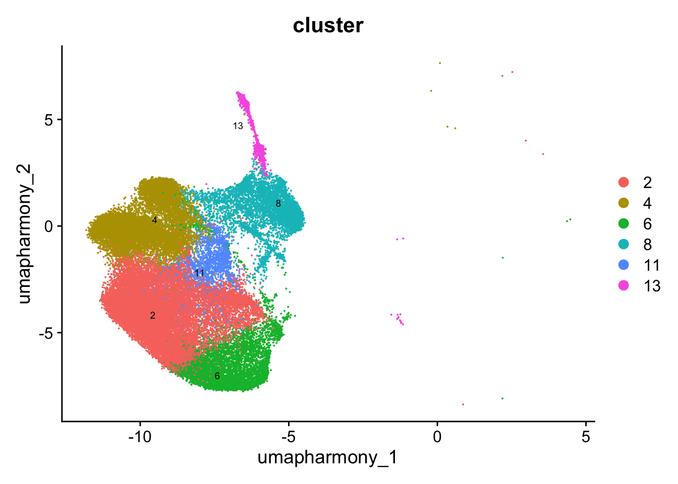
| Version | Author | Date |
|---|---|---|
| a94371e | Gunjan Dixit | 2024-06-07 |
paed_sub <- paed_sub %>%
  NormalizeData() %>%
  FindVariableFeatures() %>%
  ScaleData() %>%
  RunPCA()

paed_sub <- RunUMAP(paed_sub, dims = 1:30, reduction = "pca", reduction.name = "umap.new")
meta_data_columns <- colnames(paed_sub@meta.data)
columns_to_remove <- grep("^RNA_snn_res", meta_data_columns, value = TRUE)
paed_sub@meta.data <- paed_sub@meta.data[, !(colnames(paed_sub@meta.data) %in% columns_to_remove)]resolutions <- seq(0.1, 1, by = 0.1)
paed_sub <- FindNeighbors(paed_sub, dims = 1:30, reduction = "pca")
paed_sub <- FindClusters(paed_sub, resolution = resolutions )Modularity Optimizer version 1.3.0 by Ludo Waltman and Nees Jan van Eck
Number of nodes: 42503
Number of edges: 1301848
Running Louvain algorithm...
Maximum modularity in 10 random starts: 0.9540
Number of communities: 6
Elapsed time: 6 seconds
Modularity Optimizer version 1.3.0 by Ludo Waltman and Nees Jan van Eck
Number of nodes: 42503
Number of edges: 1301848
Running Louvain algorithm...
Maximum modularity in 10 random starts: 0.9338
Number of communities: 11
Elapsed time: 7 seconds
Modularity Optimizer version 1.3.0 by Ludo Waltman and Nees Jan van Eck
Number of nodes: 42503
Number of edges: 1301848
Running Louvain algorithm...
Maximum modularity in 10 random starts: 0.9218
Number of communities: 14
Elapsed time: 7 seconds
Modularity Optimizer version 1.3.0 by Ludo Waltman and Nees Jan van Eck
Number of nodes: 42503
Number of edges: 1301848
Running Louvain algorithm...
Maximum modularity in 10 random starts: 0.9108
Number of communities: 16
Elapsed time: 7 seconds
Modularity Optimizer version 1.3.0 by Ludo Waltman and Nees Jan van Eck
Number of nodes: 42503
Number of edges: 1301848
Running Louvain algorithm...
Maximum modularity in 10 random starts: 0.9010
Number of communities: 16
Elapsed time: 6 seconds
Modularity Optimizer version 1.3.0 by Ludo Waltman and Nees Jan van Eck
Number of nodes: 42503
Number of edges: 1301848
Running Louvain algorithm...
Maximum modularity in 10 random starts: 0.8913
Number of communities: 18
Elapsed time: 6 seconds
Modularity Optimizer version 1.3.0 by Ludo Waltman and Nees Jan van Eck
Number of nodes: 42503
Number of edges: 1301848
Running Louvain algorithm...
Maximum modularity in 10 random starts: 0.8824
Number of communities: 20
Elapsed time: 7 seconds
Modularity Optimizer version 1.3.0 by Ludo Waltman and Nees Jan van Eck
Number of nodes: 42503
Number of edges: 1301848
Running Louvain algorithm...
Maximum modularity in 10 random starts: 0.8752
Number of communities: 22
Elapsed time: 6 seconds
Modularity Optimizer version 1.3.0 by Ludo Waltman and Nees Jan van Eck
Number of nodes: 42503
Number of edges: 1301848
Running Louvain algorithm...
Maximum modularity in 10 random starts: 0.8673
Number of communities: 21
Elapsed time: 6 seconds
Modularity Optimizer version 1.3.0 by Ludo Waltman and Nees Jan van Eck
Number of nodes: 42503
Number of edges: 1301848
Running Louvain algorithm...
Maximum modularity in 10 random starts: 0.8596
Number of communities: 22
Elapsed time: 6 secondsclustree(paed_sub, prefix = "RNA_snn_res.")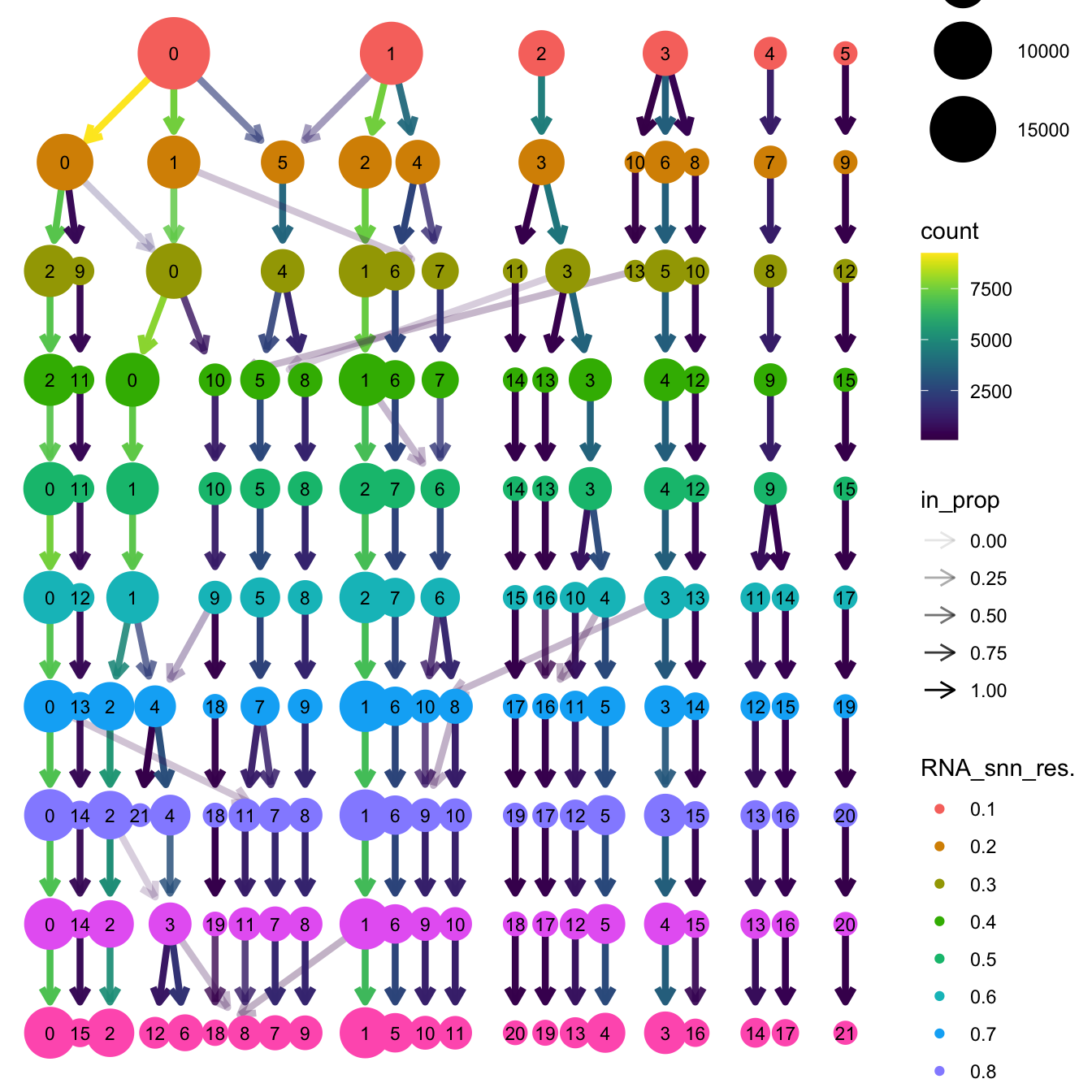
| Version | Author | Date |
|---|---|---|
| a94371e | Gunjan Dixit | 2024-06-07 |
# Visualize the clustering results
DimPlot(paed_sub, group.by = "RNA_snn_res.0.4", reduction = "umap.new", label = TRUE, label.size = 2.5, repel = TRUE, raster = FALSE )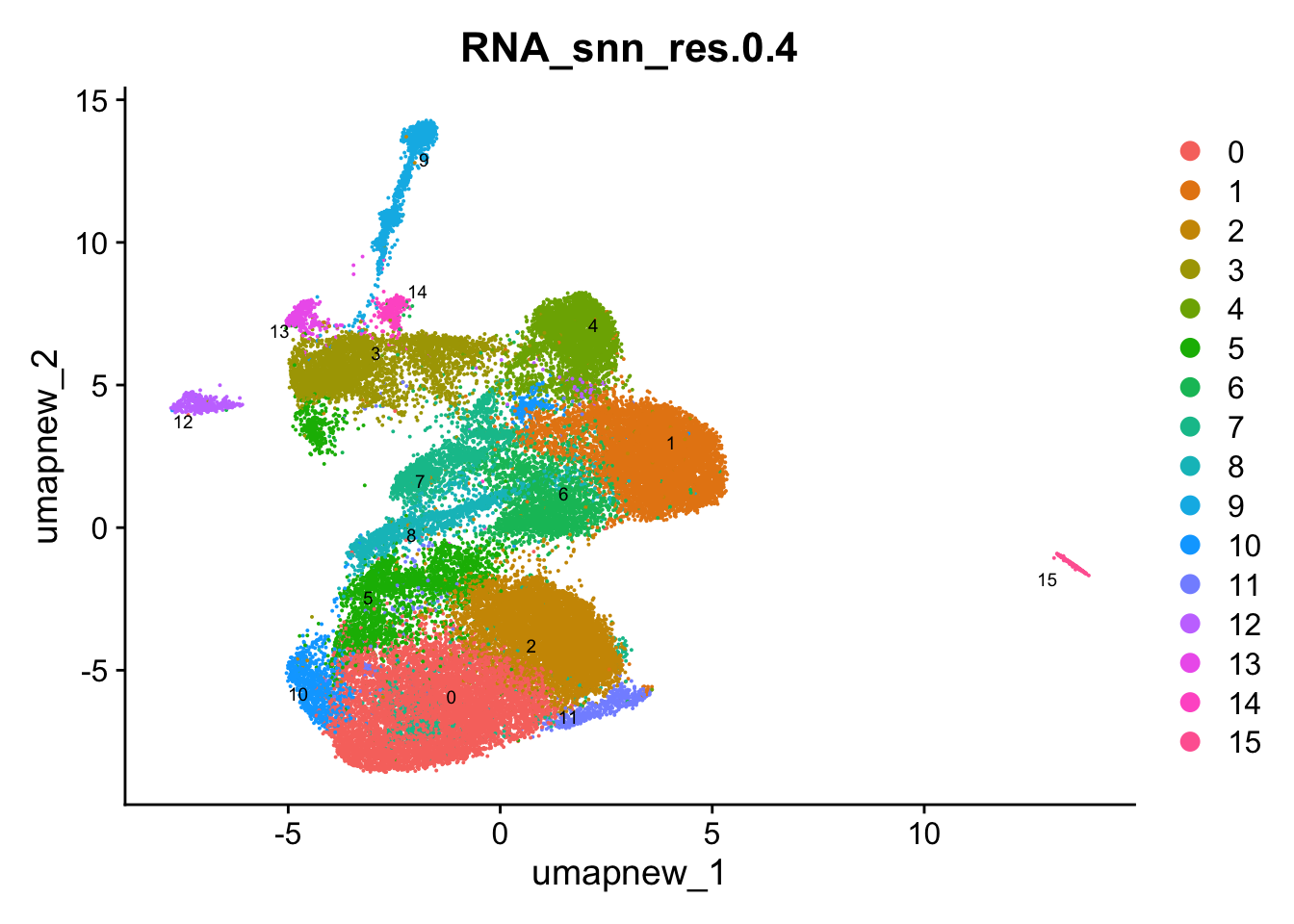
opt_res <- "RNA_snn_res.0.4"
n <- nlevels(paed_sub$RNA_snn_res.0.4)
paed_sub$RNA_snn_res.0.4 <- factor(paed_sub$RNA_snn_res.0.4, levels = seq(0,n-1))
paed_sub$seurat_clusters <- NULL
paed_sub$cluster <- paed_sub$RNA_snn_res.0.4
Idents(paed_sub) <- paed_sub$cluster
paed_sub.markers <- FindAllMarkers(paed_sub, only.pos = TRUE, min.pct = 0.25, logfc.threshold = 0.25)Calculating cluster 0Calculating cluster 1Calculating cluster 2Calculating cluster 3Calculating cluster 4Calculating cluster 5Calculating cluster 6Calculating cluster 7Calculating cluster 8Calculating cluster 9Calculating cluster 10Calculating cluster 11Calculating cluster 12Calculating cluster 13Calculating cluster 14Calculating cluster 15paed_sub.markers %>%
group_by(cluster) %>% unique() %>%
top_n(n = 5, wt = avg_log2FC) -> top5
paed_sub.markers %>%
group_by(cluster) %>%
slice_head(n=1) %>%
pull(gene) -> best.wilcox.gene.per.cluster
best.wilcox.gene.per.cluster [1] "TOX2" "KLF2" "GPR183" "CCL5" "CD8A" "MAF" "KLF2" "IFI44L"
[9] "FOXP3" "TRDC" "EGR2" "ACTB" "GZMK" "CCL5" "NKG7" "MS4A1" Violin plot shows the expression of top marker gene per cluster.
VlnPlot(paed_sub, features=best.wilcox.gene.per.cluster, ncol = 2, raster = FALSE, pt.size = FALSE)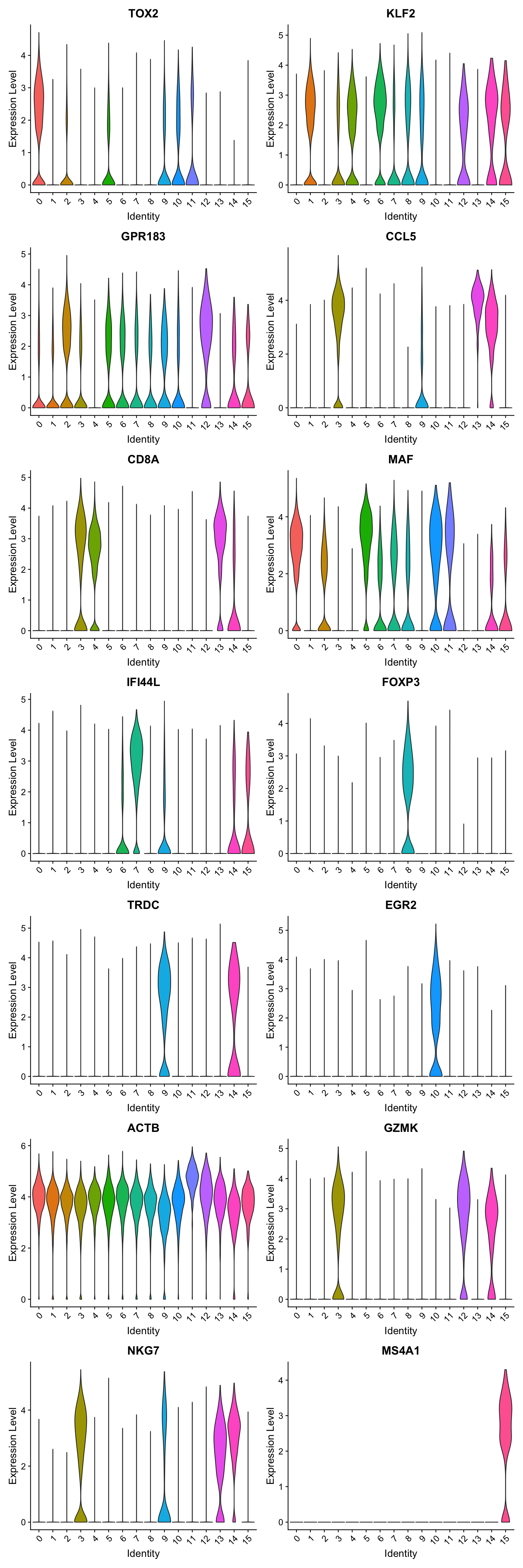
Feature plot shows the expression of top marker genes per cluster.
FeaturePlot(paed_sub,features=best.wilcox.gene.per.cluster, reduction = 'umap.new', raster = FALSE, ncol = 3, label = TRUE)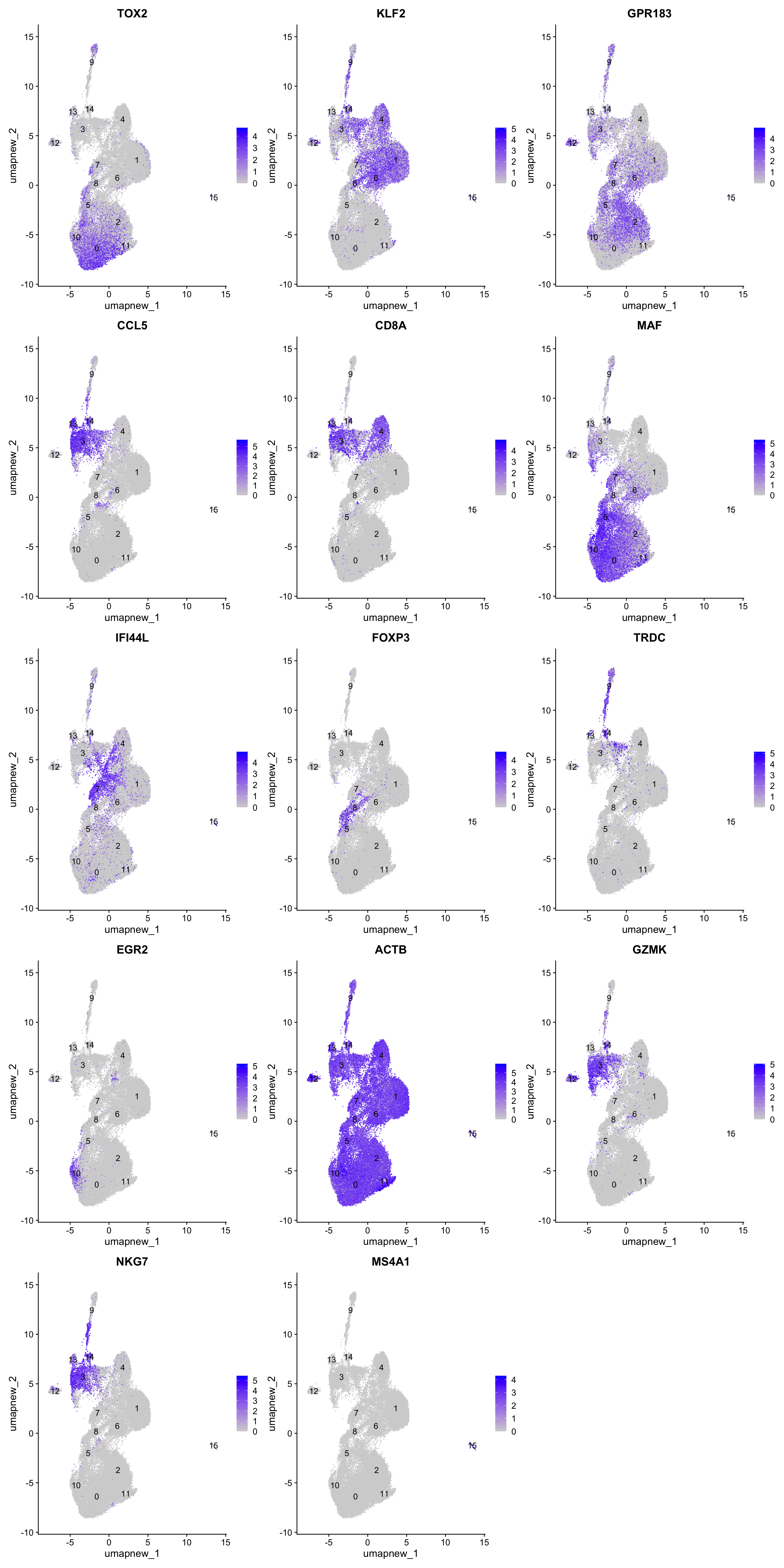
Top 10 marker genes from Seurat
## Seurat top markers
top10 <- paed_sub.markers %>%
    group_by(cluster) %>%
    top_n(n = 10, wt = avg_log2FC) %>%
    ungroup() %>%
    distinct(gene, .keep_all = TRUE) %>%
    arrange(cluster, desc(avg_log2FC))

cluster_colors <- paletteer::paletteer_d("pals::glasbey")[factor(top10$cluster)]

DotPlot(paed_sub,
        features = unique(top10$gene),
        group.by = opt_res,
        cols = c("azure1", "blueviolet"),
        dot.scale = 3, assay = "RNA") +
    RotatedAxis() +
    FontSize(y.text = 8, x.text = 12) +
    labs(y = element_blank(), x = element_blank()) +
    coord_flip() +
    theme(axis.text.y = element_text(color = cluster_colors)) +
    ggtitle("Top 10 marker genes per cluster (Seurat)")
Warning: Vectorized input to `element_text()` is not officially supported.
ℹ Results may be unexpected or may change in future versions of ggplot2.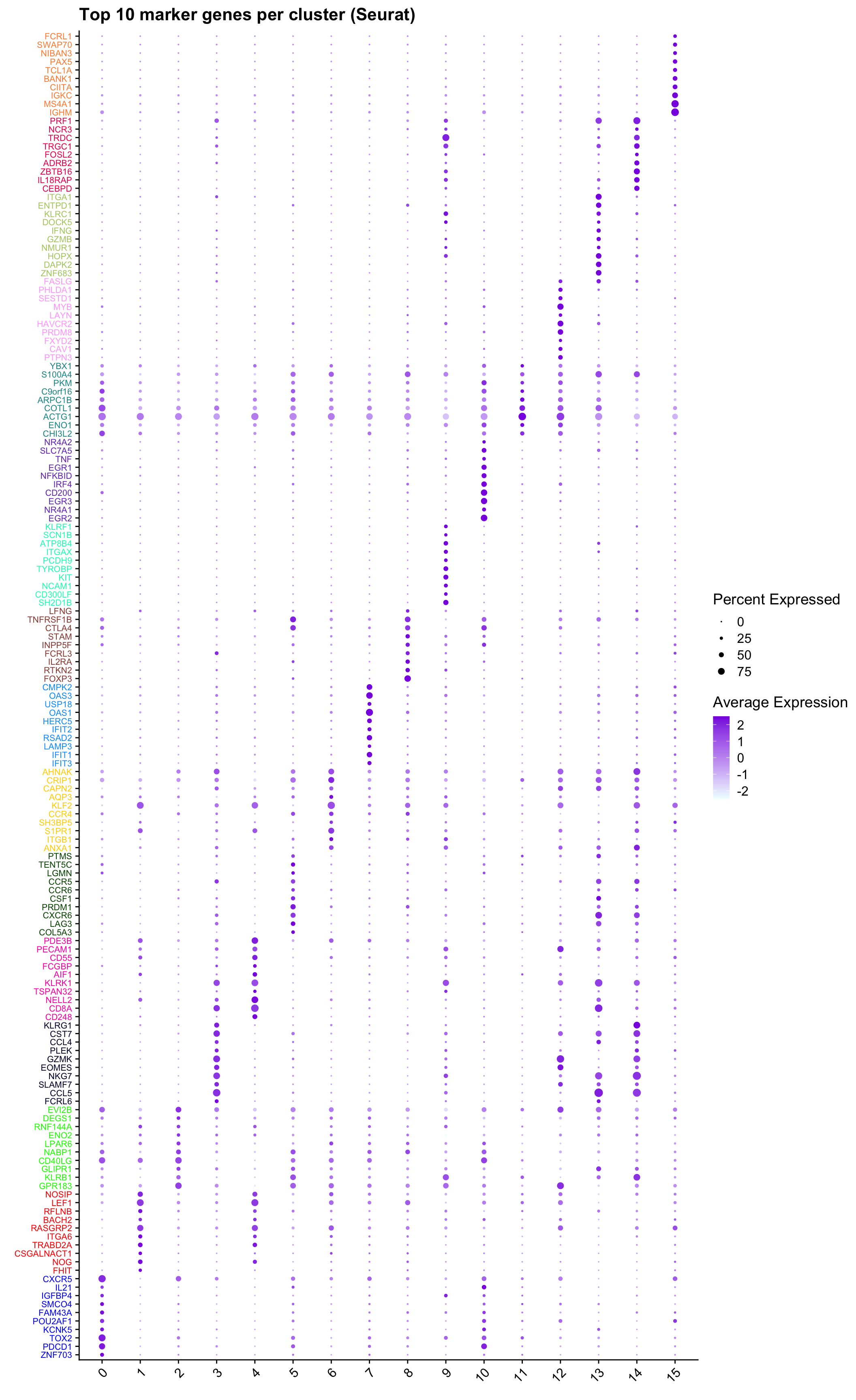
out_markers <- here("output",
            "CSV",
            paste(tissue,"_Marker_genes_Reclustered_Tcell_population.",opt_res, sep = ""))

dir.create(out_markers, recursive = TRUE, showWarnings = FALSE)

for (cl in unique(paed_sub.markers$cluster)) {
  cluster_data <- paed_sub.markers %>% dplyr::filter(cluster == cl)
  file_name <- here(out_markers, paste0("G000231_Neeland_",tissue, "_cluster_", cl, ".csv"))
  write.csv(cluster_data, file = file_name)
}
Corresponding Azimuth labels (T cell subsets)
## Level 1
DimPlot(paed_sub, reduction = "umap.new", group.by = "predicted.celltype.l1", raster = FALSE, repel = TRUE, label = TRUE, label.size = 4.5) 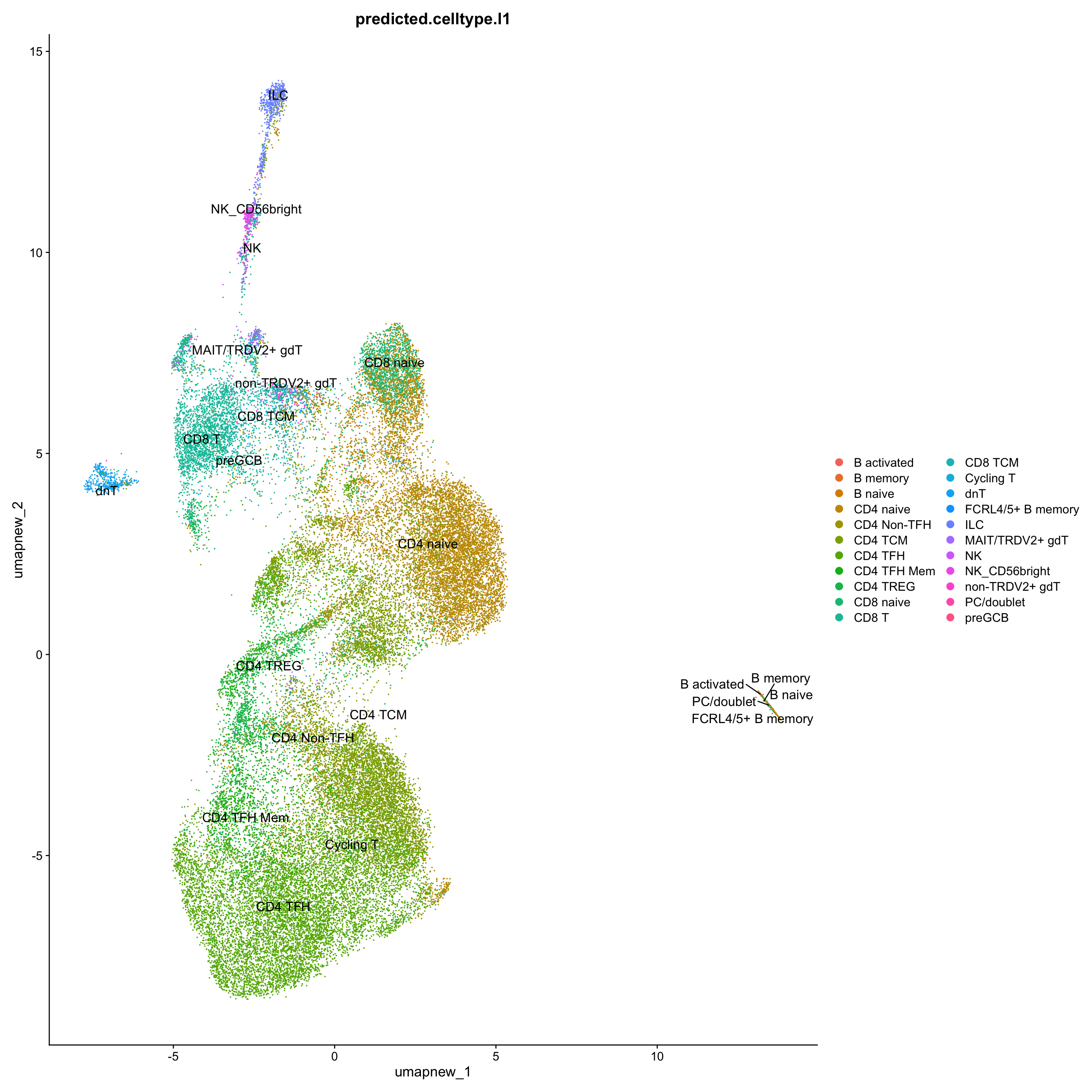
Excluding contaminating cells (B cell subtypes) for further clarity
sort(table(paed_sub$predicted.celltype.l1), decreasing = T)
          CD4 TFH           CD4 TCM         CD4 naive             CD8 T
            10935              9419              9316              2934
         CD4 TREG       CD4 TFH Mem       CD4 Non-TFH         CD8 naive
             2165              1878              1510              1408
          CD8 TCM               ILC               dnT     NK_CD56bright
              977               626               569               233
   non-TRDV2+ gdT   MAIT/TRDV2+ gdT           B naive                NK
              175               152               103                65
      B activated          B memory         Cycling T FCRL4/5+ B memory
               14                10                10                 2
       PC/doublet            preGCB
                1                 1
exclude <- c("B activated", "B memory", "B naive", "FCRL4/5+ B memory", "PC/doublet", "preGCB")
paed_sub_filtered <- paed_sub[, !paed_sub$predicted.celltype.l1 %in% exclude]
# Plots for Level 1
DimPlot(paed_sub_filtered, reduction = "umap.new", group.by = "predicted.celltype.l1", raster = FALSE, repel = TRUE, label = TRUE, label.size = 5) +
paletteer::scale_colour_paletteer_d("Polychrome::palette36")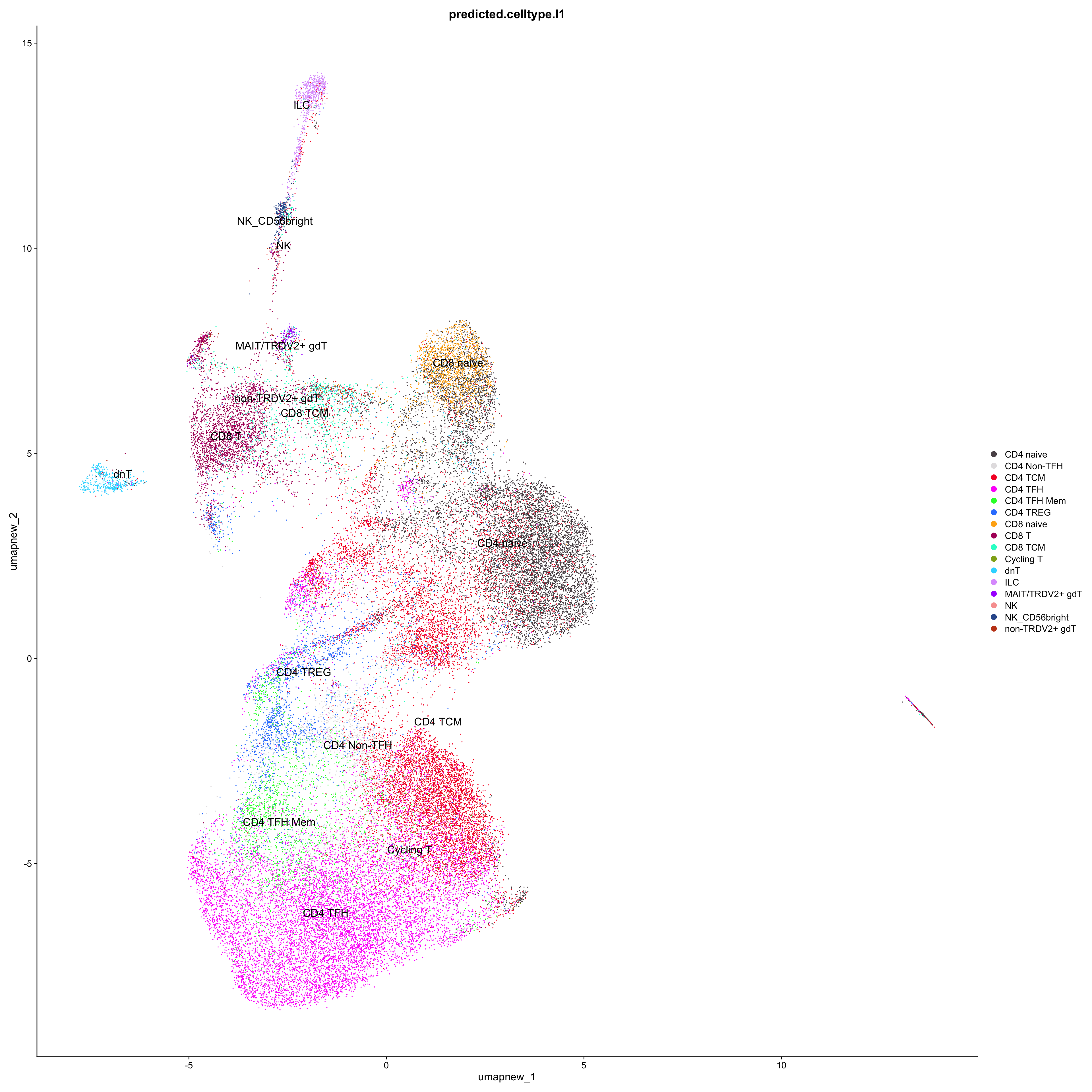
df_table_l1 <- as.data.frame(table(paed_sub_filtered$RNA_snn_res.0.4, paed_sub_filtered$predicted.celltype.l1))

ggplot(df_table_l1, aes(Var1, Freq, fill = Var2)) +
  geom_bar(stat = "identity") +
  labs(x = "RNA_snn_res.0.4", y = "Count", fill = "predicted.celltype.l1") +
  theme_minimal() +
  paletteer::scale_fill_paletteer_d("Polychrome::palette36") +
  ggtitle("Stacked Bar Plot of Tcell subsets (res=0.4) and predicted.celltype.l1")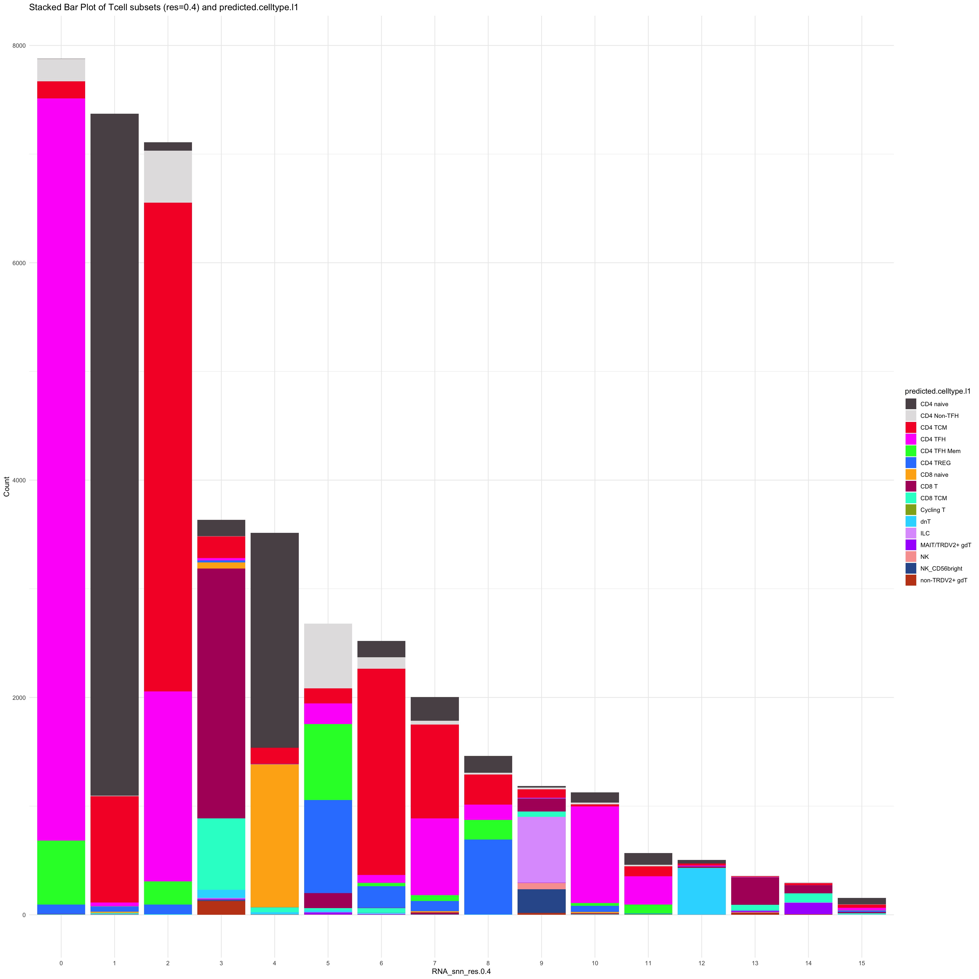
| Version | Author | Date |
|---|---|---|
| 649de68 | Gunjan Dixit | 2024-07-19 |
# Plots for Level 2
DimPlot(paed_sub_filtered, reduction = "umap.new", group.by = "predicted.celltype.l2", raster = FALSE, repel = TRUE, label = TRUE, label.size = 5)  +
    paletteer::scale_colour_paletteer_d("Polychrome::palette36")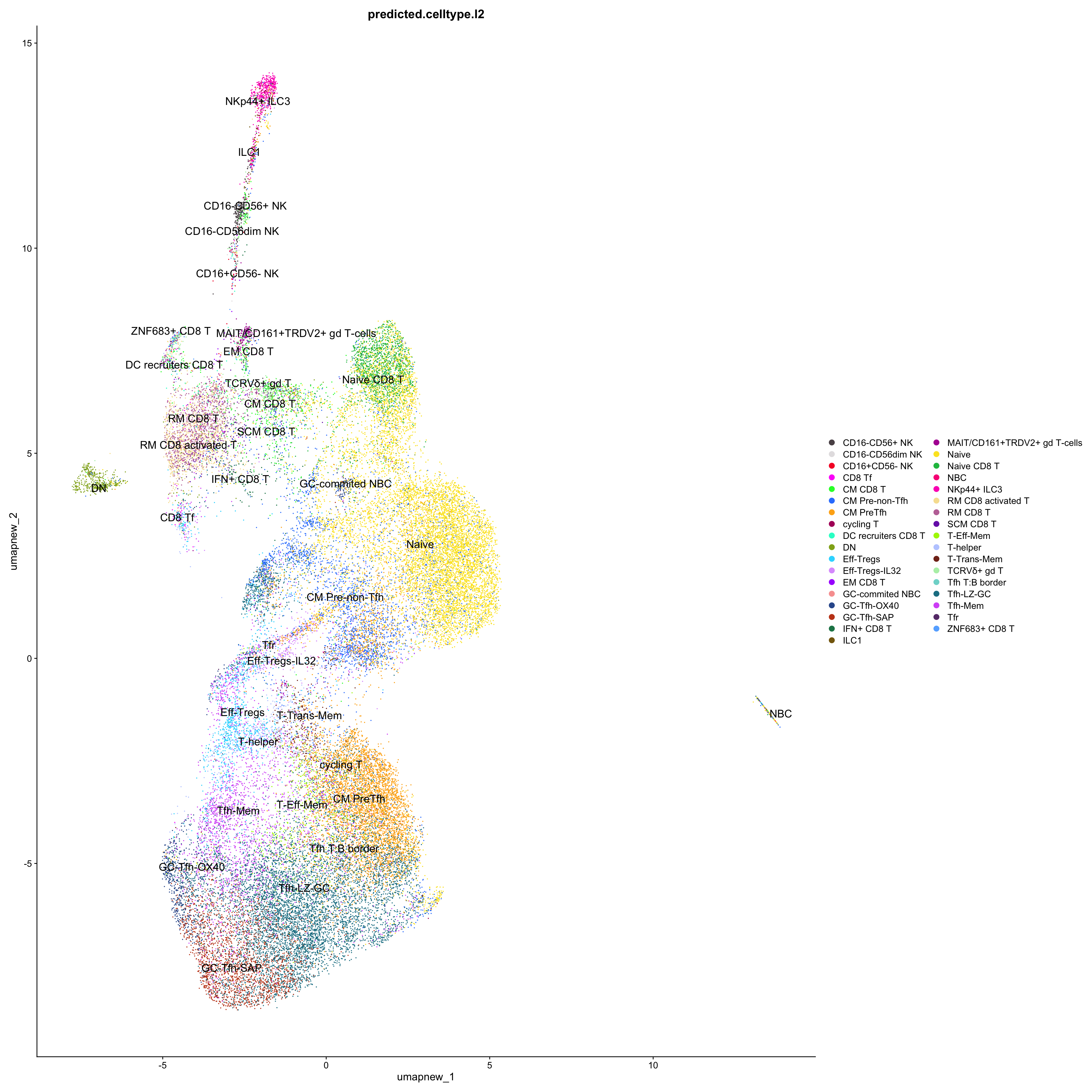
| Version | Author | Date |
|---|---|---|
| 649de68 | Gunjan Dixit | 2024-07-19 |
df_table_l2 <- as.data.frame(table(paed_sub_filtered$RNA_snn_res.0.4, paed_sub_filtered$predicted.celltype.l2))

ggplot(df_table_l2, aes(Var1, Freq, fill = Var2)) +
  geom_bar(stat = "identity") +
  labs(x = "RNA_snn_res.0.4", y = "Count", fill = "predicted.celltype.l2") +
  theme_minimal() +
  paletteer::scale_fill_paletteer_d("Polychrome::palette36") +
  ggtitle("Stacked Bar Plot of Tcell subsets (res=0.4) and predicted.celltype.l2")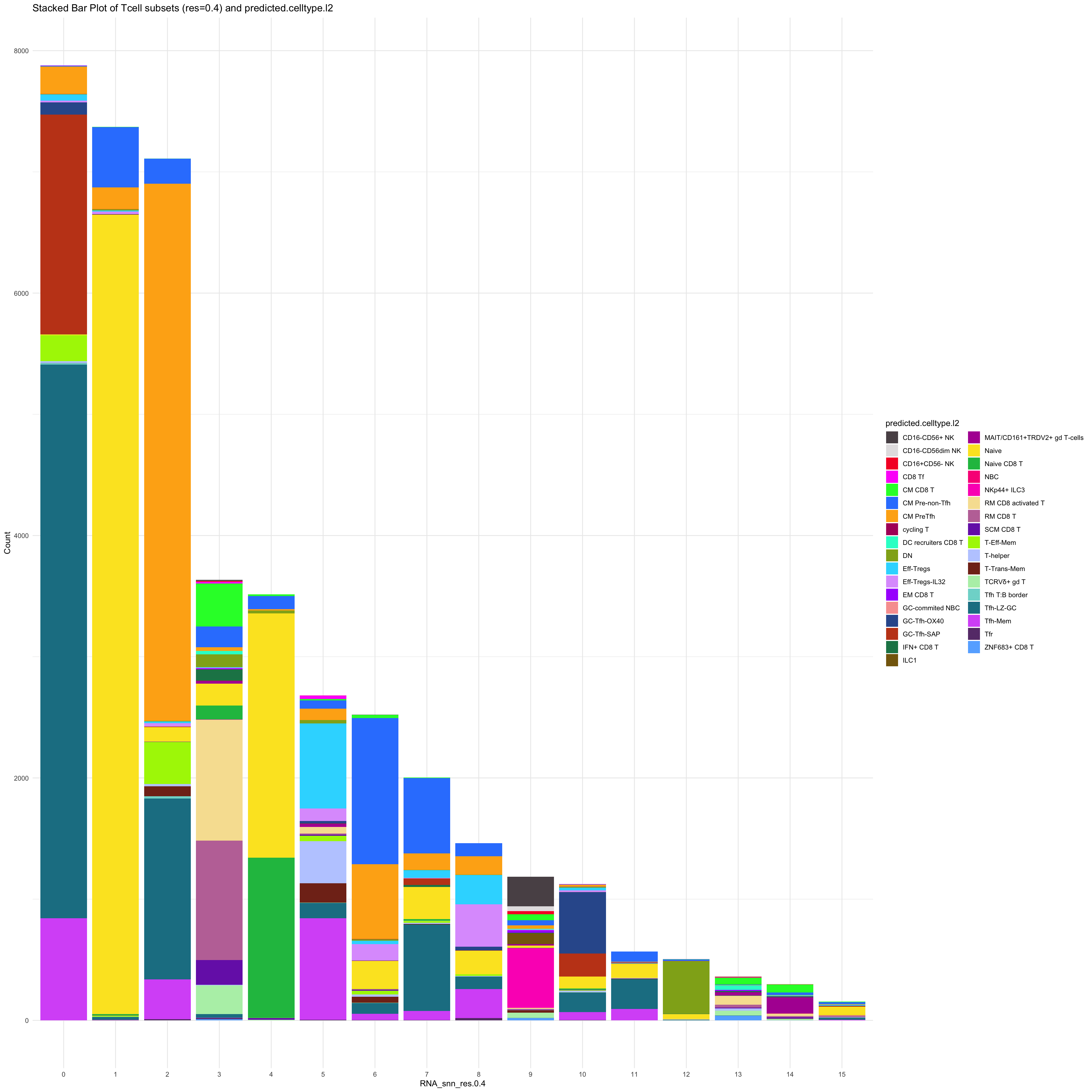
| Version | Author | Date |
|---|---|---|
| 649de68 | Gunjan Dixit | 2024-07-19 |
Reclustering Germinal Center B cells
Reclustering clusters 3,5,9
The marker genes for this reclustering can be found here-
Adenoids_GC_population_res.0.6
sub_clusters <- c(3,5,9)

idx <- which(merged_obj$cluster %in% sub_clusters)
paed_sub <- merged_obj[,idx]
paed_sub
An object of class Seurat
17456 features across 25451 samples within 1 assay
Active assay: RNA (17456 features, 2000 variable features)
3 layers present: data, counts, scale.data
4 dimensional reductions calculated: pca, umap.unintegrated, harmony, umap.harmony# Visualize the clustering results
DimPlot(paed_sub, reduction = "umap.harmony", group.by = "cluster", label = TRUE, label.size = 2.5, repel = TRUE, raster = FALSE )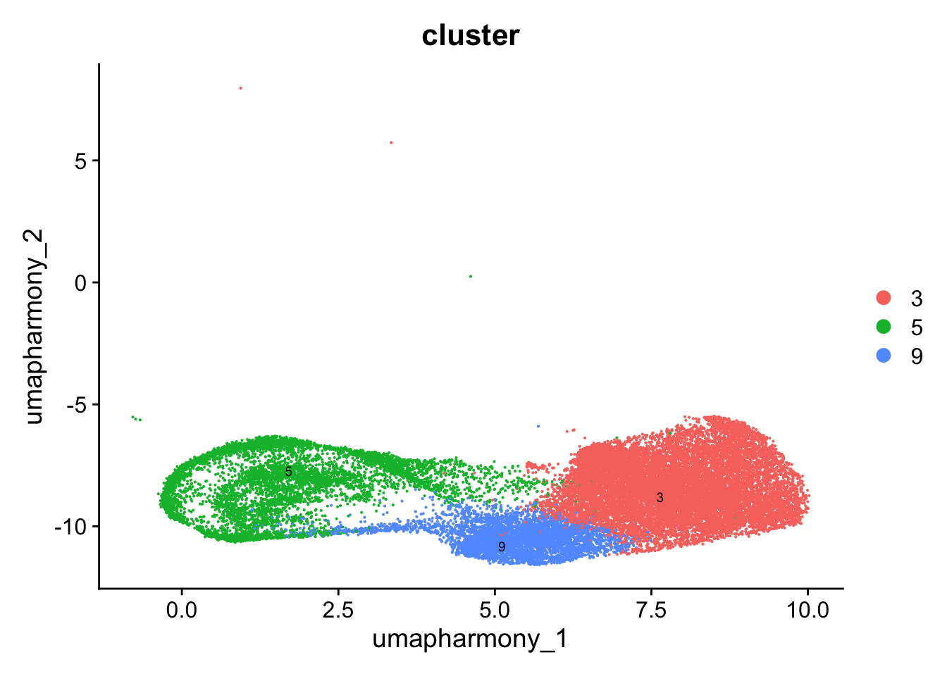
| Version | Author | Date |
|---|---|---|
| 649de68 | Gunjan Dixit | 2024-07-19 |
paed_sub <- paed_sub %>%
  NormalizeData() %>%
  FindVariableFeatures() %>%
  ScaleData() %>%
  RunPCA()

paed_sub <- RunUMAP(paed_sub, dims = 1:30, reduction = "pca", reduction.name = "umap.new")
meta_data_columns <- colnames(paed_sub@meta.data)
columns_to_remove <- grep("^RNA_snn_res", meta_data_columns, value = TRUE)
paed_sub@meta.data <- paed_sub@meta.data[, !(colnames(paed_sub@meta.data) %in% columns_to_remove)]resolutions <- seq(0.1, 1, by = 0.1)
paed_sub <- FindNeighbors(paed_sub, dims = 1:30, reduction = "pca")
paed_sub <- FindClusters(paed_sub, resolution = resolutions )Modularity Optimizer version 1.3.0 by Ludo Waltman and Nees Jan van Eck
Number of nodes: 25451
Number of edges: 785374
Running Louvain algorithm...
Maximum modularity in 10 random starts: 0.9400
Number of communities: 3
Elapsed time: 3 seconds
Modularity Optimizer version 1.3.0 by Ludo Waltman and Nees Jan van Eck
Number of nodes: 25451
Number of edges: 785374
Running Louvain algorithm...
Maximum modularity in 10 random starts: 0.9065
Number of communities: 5
Elapsed time: 4 seconds
Modularity Optimizer version 1.3.0 by Ludo Waltman and Nees Jan van Eck
Number of nodes: 25451
Number of edges: 785374
Running Louvain algorithm...
Maximum modularity in 10 random starts: 0.8875
Number of communities: 7
Elapsed time: 4 seconds
Modularity Optimizer version 1.3.0 by Ludo Waltman and Nees Jan van Eck
Number of nodes: 25451
Number of edges: 785374
Running Louvain algorithm...
Maximum modularity in 10 random starts: 0.8694
Number of communities: 8
Elapsed time: 4 seconds
Modularity Optimizer version 1.3.0 by Ludo Waltman and Nees Jan van Eck
Number of nodes: 25451
Number of edges: 785374
Running Louvain algorithm...
Maximum modularity in 10 random starts: 0.8567
Number of communities: 10
Elapsed time: 3 seconds
Modularity Optimizer version 1.3.0 by Ludo Waltman and Nees Jan van Eck
Number of nodes: 25451
Number of edges: 785374
Running Louvain algorithm...
Maximum modularity in 10 random starts: 0.8463
Number of communities: 13
Elapsed time: 4 seconds
Modularity Optimizer version 1.3.0 by Ludo Waltman and Nees Jan van Eck
Number of nodes: 25451
Number of edges: 785374
Running Louvain algorithm...
Maximum modularity in 10 random starts: 0.8357
Number of communities: 15
Elapsed time: 3 seconds
Modularity Optimizer version 1.3.0 by Ludo Waltman and Nees Jan van Eck
Number of nodes: 25451
Number of edges: 785374
Running Louvain algorithm...
Maximum modularity in 10 random starts: 0.8249
Number of communities: 15
Elapsed time: 3 seconds
Modularity Optimizer version 1.3.0 by Ludo Waltman and Nees Jan van Eck
Number of nodes: 25451
Number of edges: 785374
Running Louvain algorithm...
Maximum modularity in 10 random starts: 0.8173
Number of communities: 17
Elapsed time: 3 seconds
Modularity Optimizer version 1.3.0 by Ludo Waltman and Nees Jan van Eck
Number of nodes: 25451
Number of edges: 785374
Running Louvain algorithm...
Maximum modularity in 10 random starts: 0.8088
Number of communities: 16
Elapsed time: 3 secondsclustree(paed_sub, prefix = "RNA_snn_res.")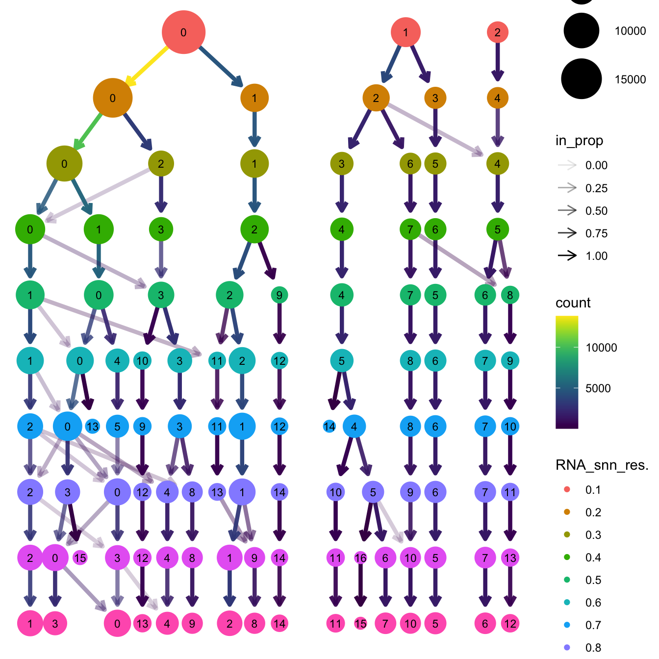
| Version | Author | Date |
|---|---|---|
| 649de68 | Gunjan Dixit | 2024-07-19 |
# Visualize the clustering results
DimPlot(paed_sub, group.by = "RNA_snn_res.0.6", reduction = "umap.new", label = TRUE, label.size = 2.5, repel = TRUE, raster = FALSE )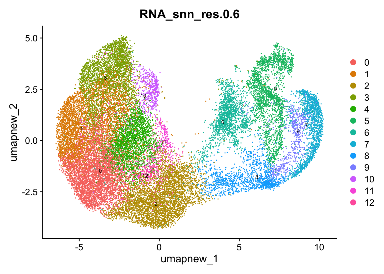
opt_res <- "RNA_snn_res.0.6"
n <- nlevels(paed_sub$RNA_snn_res.0.6)
paed_sub$RNA_snn_res.0.6 <- factor(paed_sub$RNA_snn_res.0.6, levels = seq(0,n-1))
paed_sub$seurat_clusters <- NULL
paed_sub$cluster <- paed_sub$RNA_snn_res.0.6
Idents(paed_sub) <- paed_sub$cluster
paed_sub.markers <- FindAllMarkers(paed_sub, only.pos = TRUE, min.pct = 0.25, logfc.threshold = 0.25)Calculating cluster 0Calculating cluster 1Calculating cluster 2Calculating cluster 3Calculating cluster 4Calculating cluster 5Calculating cluster 6Calculating cluster 7Calculating cluster 8Calculating cluster 9Calculating cluster 10Calculating cluster 11Calculating cluster 12paed_sub.markers %>%
group_by(cluster) %>% unique() %>%
top_n(n = 5, wt = avg_log2FC) -> top5
paed_sub.markers %>%
group_by(cluster) %>%
slice_head(n=1) %>%
pull(gene) -> best.wilcox.gene.per.cluster
best.wilcox.gene.per.cluster [1] "LMO2" "DDIT4" "AICDA" "BCL2A1" "CAMK1" "TYMS"
[7] "MCM4" "HIST1H2BB" "CDC20" "MKI67" "PRDM1" "RAB15"
[13] "PSAT1" Feature plot shows the expression of top marker genes per cluster.
FeaturePlot(paed_sub,features=best.wilcox.gene.per.cluster, reduction = 'umap.new', raster = FALSE, ncol = 2, label = TRUE)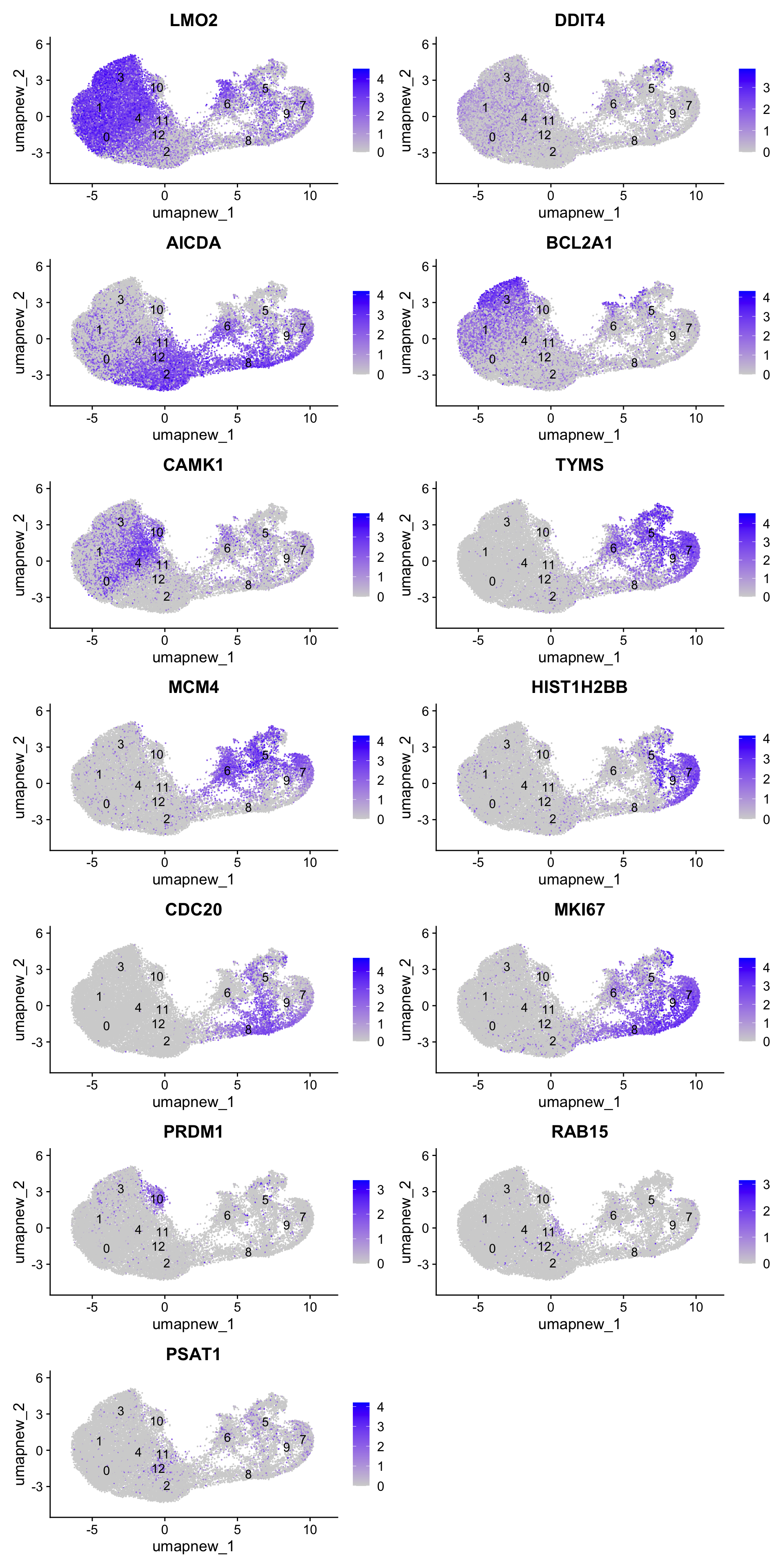
Top 10 marker genes from Seurat
## Seurat top markers
top10 <- paed_sub.markers %>%
    group_by(cluster) %>%
    top_n(n = 10, wt = avg_log2FC) %>%
    ungroup() %>%
    distinct(gene, .keep_all = TRUE) %>%
    arrange(cluster, desc(avg_log2FC))

cluster_colors <- paletteer::paletteer_d("pals::glasbey")[factor(top10$cluster)]

DotPlot(paed_sub,
        features = unique(top10$gene),
        group.by = opt_res,
        cols = c("azure1", "blueviolet"),
        dot.scale = 3, assay = "RNA") +
    RotatedAxis() +
    FontSize(y.text = 8, x.text = 12) +
    labs(y = element_blank(), x = element_blank()) +
    coord_flip() +
    theme(axis.text.y = element_text(color = cluster_colors)) +
    ggtitle("Top 10 marker genes per cluster (Seurat)")
Warning: Vectorized input to `element_text()` is not officially supported.
ℹ Results may be unexpected or may change in future versions of ggplot2.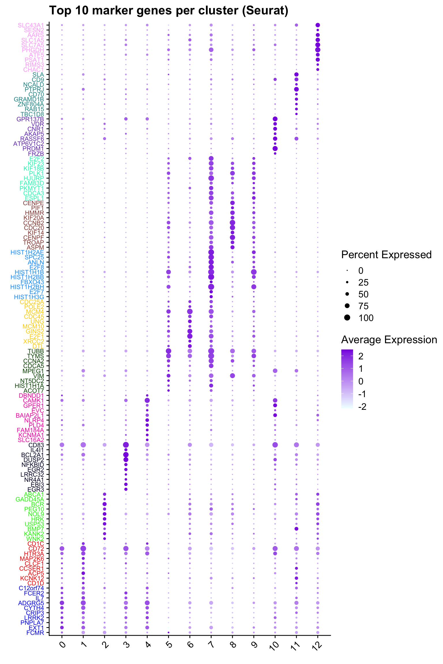
| Version | Author | Date |
|---|---|---|
| 649de68 | Gunjan Dixit | 2024-07-19 |
out_markers <- here("output",
            "CSV",
            paste(tissue,"_Marker_genes_Reclustered_GC_population.",opt_res, sep = ""))

dir.create(out_markers, recursive = TRUE, showWarnings = FALSE)

for (cl in unique(paed_sub.markers$cluster)) {
  cluster_data <- paed_sub.markers %>% dplyr::filter(cluster == cl)
  file_name <- here(out_markers, paste0("G000231_Neeland_",tissue, "_cluster_", cl, ".csv"))
  write.csv(cluster_data, file = file_name)
}
Corresponding Azimuth labels (GC cell subsets)
## Level 1
DimPlot(paed_sub, reduction = "umap.new", group.by = "predicted.celltype.l1", raster = FALSE, repel = TRUE, label = TRUE, label.size = 4.5) 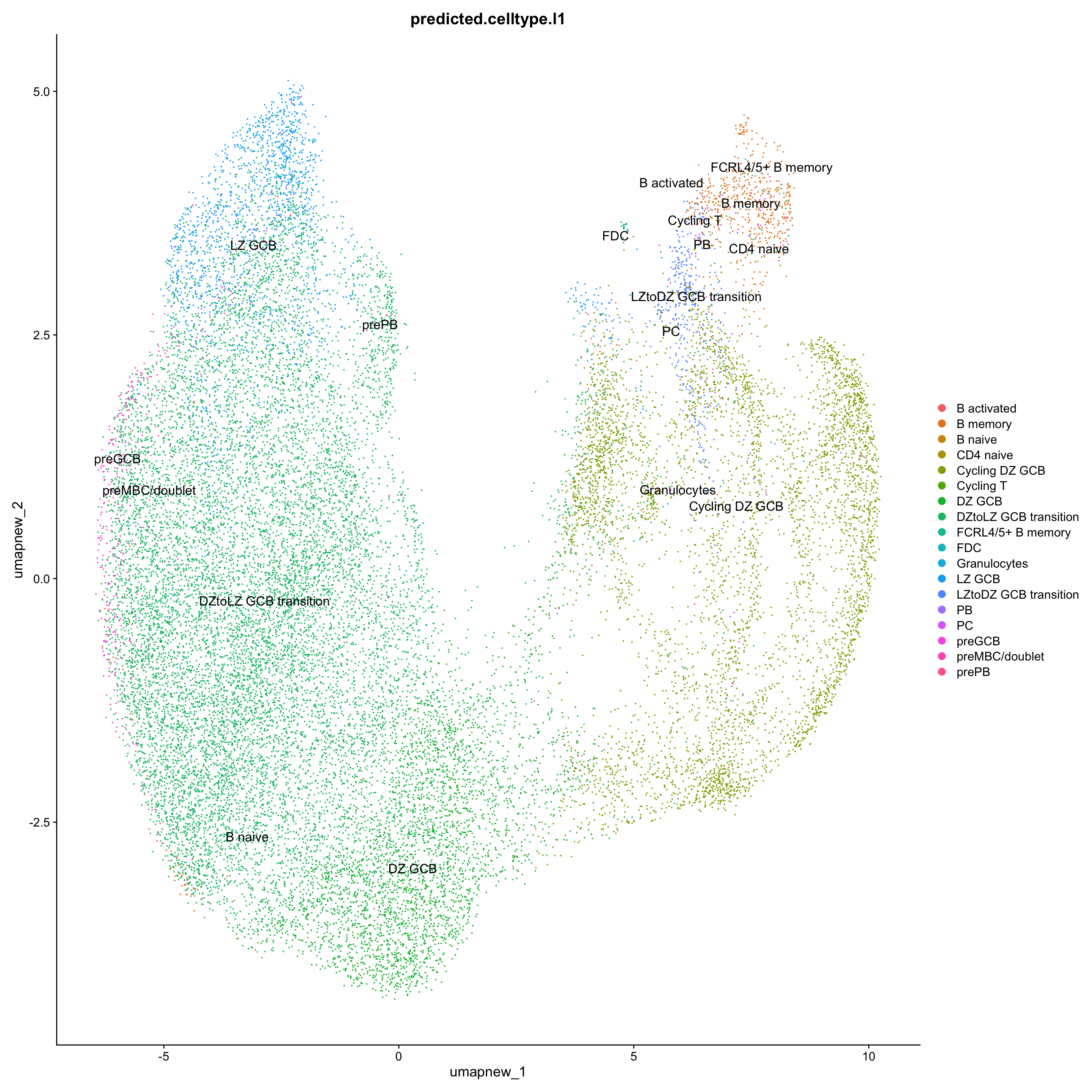
| Version | Author | Date |
|---|---|---|
| 649de68 | Gunjan Dixit | 2024-07-19 |
df_table <- as.data.frame(table(paed_sub$RNA_snn_res.0.6, paed_sub$predicted.celltype.l1))
ggplot(df_table, aes(Var1, Freq, fill = Var2)) +
  geom_bar(stat = "identity") +
  labs(x = "RNA_snn_res.0.6", y = "Count", fill = "predicted.celltype.l1") +
  theme_minimal() +
  ggtitle("Stacked Bar Plot of Tcell subsets (res=0.6) and predicted.celltype.l1")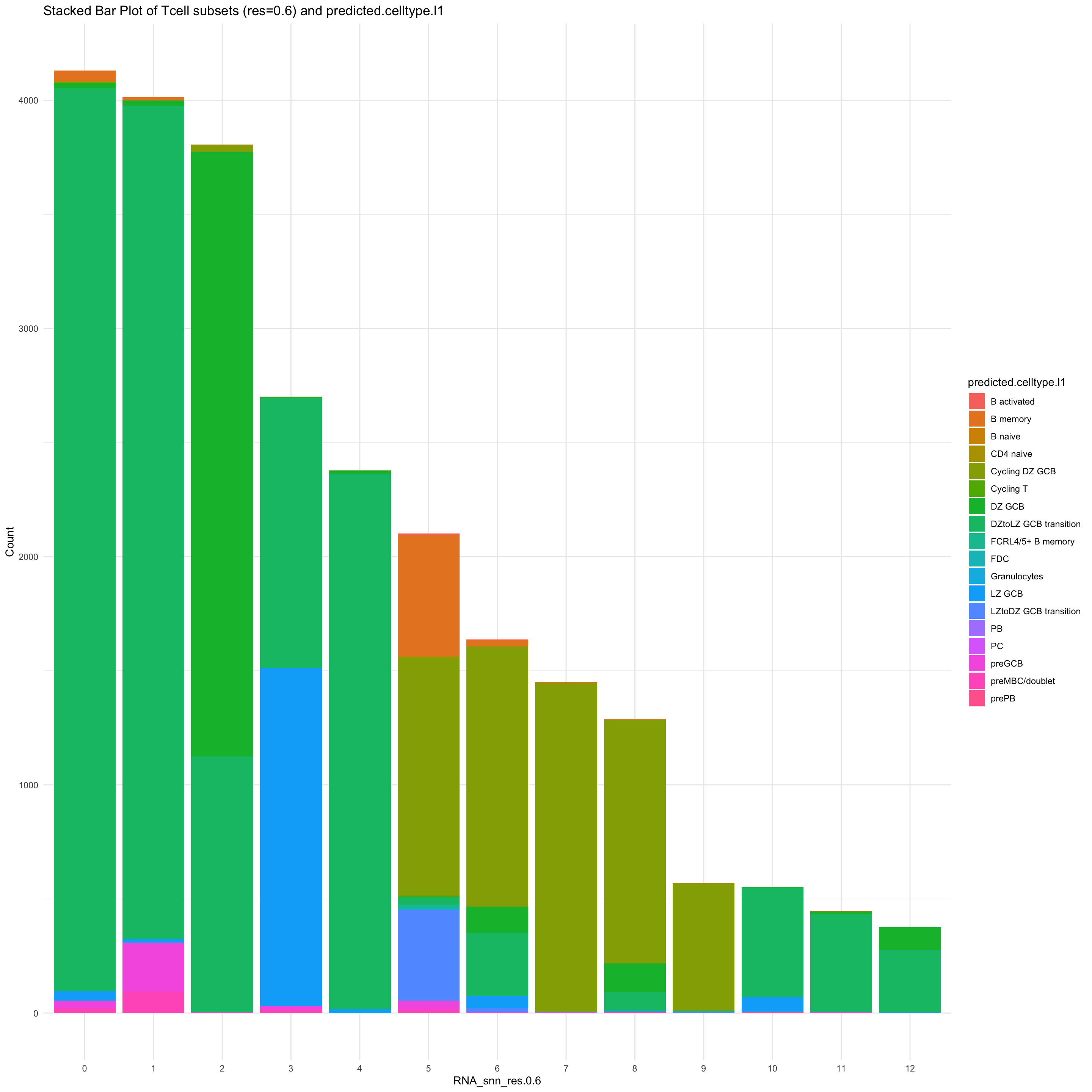
| Version | Author | Date |
|---|---|---|
| 649de68 | Gunjan Dixit | 2024-07-19 |
Confirm cluster 14 (activated DC3)
From Mel’s notes: Confirming CCR7 and LAMP3 expression in cluster 14 currently labelled as “activated DC3 (aDC3)?”
idx <- which(merged_obj$cluster %in% 14)
paed_sub <- merged_obj[,idx]
paed_sub
An object of class Seurat
17456 features across 859 samples within 1 assay
Active assay: RNA (17456 features, 2000 variable features)
3 layers present: data, counts, scale.data
4 dimensional reductions calculated: pca, umap.unintegrated, harmony, umap.harmonyFeaturePlot(paed_sub,features=c("CCR7","LAMP3"), reduction = 'umap.harmony', ncol = 1, label = FALSE)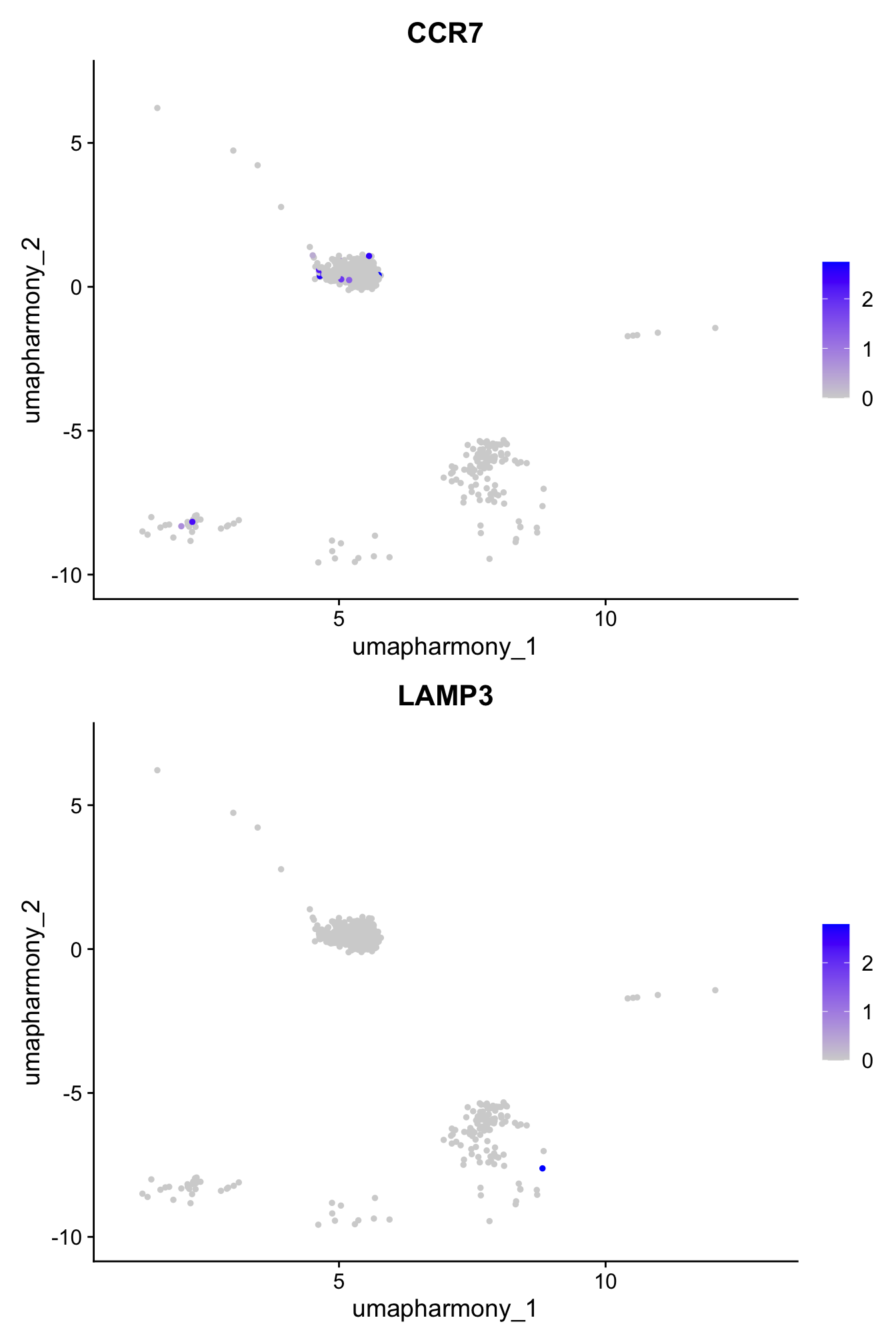
| Version | Author | Date |
|---|---|---|
| 649de68 | Gunjan Dixit | 2024-07-19 |
Session Info
sessioninfo::session_info()─ Session info ───────────────────────────────────────────────────────────────
setting value
version R version 4.3.2 (2023-10-31)
os macOS Sonoma 14.5
system aarch64, darwin20
ui X11
language (EN)
collate en_US.UTF-8
ctype en_US.UTF-8
tz Australia/Melbourne
date 2024-07-26
pandoc 3.1.1 @ /Users/dixitgunjan/Desktop/RStudio.app/Contents/Resources/app/quarto/bin/tools/ (via rmarkdown)
─ Packages ───────────────────────────────────────────────────────────────────
package * version date (UTC) lib source
abind 1.4-5 2016-07-21 [1] CRAN (R 4.3.0)
backports 1.4.1 2021-12-13 [1] CRAN (R 4.3.0)
beeswarm 0.4.0 2021-06-01 [1] CRAN (R 4.3.0)
BiocManager 1.30.22 2023-08-08 [1] CRAN (R 4.3.0)
BiocStyle * 2.30.0 2023-10-26 [1] Bioconductor
bslib 0.6.1 2023-11-28 [1] CRAN (R 4.3.1)
cachem 1.0.8 2023-05-01 [1] CRAN (R 4.3.0)
callr 3.7.5 2024-02-19 [1] CRAN (R 4.3.1)
cellranger 1.1.0 2016-07-27 [1] CRAN (R 4.3.0)
checkmate 2.3.1 2023-12-04 [1] CRAN (R 4.3.1)
cli 3.6.2 2023-12-11 [1] CRAN (R 4.3.1)
cluster 2.1.6 2023-12-01 [1] CRAN (R 4.3.1)
clustree * 0.5.1 2023-11-05 [1] CRAN (R 4.3.1)
codetools 0.2-19 2023-02-01 [1] CRAN (R 4.3.2)
colorspace 2.1-0 2023-01-23 [1] CRAN (R 4.3.0)
cowplot 1.1.3 2024-01-22 [1] CRAN (R 4.3.1)
data.table * 1.15.0 2024-01-30 [1] CRAN (R 4.3.1)
deldir 2.0-2 2023-11-23 [1] CRAN (R 4.3.1)
digest 0.6.34 2024-01-11 [1] CRAN (R 4.3.1)
dotCall64 1.1-1 2023-11-28 [1] CRAN (R 4.3.1)
dplyr * 1.1.4 2023-11-17 [1] CRAN (R 4.3.1)
ellipsis 0.3.2 2021-04-29 [1] CRAN (R 4.3.0)
evaluate 0.23 2023-11-01 [1] CRAN (R 4.3.1)
fansi 1.0.6 2023-12-08 [1] CRAN (R 4.3.1)
farver 2.1.1 2022-07-06 [1] CRAN (R 4.3.0)
fastDummies 1.7.3 2023-07-06 [1] CRAN (R 4.3.0)
fastmap 1.1.1 2023-02-24 [1] CRAN (R 4.3.0)
fitdistrplus 1.1-11 2023-04-25 [1] CRAN (R 4.3.0)
forcats * 1.0.0 2023-01-29 [1] CRAN (R 4.3.0)
fs 1.6.3 2023-07-20 [1] CRAN (R 4.3.0)
future 1.33.1 2023-12-22 [1] CRAN (R 4.3.1)
future.apply 1.11.1 2023-12-21 [1] CRAN (R 4.3.1)
generics 0.1.3 2022-07-05 [1] CRAN (R 4.3.0)
getPass 0.2-4 2023-12-10 [1] CRAN (R 4.3.1)
ggbeeswarm 0.7.2 2023-04-29 [1] CRAN (R 4.3.0)
ggforce 0.4.2 2024-02-19 [1] CRAN (R 4.3.1)
ggplot2 * 3.5.0 2024-02-23 [1] CRAN (R 4.3.1)
ggraph * 2.1.0 2022-10-09 [1] CRAN (R 4.3.0)
ggrastr 1.0.2 2023-06-01 [1] CRAN (R 4.3.0)
ggrepel 0.9.5 2024-01-10 [1] CRAN (R 4.3.1)
ggridges 0.5.6 2024-01-23 [1] CRAN (R 4.3.1)
git2r 0.33.0 2023-11-26 [1] CRAN (R 4.3.1)
globals 0.16.2 2022-11-21 [1] CRAN (R 4.3.0)
glue 1.7.0 2024-01-09 [1] CRAN (R 4.3.1)
goftest 1.2-3 2021-10-07 [1] CRAN (R 4.3.0)
graphlayouts 1.1.0 2024-01-19 [1] CRAN (R 4.3.1)
gridExtra 2.3 2017-09-09 [1] CRAN (R 4.3.0)
gtable 0.3.4 2023-08-21 [1] CRAN (R 4.3.0)
here * 1.0.1 2020-12-13 [1] CRAN (R 4.3.0)
highr 0.10 2022-12-22 [1] CRAN (R 4.3.0)
hms 1.1.3 2023-03-21 [1] CRAN (R 4.3.0)
htmltools 0.5.7 2023-11-03 [1] CRAN (R 4.3.1)
htmlwidgets 1.6.4 2023-12-06 [1] CRAN (R 4.3.1)
httpuv 1.6.14 2024-01-26 [1] CRAN (R 4.3.1)
httr 1.4.7 2023-08-15 [1] CRAN (R 4.3.0)
ica 1.0-3 2022-07-08 [1] CRAN (R 4.3.0)
igraph 2.0.2 2024-02-17 [1] CRAN (R 4.3.1)
irlba 2.3.5.1 2022-10-03 [1] CRAN (R 4.3.2)
jquerylib 0.1.4 2021-04-26 [1] CRAN (R 4.3.0)
jsonlite 1.8.8 2023-12-04 [1] CRAN (R 4.3.1)
kableExtra * 1.4.0 2024-01-24 [1] CRAN (R 4.3.1)
KernSmooth 2.23-22 2023-07-10 [1] CRAN (R 4.3.2)
knitr 1.45 2023-10-30 [1] CRAN (R 4.3.1)
labeling 0.4.3 2023-08-29 [1] CRAN (R 4.3.0)
later 1.3.2 2023-12-06 [1] CRAN (R 4.3.1)
lattice 0.22-5 2023-10-24 [1] CRAN (R 4.3.1)
lazyeval 0.2.2 2019-03-15 [1] CRAN (R 4.3.0)
leiden 0.4.3.1 2023-11-17 [1] CRAN (R 4.3.1)
lifecycle 1.0.4 2023-11-07 [1] CRAN (R 4.3.1)
limma 3.58.1 2023-11-02 [1] Bioconductor
listenv 0.9.1 2024-01-29 [1] CRAN (R 4.3.1)
lmtest 0.9-40 2022-03-21 [1] CRAN (R 4.3.0)
lubridate * 1.9.3 2023-09-27 [1] CRAN (R 4.3.1)
magrittr 2.0.3 2022-03-30 [1] CRAN (R 4.3.0)
MASS 7.3-60.0.1 2024-01-13 [1] CRAN (R 4.3.1)
Matrix 1.6-5 2024-01-11 [1] CRAN (R 4.3.1)
matrixStats 1.2.0 2023-12-11 [1] CRAN (R 4.3.1)
mime 0.12 2021-09-28 [1] CRAN (R 4.3.0)
miniUI 0.1.1.1 2018-05-18 [1] CRAN (R 4.3.0)
munsell 0.5.0 2018-06-12 [1] CRAN (R 4.3.0)
nlme 3.1-164 2023-11-27 [1] CRAN (R 4.3.1)
paletteer 1.6.0 2024-01-21 [1] CRAN (R 4.3.1)
parallelly 1.37.0 2024-02-14 [1] CRAN (R 4.3.1)
patchwork * 1.2.0 2024-01-08 [1] CRAN (R 4.3.1)
pbapply 1.7-2 2023-06-27 [1] CRAN (R 4.3.0)
pillar 1.9.0 2023-03-22 [1] CRAN (R 4.3.0)
pkgconfig 2.0.3 2019-09-22 [1] CRAN (R 4.3.0)
plotly 4.10.4 2024-01-13 [1] CRAN (R 4.3.1)
plyr 1.8.9 2023-10-02 [1] CRAN (R 4.3.1)
png 0.1-8 2022-11-29 [1] CRAN (R 4.3.0)
polyclip 1.10-6 2023-09-27 [1] CRAN (R 4.3.1)
presto 1.0.0 2024-02-27 [1] Github (immunogenomics/presto@31dc97f)
prismatic 1.1.1 2022-08-15 [1] CRAN (R 4.3.0)
processx 3.8.3 2023-12-10 [1] CRAN (R 4.3.1)
progressr 0.14.0 2023-08-10 [1] CRAN (R 4.3.0)
promises 1.2.1 2023-08-10 [1] CRAN (R 4.3.0)
ps 1.7.6 2024-01-18 [1] CRAN (R 4.3.1)
purrr * 1.0.2 2023-08-10 [1] CRAN (R 4.3.0)
R6 2.5.1 2021-08-19 [1] CRAN (R 4.3.0)
RANN 2.6.1 2019-01-08 [1] CRAN (R 4.3.0)
RColorBrewer * 1.1-3 2022-04-03 [1] CRAN (R 4.3.0)
Rcpp 1.0.12 2024-01-09 [1] CRAN (R 4.3.1)
RcppAnnoy 0.0.22 2024-01-23 [1] CRAN (R 4.3.1)
RcppHNSW 0.6.0 2024-02-04 [1] CRAN (R 4.3.1)
readr * 2.1.5 2024-01-10 [1] CRAN (R 4.3.1)
readxl * 1.4.3 2023-07-06 [1] CRAN (R 4.3.0)
rematch2 2.1.2 2020-05-01 [1] CRAN (R 4.3.0)
reshape2 1.4.4 2020-04-09 [1] CRAN (R 4.3.0)
reticulate 1.35.0 2024-01-31 [1] CRAN (R 4.3.1)
rlang 1.1.3 2024-01-10 [1] CRAN (R 4.3.1)
rmarkdown 2.25 2023-09-18 [1] CRAN (R 4.3.1)
ROCR 1.0-11 2020-05-02 [1] CRAN (R 4.3.0)
rprojroot 2.0.4 2023-11-05 [1] CRAN (R 4.3.1)
RSpectra 0.16-1 2022-04-24 [1] CRAN (R 4.3.0)
rstudioapi 0.15.0 2023-07-07 [1] CRAN (R 4.3.0)
Rtsne 0.17 2023-12-07 [1] CRAN (R 4.3.1)
sass 0.4.8 2023-12-06 [1] CRAN (R 4.3.1)
scales 1.3.0 2023-11-28 [1] CRAN (R 4.3.1)
scattermore 1.2 2023-06-12 [1] CRAN (R 4.3.0)
sctransform 0.4.1 2023-10-19 [1] CRAN (R 4.3.1)
sessioninfo 1.2.2 2021-12-06 [1] CRAN (R 4.3.0)
Seurat * 5.0.1.9009 2024-02-28 [1] Github (satijalab/seurat@6a3ef5e)
SeuratObject * 5.0.1 2023-11-17 [1] CRAN (R 4.3.1)
shiny 1.8.0 2023-11-17 [1] CRAN (R 4.3.1)
sp * 2.1-3 2024-01-30 [1] CRAN (R 4.3.1)
spam 2.10-0 2023-10-23 [1] CRAN (R 4.3.1)
spatstat.data 3.0-4 2024-01-15 [1] CRAN (R 4.3.1)
spatstat.explore 3.2-6 2024-02-01 [1] CRAN (R 4.3.1)
spatstat.geom 3.2-8 2024-01-26 [1] CRAN (R 4.3.1)
spatstat.random 3.2-2 2023-11-29 [1] CRAN (R 4.3.1)
spatstat.sparse 3.0-3 2023-10-24 [1] CRAN (R 4.3.1)
spatstat.utils 3.0-4 2023-10-24 [1] CRAN (R 4.3.1)
statmod 1.5.0 2023-01-06 [1] CRAN (R 4.3.0)
stringi 1.8.3 2023-12-11 [1] CRAN (R 4.3.1)
stringr * 1.5.1 2023-11-14 [1] CRAN (R 4.3.1)
survival 3.5-8 2024-02-14 [1] CRAN (R 4.3.1)
svglite 2.1.3 2023-12-08 [1] CRAN (R 4.3.1)
systemfonts 1.0.5 2023-10-09 [1] CRAN (R 4.3.1)
tensor 1.5 2012-05-05 [1] CRAN (R 4.3.0)
tibble * 3.2.1 2023-03-20 [1] CRAN (R 4.3.0)
tidygraph 1.3.1 2024-01-30 [1] CRAN (R 4.3.1)
tidyr * 1.3.1 2024-01-24 [1] CRAN (R 4.3.1)
tidyselect 1.2.0 2022-10-10 [1] CRAN (R 4.3.0)
tidyverse * 2.0.0 2023-02-22 [1] CRAN (R 4.3.0)
timechange 0.3.0 2024-01-18 [1] CRAN (R 4.3.1)
tweenr 2.0.3 2024-02-26 [1] CRAN (R 4.3.1)
tzdb 0.4.0 2023-05-12 [1] CRAN (R 4.3.0)
utf8 1.2.4 2023-10-22 [1] CRAN (R 4.3.1)
uwot 0.1.16 2023-06-29 [1] CRAN (R 4.3.0)
vctrs 0.6.5 2023-12-01 [1] CRAN (R 4.3.1)
vipor 0.4.7 2023-12-18 [1] CRAN (R 4.3.1)
viridis 0.6.5 2024-01-29 [1] CRAN (R 4.3.1)
viridisLite 0.4.2 2023-05-02 [1] CRAN (R 4.3.0)
whisker 0.4.1 2022-12-05 [1] CRAN (R 4.3.0)
withr 3.0.0 2024-01-16 [1] CRAN (R 4.3.1)
workflowr * 1.7.1 2023-08-23 [1] CRAN (R 4.3.0)
xfun 0.42 2024-02-08 [1] CRAN (R 4.3.1)
xml2 1.3.6 2023-12-04 [1] CRAN (R 4.3.1)
xtable 1.8-4 2019-04-21 [1] CRAN (R 4.3.0)
yaml 2.3.8 2023-12-11 [1] CRAN (R 4.3.1)
zoo 1.8-12 2023-04-13 [1] CRAN (R 4.3.0)
[1] /Library/Frameworks/R.framework/Versions/4.3-arm64/Resources/library
──────────────────────────────────────────────────────────────────────────────
sessionInfo()R version 4.3.2 (2023-10-31)
Platform: aarch64-apple-darwin20 (64-bit)
Running under: macOS Sonoma 14.5
Matrix products: default
BLAS: /Library/Frameworks/R.framework/Versions/4.3-arm64/Resources/lib/libRblas.0.dylib
LAPACK: /Library/Frameworks/R.framework/Versions/4.3-arm64/Resources/lib/libRlapack.dylib; LAPACK version 3.11.0
locale:
[1] en_US.UTF-8/en_US.UTF-8/en_US.UTF-8/C/en_US.UTF-8/en_US.UTF-8
time zone: Australia/Melbourne
tzcode source: internal
attached base packages:
[1] stats graphics grDevices utils datasets methods base
other attached packages:
[1] readxl_1.4.3 patchwork_1.2.0 data.table_1.15.0 RColorBrewer_1.1-3
[5] kableExtra_1.4.0 clustree_0.5.1 ggraph_2.1.0 Seurat_5.0.1.9009
[9] SeuratObject_5.0.1 sp_2.1-3 here_1.0.1 lubridate_1.9.3
[13] forcats_1.0.0 stringr_1.5.1 dplyr_1.1.4 purrr_1.0.2
[17] readr_2.1.5 tidyr_1.3.1 tibble_3.2.1 ggplot2_3.5.0
[21] tidyverse_2.0.0 BiocStyle_2.30.0 workflowr_1.7.1
loaded via a namespace (and not attached):
[1] RcppAnnoy_0.0.22 splines_4.3.2 later_1.3.2
[4] prismatic_1.1.1 cellranger_1.1.0 polyclip_1.10-6
[7] fastDummies_1.7.3 lifecycle_1.0.4 rprojroot_2.0.4
[10] globals_0.16.2 processx_3.8.3 lattice_0.22-5
[13] MASS_7.3-60.0.1 backports_1.4.1 magrittr_2.0.3
[16] limma_3.58.1 plotly_4.10.4 sass_0.4.8
[19] rmarkdown_2.25 jquerylib_0.1.4 yaml_2.3.8
[22] httpuv_1.6.14 sctransform_0.4.1 spam_2.10-0
[25] sessioninfo_1.2.2 spatstat.sparse_3.0-3 reticulate_1.35.0
[28] cowplot_1.1.3 pbapply_1.7-2 abind_1.4-5
[31] Rtsne_0.17 presto_1.0.0 tweenr_2.0.3
[34] git2r_0.33.0 ggrepel_0.9.5 irlba_2.3.5.1
[37] listenv_0.9.1 spatstat.utils_3.0-4 goftest_1.2-3
[40] RSpectra_0.16-1 spatstat.random_3.2-2 fitdistrplus_1.1-11
[43] parallelly_1.37.0 svglite_2.1.3 leiden_0.4.3.1
[46] codetools_0.2-19 xml2_1.3.6 ggforce_0.4.2
[49] tidyselect_1.2.0 farver_2.1.1 viridis_0.6.5
[52] matrixStats_1.2.0 spatstat.explore_3.2-6 jsonlite_1.8.8
[55] ellipsis_0.3.2 tidygraph_1.3.1 progressr_0.14.0
[58] ggridges_0.5.6 survival_3.5-8 systemfonts_1.0.5
[61] tools_4.3.2 ica_1.0-3 Rcpp_1.0.12
[64] glue_1.7.0 gridExtra_2.3 xfun_0.42
[67] withr_3.0.0 BiocManager_1.30.22 fastmap_1.1.1
[70] fansi_1.0.6 callr_3.7.5 digest_0.6.34
[73] timechange_0.3.0 R6_2.5.1 mime_0.12
[76] colorspace_2.1-0 scattermore_1.2 tensor_1.5
[79] spatstat.data_3.0-4 utf8_1.2.4 generics_0.1.3
[82] graphlayouts_1.1.0 httr_1.4.7 htmlwidgets_1.6.4
[85] whisker_0.4.1 uwot_0.1.16 pkgconfig_2.0.3
[88] gtable_0.3.4 lmtest_0.9-40 htmltools_0.5.7
[91] dotCall64_1.1-1 scales_1.3.0 png_0.1-8
[94] knitr_1.45 rstudioapi_0.15.0 tzdb_0.4.0
[97] reshape2_1.4.4 checkmate_2.3.1 nlme_3.1-164
[100] cachem_1.0.8 zoo_1.8-12 KernSmooth_2.23-22
[103] vipor_0.4.7 parallel_4.3.2 miniUI_0.1.1.1
[106] ggrastr_1.0.2 pillar_1.9.0 grid_4.3.2
[109] vctrs_0.6.5 RANN_2.6.1 promises_1.2.1
[112] xtable_1.8-4 cluster_2.1.6 paletteer_1.6.0
[115] beeswarm_0.4.0 evaluate_0.23 cli_3.6.2
[118] compiler_4.3.2 rlang_1.1.3 future.apply_1.11.1
[121] labeling_0.4.3 rematch2_2.1.2 ps_1.7.6
[124] ggbeeswarm_0.7.2 getPass_0.2-4 plyr_1.8.9
[127] fs_1.6.3 stringi_1.8.3 viridisLite_0.4.2
[130] deldir_2.0-2 munsell_0.5.0 lazyeval_0.2.2
[133] spatstat.geom_3.2-8 Matrix_1.6-5 RcppHNSW_0.6.0
[136] hms_1.1.3 future_1.33.1 statmod_1.5.0
[139] shiny_1.8.0 highr_0.10 ROCR_1.0-11
[142] igraph_2.0.2 bslib_0.6.1