Adenoids_v2
Clustering and Marker gene analysis
Gunjan Dixit
January 16, 2025
Last updated: 2025-01-16
Checks: 6 1
Knit directory: paed-airway-allTissues/
This reproducible R Markdown analysis was created with workflowr (version 1.7.1). The Checks tab describes the reproducibility checks that were applied when the results were created. The Past versions tab lists the development history.
The R Markdown file has unstaged changes. To know which version of
the R Markdown file created these results, you’ll want to first commit
it to the Git repo. If you’re still working on the analysis, you can
ignore this warning. When you’re finished, you can run
wflow_publish to commit the R Markdown file and build the
HTML.
Great job! The global environment was empty. Objects defined in the global environment can affect the analysis in your R Markdown file in unknown ways. For reproduciblity it’s best to always run the code in an empty environment.
The command set.seed(20230811) was run prior to running
the code in the R Markdown file. Setting a seed ensures that any results
that rely on randomness, e.g. subsampling or permutations, are
reproducible.
Great job! Recording the operating system, R version, and package versions is critical for reproducibility.
Nice! There were no cached chunks for this analysis, so you can be confident that you successfully produced the results during this run.
Great job! Using relative paths to the files within your workflowr project makes it easier to run your code on other machines.
Great! You are using Git for version control. Tracking code development and connecting the code version to the results is critical for reproducibility.
The results in this page were generated with repository version 54e4ec2. See the Past versions tab to see a history of the changes made to the R Markdown and HTML files.
Note that you need to be careful to ensure that all relevant files for
the analysis have been committed to Git prior to generating the results
(you can use wflow_publish or
wflow_git_commit). workflowr only checks the R Markdown
file, but you know if there are other scripts or data files that it
depends on. Below is the status of the Git repository when the results
were generated:
Ignored files:
    Ignored:    .DS_Store
    Ignored:    .RData
    Ignored:    .Rhistory
    Ignored:    .Rproj.user/
    Ignored:    analysis/.DS_Store
    Ignored:    data/.DS_Store
    Ignored:    data/RDS/
    Ignored:    output/.DS_Store
    Ignored:    output/CSV/.DS_Store
    Ignored:    output/G000231_Neeland_batch1/
    Ignored:    output/G000231_Neeland_batch2_1/
    Ignored:    output/G000231_Neeland_batch2_2/
    Ignored:    output/G000231_Neeland_batch3/
    Ignored:    output/G000231_Neeland_batch4/
    Ignored:    output/G000231_Neeland_batch5/
    Ignored:    output/G000231_Neeland_batch9_1/
    Ignored:    output/RDS/
    Ignored:    output/plots/

Untracked files:
    Untracked:  All_Batches_QCExploratory_v2.Rmd
    Untracked:  Annotation_Bronchial_brushings.Rmd
    Untracked:  BAL_Tcell_propeller.xlsx
    Untracked:  BAL_propeller.xlsx
    Untracked:  BB_Tcell_propeller.xlsx
    Untracked:  BB_propeller.xlsx
    Untracked:  NB_Tcell_propeller.xlsx
    Untracked:  NB_propeller.csv
    Untracked:  NB_propeller.xlsx
    Untracked:  Tonsil_Atlas.SCE.rds
    Untracked:  analysis/03_Batch_Integration.Rmd
    Untracked:  analysis/Age_proportions.Rmd
    Untracked:  analysis/Age_proportions_AllBatches.Rmd
    Untracked:  analysis/All_metadata.Rmd
    Untracked:  analysis/Annotation_BAL.Rmd
    Untracked:  analysis/Annotation_Nasal_brushings.Rmd
    Untracked:  analysis/BatchCorrection_Adenoids.Rmd
    Untracked:  analysis/BatchCorrection_Nasal_brushings.Rmd
    Untracked:  analysis/BatchCorrection_Tonsils.Rmd
    Untracked:  analysis/Batch_Integration_&_Downstream_analysis.Rmd
    Untracked:  analysis/Batch_correction_&_Downstream.Rmd
    Untracked:  analysis/Cell_cycle_regression.Rmd
    Untracked:  analysis/Clustering_Tonsils_v2.Rmd
    Untracked:  analysis/Master_metadata.Rmd
    Untracked:  analysis/Pediatric_Vs_Adult_Atlases.Rmd
    Untracked:  analysis/Preprocessing_Batch1_Nasal_brushings.Rmd
    Untracked:  analysis/Preprocessing_Batch2_Tonsils.Rmd
    Untracked:  analysis/Preprocessing_Batch3_Adenoids.Rmd
    Untracked:  analysis/Preprocessing_Batch4_Bronchial_brushings.Rmd
    Untracked:  analysis/Preprocessing_Batch5_Nasal_brushings.Rmd
    Untracked:  analysis/Preprocessing_Batch6_BAL.Rmd
    Untracked:  analysis/Preprocessing_Batch7_Bronchial_brushings.Rmd
    Untracked:  analysis/Preprocessing_Batch8_Adenoids.Rmd
    Untracked:  analysis/Preprocessing_Batch9_Tonsils.Rmd
    Untracked:  analysis/TonsilsVsAdenoids.Rmd
    Untracked:  analysis/cell_cycle_regression.R
    Untracked:  analysis/testing_age_all.Rmd
    Untracked:  color_palette.rds
    Untracked:  color_palette_Oct_2024.rds
    Untracked:  color_palette_v2_level2.rds
    Untracked:  combined_metadata.rds
    Untracked:  data/Cell_labels_Gunjan_v2/
    Untracked:  data/Cell_labels_Mel/
    Untracked:  data/Cell_labels_Mel_v2/
    Untracked:  data/Cell_labels_Mel_v3/
    Untracked:  data/Cell_labels_modified_Gunjan/
    Untracked:  data/Hs.c2.cp.reactome.v7.1.entrez.rds
    Untracked:  data/Raw_feature_bc_matrix/
    Untracked:  data/cell_labels_Mel_v4_Dec2024/
    Untracked:  data/celltypes_Mel_GD_v3.xlsx
    Untracked:  data/celltypes_Mel_GD_v4_no_dups.xlsx
    Untracked:  data/celltypes_Mel_modified.xlsx
    Untracked:  data/celltypes_Mel_v2.csv
    Untracked:  data/celltypes_Mel_v2.xlsx
    Untracked:  data/celltypes_Mel_v2_MN.xlsx
    Untracked:  data/celltypes_for_mel_MN.xlsx
    Untracked:  data/earlyAIR_sample_sheets_combined.xlsx
    Untracked:  output/CSV/All_tissues.propeller.xlsx
    Untracked:  output/CSV/Bronchial_brushings/
    Untracked:  output/CSV/Bronchial_brushings_Marker_gene_clusters.limmaTrendRNA_snn_res.0.4/
    Untracked:  output/CSV/G000231_Neeland_Adenoids.propeller.xlsx
    Untracked:  output/CSV/G000231_Neeland_Bronchial_brushings.propeller.xlsx
    Untracked:  output/CSV/G000231_Neeland_Nasal_brushings.propeller.xlsx
    Untracked:  output/CSV/G000231_Neeland_Tonsils.propeller.xlsx
    Untracked:  output/CSV/Nasal_brushings/
    Untracked:  tonsil_atlas_metadata.png

Unstaged changes:
    Deleted:    02_QC_exploratoryPlots.Rmd
    Deleted:    02_QC_exploratoryPlots.html
    Modified:   analysis/00_AllBatches_overview.Rmd
    Modified:   analysis/01_QC_emptyDrops.Rmd
    Modified:   analysis/02_QC_exploratoryPlots.Rmd
    Modified:   analysis/Adenoids.Rmd
    Modified:   analysis/Adenoids_v2.Rmd
    Modified:   analysis/Age_modeling.Rmd
    Modified:   analysis/Age_modelling_Adenoids.Rmd
    Modified:   analysis/Age_modelling_Tonsils.Rmd
    Modified:   analysis/AllBatches_QCExploratory.Rmd
    Modified:   analysis/BAL.Rmd
    Modified:   analysis/BAL_v2.Rmd
    Modified:   analysis/Bronchial_brushings.Rmd
    Modified:   analysis/Bronchial_brushings_v2.Rmd
    Modified:   analysis/Nasal_brushings.Rmd
    Modified:   analysis/Nasal_brushings_v2.Rmd
    Modified:   analysis/Subclustering_Adenoids.Rmd
    Modified:   analysis/Subclustering_BAL.Rmd
    Modified:   analysis/Subclustering_Bronchial_brushings.Rmd
    Modified:   analysis/Subclustering_Nasal_brushings.Rmd
    Modified:   analysis/Subclustering_Tonsils.Rmd
    Modified:   analysis/Tonsils.Rmd
    Modified:   analysis/Tonsils_v2.Rmd
    Modified:   output/CSV/BAL_Marker_gene_clusters.limmaTrendRNA_snn_res.0.4/REACTOME-cluster-limma-c0.csv
    Modified:   output/CSV/BAL_Marker_gene_clusters.limmaTrendRNA_snn_res.0.4/REACTOME-cluster-limma-c1.csv
    Modified:   output/CSV/BAL_Marker_gene_clusters.limmaTrendRNA_snn_res.0.4/REACTOME-cluster-limma-c10.csv
    Modified:   output/CSV/BAL_Marker_gene_clusters.limmaTrendRNA_snn_res.0.4/REACTOME-cluster-limma-c11.csv
    Modified:   output/CSV/BAL_Marker_gene_clusters.limmaTrendRNA_snn_res.0.4/REACTOME-cluster-limma-c12.csv
    Modified:   output/CSV/BAL_Marker_gene_clusters.limmaTrendRNA_snn_res.0.4/REACTOME-cluster-limma-c13.csv
    Modified:   output/CSV/BAL_Marker_gene_clusters.limmaTrendRNA_snn_res.0.4/REACTOME-cluster-limma-c14.csv
    Modified:   output/CSV/BAL_Marker_gene_clusters.limmaTrendRNA_snn_res.0.4/REACTOME-cluster-limma-c15.csv
    Modified:   output/CSV/BAL_Marker_gene_clusters.limmaTrendRNA_snn_res.0.4/REACTOME-cluster-limma-c16.csv
    Modified:   output/CSV/BAL_Marker_gene_clusters.limmaTrendRNA_snn_res.0.4/REACTOME-cluster-limma-c17.csv
    Modified:   output/CSV/BAL_Marker_gene_clusters.limmaTrendRNA_snn_res.0.4/REACTOME-cluster-limma-c2.csv
    Modified:   output/CSV/BAL_Marker_gene_clusters.limmaTrendRNA_snn_res.0.4/REACTOME-cluster-limma-c3.csv
    Modified:   output/CSV/BAL_Marker_gene_clusters.limmaTrendRNA_snn_res.0.4/REACTOME-cluster-limma-c4.csv
    Modified:   output/CSV/BAL_Marker_gene_clusters.limmaTrendRNA_snn_res.0.4/REACTOME-cluster-limma-c5.csv
    Modified:   output/CSV/BAL_Marker_gene_clusters.limmaTrendRNA_snn_res.0.4/REACTOME-cluster-limma-c6.csv
    Modified:   output/CSV/BAL_Marker_gene_clusters.limmaTrendRNA_snn_res.0.4/REACTOME-cluster-limma-c7.csv
    Modified:   output/CSV/BAL_Marker_gene_clusters.limmaTrendRNA_snn_res.0.4/REACTOME-cluster-limma-c8.csv
    Modified:   output/CSV/BAL_Marker_gene_clusters.limmaTrendRNA_snn_res.0.4/REACTOME-cluster-limma-c9.csv
    Modified:   output/CSV/BAL_Marker_gene_clusters.limmaTrendRNA_snn_res.0.4/up-cluster-limma-c0.csv
    Modified:   output/CSV/BAL_Marker_gene_clusters.limmaTrendRNA_snn_res.0.4/up-cluster-limma-c1.csv
    Modified:   output/CSV/BAL_Marker_gene_clusters.limmaTrendRNA_snn_res.0.4/up-cluster-limma-c10.csv
    Modified:   output/CSV/BAL_Marker_gene_clusters.limmaTrendRNA_snn_res.0.4/up-cluster-limma-c11.csv
    Modified:   output/CSV/BAL_Marker_gene_clusters.limmaTrendRNA_snn_res.0.4/up-cluster-limma-c12.csv
    Modified:   output/CSV/BAL_Marker_gene_clusters.limmaTrendRNA_snn_res.0.4/up-cluster-limma-c13.csv
    Modified:   output/CSV/BAL_Marker_gene_clusters.limmaTrendRNA_snn_res.0.4/up-cluster-limma-c14.csv
    Modified:   output/CSV/BAL_Marker_gene_clusters.limmaTrendRNA_snn_res.0.4/up-cluster-limma-c15.csv
    Modified:   output/CSV/BAL_Marker_gene_clusters.limmaTrendRNA_snn_res.0.4/up-cluster-limma-c16.csv
    Modified:   output/CSV/BAL_Marker_gene_clusters.limmaTrendRNA_snn_res.0.4/up-cluster-limma-c17.csv
    Modified:   output/CSV/BAL_Marker_gene_clusters.limmaTrendRNA_snn_res.0.4/up-cluster-limma-c2.csv
    Modified:   output/CSV/BAL_Marker_gene_clusters.limmaTrendRNA_snn_res.0.4/up-cluster-limma-c3.csv
    Modified:   output/CSV/BAL_Marker_gene_clusters.limmaTrendRNA_snn_res.0.4/up-cluster-limma-c4.csv
    Modified:   output/CSV/BAL_Marker_gene_clusters.limmaTrendRNA_snn_res.0.4/up-cluster-limma-c5.csv
    Modified:   output/CSV/BAL_Marker_gene_clusters.limmaTrendRNA_snn_res.0.4/up-cluster-limma-c6.csv
    Modified:   output/CSV/BAL_Marker_gene_clusters.limmaTrendRNA_snn_res.0.4/up-cluster-limma-c7.csv
    Modified:   output/CSV/BAL_Marker_gene_clusters.limmaTrendRNA_snn_res.0.4/up-cluster-limma-c8.csv
    Modified:   output/CSV/BAL_Marker_gene_clusters.limmaTrendRNA_snn_res.0.4/up-cluster-limma-c9.csv
Note that any generated files, e.g. HTML, png, CSS, etc., are not included in this status report because it is ok for generated content to have uncommitted changes.
These are the previous versions of the repository in which changes were
made to the R Markdown (analysis/Adenoids_v2.Rmd) and HTML
(docs/Adenoids_v2.html) files. If you’ve configured a
remote Git repository (see ?wflow_git_remote), click on the
hyperlinks in the table below to view the files as they were in that
past version.
| File | Version | Author | Date | Message |
|---|---|---|---|---|
| Rmd | 54e4ec2 | Gunjan Dixit | 2025-01-08 | updated clustering annotations |
| html | 54e4ec2 | Gunjan Dixit | 2025-01-08 | updated clustering annotations |
| Rmd | b2114c7 | Gunjan Dixit | 2024-12-17 | Updated new results with more cells |
| html | b2114c7 | Gunjan Dixit | 2024-12-17 | Updated new results with more cells |
Introduction
This Rmarkdown file loads and analyzes the batch-integrated/merged
Seurat object for Adenoids (Batch3 and Batch8). It
performs clustering at various resolutions ranging from 0-1, followed by
visualization of identified clusters and Broad Level 3 cell labels on
UMAP. Next, the FindAllMarkers function is used to perform
marker gene analysis to identify marker genes for each cluster. The top
marker gene is visualized using FeaturePlot,
ViolinPlot and Heatmap. The identified marker
genes are stored in CSV format for each cluster at the optimum
resolution identified using clustree function.
Load libraries
suppressPackageStartupMessages({
  library(BiocStyle)
  library(tidyverse)
  library(here)
  library(dplyr)
  library(Seurat)
  library(clustree)
  library(kableExtra)
  library(RColorBrewer)
  library(data.table)
  library(ggplot2)
  library(patchwork)
  library(readxl)
})
Load Input data
Load merged object (batch corrected/integrated) for the tissue.
tissue <- "Adenoids"
out <- here("output/RDS/AllBatches_Harmony_SEUs_v2/G000231_Neeland_Adenoids_batchCorrection.Harmony.clusters.SEU.rds")
merged_obj <- readRDS(out)
merged_obj
An object of class Seurat
17456 features across 184005 samples within 1 assay
Active assay: RNA (17456 features, 2000 variable features)
5 layers present: counts.G000231_batch3, counts.G000231_batch8, scale.data, data.G000231_batch3, data.G000231_batch8
4 dimensional reductions calculated: pca, umap.unintegrated, harmony, umap.harmonyClustering
Clustering is done on the “harmony” or batch integrated reduction at resolutions ranging from 0-1.
out1 <- here("output",
            "RDS", "AllBatches_Clustering_SEUs_v2",
             paste0("G000231_Neeland_",tissue,".Clusters.SEU.rds"))
#dir.create(out1)

resolutions <- seq(0.1, 1, by = 0.1)
if (!file.exists(out1)) {
merged_obj <- FindNeighbors(merged_obj, reduction = "harmony", dims = 1:30)
merged_obj <- FindClusters(merged_obj, resolution = seq(0.1, 1, by = 0.1), algorithm = 3)
saveRDS(merged_obj, file = out1)
} else {
    merged_obj <- readRDS(out1)
}
The clustree function is used to visualize the
clustering at different resolutions to identify the most optimum
resolution.
clustree(merged_obj, prefix = "RNA_snn_res.")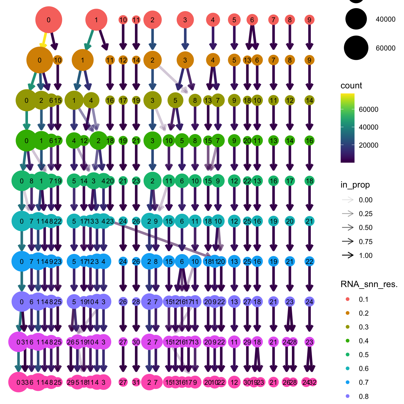
| Version | Author | Date |
|---|---|---|
| b2114c7 | Gunjan Dixit | 2024-12-17 |
Based on the clustering tree, we chose an intermediate/optimum resolution where the clustering results are the most stable, with the least amount of shuffling cells.
opt_res <- "RNA_snn_res.0.4"
n <- nlevels(merged_obj$RNA_snn_res.0.4)
merged_obj$RNA_snn_res.0.4 <- factor(merged_obj$RNA_snn_res.0.4, levels = seq(0,n-1))
merged_obj$seurat_clusters <- NULL
merged_obj$cluster <- merged_obj$RNA_snn_res.0.4
Idents(merged_obj) <- merged_obj$cluster
UMAP after clustering
Defining colours for each cell-type to be consistent with other age-related/cell type composition plots.
my_colors <- c(
  "B cells" = "steelblue",
  "CD4 T cells" = "brown",
  "Double negative T cells" = "gold",
  "CD8 T cells" = "lightgreen",
  "Pre B/T cells" = "orchid",
  "Innate lymphoid cells" = "tan",
  "Natural Killer cells" = "blueviolet",
  "Macrophages" = "green4",
  "Cycling T cells" = "turquoise",
  "Dendritic cells" = "grey80",
  "Gamma delta T cells" = "mediumvioletred",
  "Epithelial lineage" = "darkorange",
  "Granulocytes" = "olivedrab",
  "Fibroblast lineage" = "lavender",
  "None" = "white",
  "Monocytes" = "peachpuff",
  "Endothelial lineage" = "cadetblue",
  "SMG duct" = "lightpink",
  "Neuroendocrine" = "skyblue",
  "Doublet query/Other" = "#d62728"
)
# Define custom colors
custom_colors <- list()
colors_1 <- c(
  '#FFC312', '#C4E538', '#12CBC4', '#FDA7DF', '#ED4C67',
  "lavender", '#A3CB38', '#1289A7', '#D980FA', '#B53471',
  '#EE5A24', '#009432', '#0652DD','#9980FA', "#E5C494",'#833471',
  '#EA2027', '#006266', '#1B1464', '#5758BB', '#6F1E51'
)

colors_2 <- c(
  "darkorange", '#cc8e35', '#ffe119', '#4363d8', '#ffda79',
  '#911eb4', '#42d4f4', '#f032e6', '#bfef45', 'grey90',
  '#469990', '#dcbeff', '#9A6324', '#fffac8', '#800000',
  '#aaffc3', '#808000', '#ffd8b1', '#000075', '#a9a9a9',  "#FB8072"
)

custom_colors$discrete <- c(colors_1, colors_2)
UMAP displaying clusters at opt_res resolution and Broad
cell Labels Level 3.
p1 <- DimPlot(merged_obj, reduction = "umap.harmony", raster = FALSE ,repel = TRUE, label = TRUE,label.size = 3.5, group.by = opt_res) +  NoLegend()

p2 <- DimPlot(merged_obj, reduction = "umap.harmony", raster = FALSE, repel = TRUE, label = TRUE, label.size = 3.5, group.by = "Broad_cell_label_3")  +
  scale_colour_manual(values = my_colors) +
  ggtitle(paste0(tissue, ": Batch Corrected UMAP"))


p1 / p2 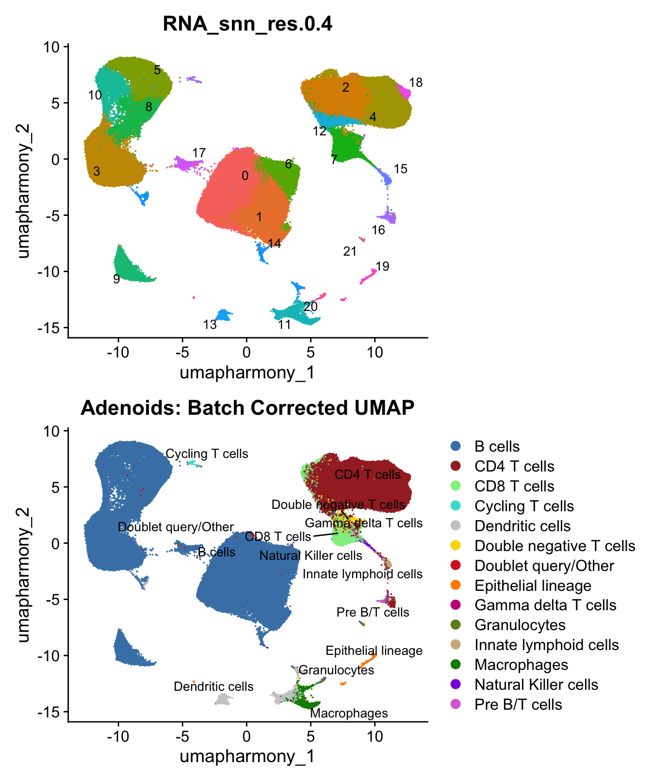
| Version | Author | Date |
|---|---|---|
| b2114c7 | Gunjan Dixit | 2024-12-17 |
p3 <- DimPlot(merged_obj, reduction = "umap.harmony", raster = FALSE, repel = TRUE, label = TRUE, label.size = 3.5, group.by = "predicted.celltype.l1") + NoLegend()
p3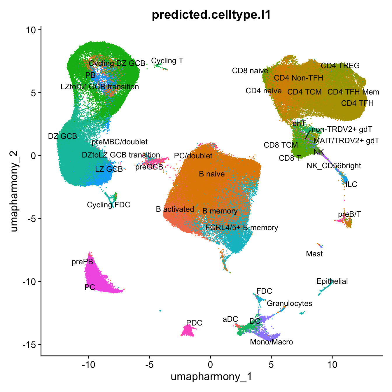
| Version | Author | Date |
|---|---|---|
| b2114c7 | Gunjan Dixit | 2024-12-17 |
p4 <- DimPlot(merged_obj, reduction = "umap.harmony", raster = FALSE, repel = TRUE, label = TRUE, label.size = 3.5, group.by = "predicted.celltype.l2") + NoLegend()
p4
Warning: ggrepel: 46 unlabeled data points (too many overlaps). Consider
increasing max.overlaps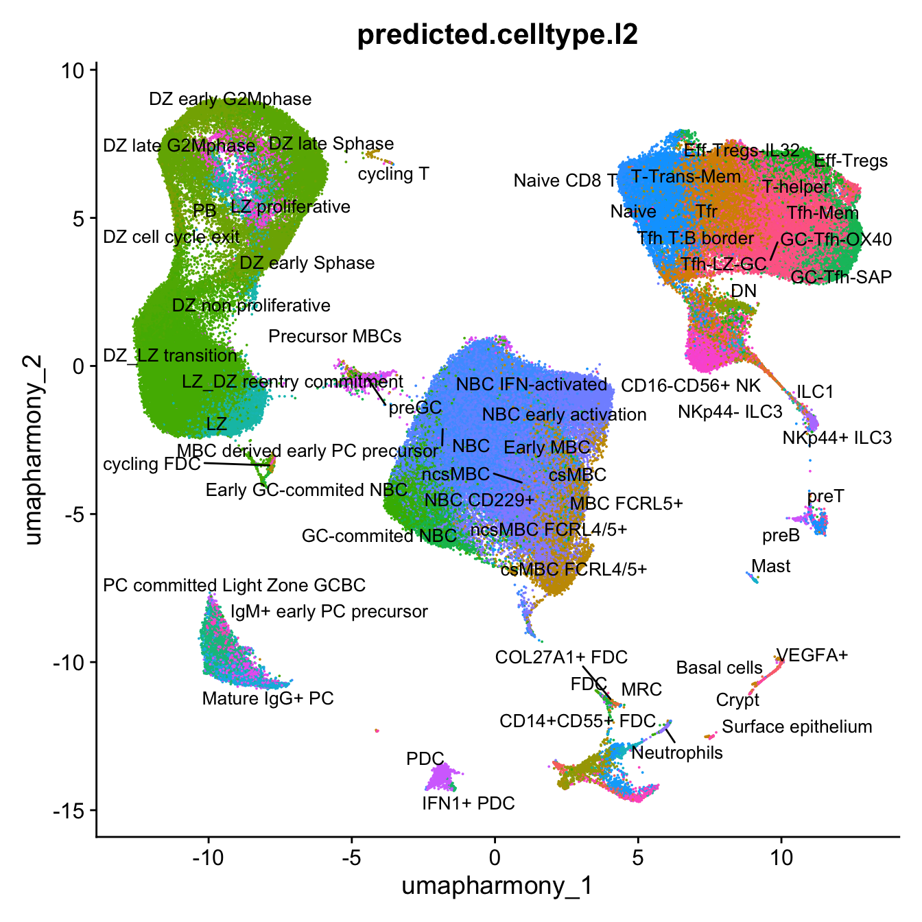
| Version | Author | Date |
|---|---|---|
| b2114c7 | Gunjan Dixit | 2024-12-17 |
p1 <- merged_obj@meta.data %>%
  ggplot(aes(x = !!sym(opt_res),
             fill = !!sym(opt_res))) +
  geom_bar() +
  geom_text(aes(label = ..count..), stat = "count",
            vjust = -0.5, colour = "black", size = 2) +
  scale_y_log10() +
  theme(axis.text.x = element_text(angle = 90,
                                   vjust = 0.5,
                                   hjust = 1,
                                   size = 8)) +
  NoLegend() +
  labs(y = "No. Cells (log scale)")

p2 <- merged_obj@meta.data %>%
  dplyr::select(!!sym(opt_res), predicted.celltype.l1) %>%
  group_by(!!sym(opt_res), predicted.celltype.l1) %>%
  summarise(num = n()) %>%
  mutate(prop = num / sum(num)) %>%
  ggplot(aes(x = !!sym(opt_res), y = prop * 100,
             fill = predicted.celltype.l1)) +
  geom_bar(stat = "identity") +
  theme(axis.text.x = element_text(angle = 90,
                                   vjust = 0.5,
                                   hjust = 1,
                                   size = 8)) +
  labs(y = "% Cells", fill = "predicted.celltype.l1") +
  scale_fill_manual(values = custom_colors$discrete) #+
`summarise()` has grouped output by 'RNA_snn_res.0.4'. You can override using
the `.groups` argument. # paletteer::scale_fill_paletteer_d("ggsci::default_igv")
p3 <- merged_obj@meta.data %>%
dplyr::select(!!sym(opt_res), Broad_cell_label_3) %>%
group_by(!!sym(opt_res), Broad_cell_label_3) %>%
summarise(num = n()) %>%
mutate(prop = num / sum(num)) %>%
ggplot(aes(x = !!sym(opt_res), y = prop * 100,
fill = Broad_cell_label_3)) +
geom_bar(stat = "identity") +
theme(axis.text.x = element_text(angle = 90,
vjust = 0.5,
hjust = 1,
size = 8)) +
labs(y = "% Cells", fill = "Sample") +
scale_fill_manual(values = my_colors) `summarise()` has grouped output by 'RNA_snn_res.0.4'. You can override using
the `.groups` argument.# Combine the plots
(p1 / p2 / p3 ) & theme(legend.text = element_text(size = 8),
legend.key.size = unit(3, "mm"))
| Version | Author | Date |
|---|---|---|
| b2114c7 | Gunjan Dixit | 2024-12-17 |
This table shows Azimuth Level 2 predicted cell types and their counts in each cluster in descending order.
cluster_ids <- sort(unique(merged_obj$cluster))
cluster_celltype_counts <- list()

for (cluster_id in cluster_ids) {
  cluster_data <- merged_obj@meta.data[merged_obj$cluster == cluster_id, ]
  table_counts <- table(cluster_data$predicted.celltype.l2)
  sorted_table <- table_counts[order(-table_counts)]
  cluster_celltype_counts[[as.character(cluster_id)]] <- sorted_table
}

cluster_celltype_counts
$`0`
NBC NBC early activation
17924 17285
Early GC-commited NBC GC-commited NBC
2836 2091
ncsMBC ncsMBC FCRL4/5+
1611 528
NBC IFN-activated Early MBC
522 80
csMBC Precursor MBCs
63 54
MBC FCRL5+ preGC
43 20
DZ_LZ transition csMBC FCRL4/5+
14 12
MBC derived early PC precursor Naive
11 10
CM PreTfh LZ_DZ reentry commitment
5 4
LZ NBC CD229+
2 2
preB DZ non proliferative
2 1
LZ proliferative RM CD8 activated T
1 1
$`1`
ncsMBC ncsMBC FCRL4/5+
6596 5861
NBC csMBC FCRL4/5+
4312 3595
csMBC NBC early activation
3539 1589
MBC FCRL5+ Early MBC
984 233
Early GC-commited NBC GC-commited NBC
195 184
NBC IFN-activated preGC
38 24
Precursor MBCs NBC CD229+
21 6
Naive CM Pre-non-Tfh
5 1
CM PreTfh DZ_LZ transition
1 1
IgM+ early PC precursor MBC derived early PC precursor
1 1
Tfh-LZ-GC
1
$`2`
Naive CM PreTfh
9806 6192
Tfh-LZ-GC CM Pre-non-Tfh
2851 2369
Naive CD8 T Tfh-Mem
1646 649
T-Eff-Mem Eff-Tregs-IL32
601 311
T-Trans-Mem T-helper
283 126
DN Eff-Tregs
84 64
CM CD8 T NBC
36 31
Tfh T:B border NBC early activation
18 17
SCM CD8 T TCRVδ+ gd T
16 14
cycling T preGC
10 9
GC-Tfh-SAP GC-Tfh-OX40
8 7
NKp44+ ILC3 Tfr
6 5
MBC FCRL5+ GC-commited NBC
4 3
ncsMBC csMBC
2 1
IFN+ CD8 T MAIT/CD161+TRDV2+ gd T-cells
1 1
RM CD8 activated T
1
$`3`
DZ_LZ transition DZ non proliferative
17363 3173
LZ LZ_DZ reentry commitment
2086 234
Precursor MBCs PC committed Light Zone GCBC
54 35
preGC DZ cell cycle exit
20 11
IgM+ early PC precursor DZ early Sphase
8 5
Early MBC LZ proliferative
5 3
Mature IgA+ PC GC-commited NBC
3 2
IgM+ PC precursor MBC FCRL5+
1 1
NBC PB
1 1
preMature IgM+ PC Short lived IgM+ PC
1 1
$`4`
Tfh-LZ-GC GC-Tfh-SAP
5813 2852
Tfh-Mem Eff-Tregs
2640 1340
GC-Tfh-OX40 Eff-Tregs-IL32
880 580
T-helper CM PreTfh
468 330
Naive T-Eff-Mem
286 151
CM Pre-non-Tfh T-Trans-Mem
144 63
Naive CD8 T Tfh T:B border
40 17
DN MAIT/CD161+TRDV2+ gd T-cells
12 12
Tfr CD8 Tf
10 5
CM CD8 T NBC
5 5
SCM CD8 T GC-commited NBC
5 3
NKp44+ ILC3 Early GC-commited NBC
3 2
NBC IFN-activated RM CD8 T
2 2
cycling T ILC1
1 1
MBC derived early PC precursor MBC FCRL5+
1 1
NBC early activation preGC
1 1
TCRVδ+ gd T
1
$`5`
DZ late Sphase DZ early G2Mphase
6138 1872
Reactivated proliferative MBCs LZ proliferative
797 319
LZ_DZ transition DZ early Sphase
251 100
DZ late G2Mphase PB
48 34
DZ_LZ transition preGC
23 18
LZ cycling T
10 7
LZ_DZ reentry commitment Precursor MBCs
4 3
Short lived IgM+ PC DZ cell cycle exit
3 1
DZ non proliferative GC-commited NBC
1 1
IgD PC precursor IgM+ PC precursor
1 1
Mature IgA+ PC preMature IgM+ PC
1 1
$`6`
NBC IFN-activated NBC
4305 1350
ncsMBC FCRL4/5+ NBC early activation
488 471
csMBC FCRL4/5+ ncsMBC
269 246
GC-commited NBC csMBC
46 30
Naive Early GC-commited NBC
17 14
MBC FCRL5+ preGC
9 9
Early MBC CM Pre-non-Tfh
4 1
MBC derived early PC precursor Naive CD8 T
1 1
preB preMature IgM+ PC
1 1
Tfh-LZ-GC
1
$`7`
RM CD8 activated T RM CD8 T
1378 1214
DN CM CD8 T
782 617
CD16-CD56+ NK TCRVδ+ gd T
374 362
SCM CD8 T MAIT/CD161+TRDV2+ gd T-cells
258 241
CM Pre-non-Tfh Naive
239 184
IFN+ CD8 T Naive CD8 T
161 159
Eff-Tregs DC recruiters CD8 T
116 101
ZNF683+ CD8 T T-helper
98 77
EM CD8 T CD8 Tf
66 63
CD16-CD56dim NK CD16+CD56- NK
59 56
Tfh-LZ-GC CM PreTfh
51 49
Tfh-Mem Eff-Tregs-IL32
35 32
NBC NKp44+ ILC3
17 11
T-Trans-Mem Tfr
10 9
ILC1 NBC IFN-activated
7 5
NBC early activation GC-Tfh-OX40
4 2
GC-Tfh-SAP preGC
2 2
cycling T GC-commited NBC
1 1
ncsMBC T-Eff-Mem
1 1
$`8`
DZ early Sphase DZ_LZ transition
3542 753
DZ non proliferative Reactivated proliferative MBCs
308 247
LZ proliferative DZ late Sphase
174 126
LZ_DZ reentry commitment LZ
98 76
preGC LZ_DZ transition
45 33
Precursor MBCs DZ cell cycle exit
22 16
DZ late G2Mphase GC-commited NBC
12 2
PB Early MBC
2 1
IgM+ PC precursor Mature IgA+ PC
1 1
MBC derived early PC precursor Naive
1 1
ncsMBC FCRL4/5+
1
$`9`
IgG+ PC precursor preMature IgG+ PC
1856 674
Mature IgG+ PC Mature IgA+ PC
652 402
Short lived IgM+ PC MBC derived IgG+ PC
321 249
MBC derived IgA+ PC IgM+ early PC precursor
204 146
IgM+ PC precursor PC committed Light Zone GCBC
100 76
preMature IgM+ PC PB
75 51
IgD PC precursor Mature IgM+ PC
34 21
csMBC NBC
15 14
PB committed early PC precursor DZ_LZ transition
14 12
MBC derived early PC precursor preGC
10 5
Early PC precursor CM PreTfh
3 1
DZ non proliferative MBC derived PC precursor
1 1
NBC early activation Precursor MBCs
1 1
$`10`
DZ late G2Mphase DZ cell cycle exit
2649 472
Reactivated proliferative MBCs LZ_DZ transition
295 229
DZ_LZ transition DZ non proliferative
168 166
DZ early G2Mphase LZ proliferative
163 155
DZ early Sphase PB
107 30
DZ late Sphase preGC
20 13
LZ Precursor MBCs
7 7
cycling FDC csMBC FCRL4/5+
5 4
IgM+ PC precursor PC committed Light Zone GCBC
4 3
IgG+ PC precursor LZ_DZ reentry commitment
2 2
MBC derived IgA+ PC ncsMBC FCRL4/5+
2 2
cycling T IgM+ early PC precursor
1 1
MBC derived early PC precursor preB
1 1
Proliferative NBC Short lived IgM+ PC
1 1
$`11`
DC2 SELENOP Slan-like MMP Slan-like
639 429 331
Monocytes C1Q Slan-like aDC1
207 158 140
M1 Macrophages DC1 mature DC4
133 120 77
DC1 precursor DC5 ITGAX Slan-like
72 61 42
IL7R DC Crypt Neutrophils
30 8 8
FDC aDC3 DN
3 2 2
Naive Naive CD8 T Tfh-Mem
2 2 2
CD14+CD55+ FDC CM PreTfh Early GC-commited NBC
1 1 1
NBC early activation PDC preB
1 1 1
preGC TCRVδ+ gd T Tfh-LZ-GC
1 1 1
$`12`
CM Pre-non-Tfh Naive Tfh-LZ-GC CM PreTfh
776 501 452 89
Naive CD8 T Tfh-Mem Eff-Tregs NBC IFN-activated
69 38 30 14
GC-Tfh-SAP Eff-Tregs-IL32 NBC T-Eff-Mem
11 9 8 6
IFN+ CD8 T CM CD8 T T-helper DN
5 3 3 2
T-Trans-Mem
2
$`13`
PDC IFN1+ PDC NBC preGC
1447 48 2 1
$`14`
FDC DZ_LZ transition
285 229
NBC ncsMBC FCRL4/5+
124 102
cycling FDC CD14+CD55+ FDC
76 72
ncsMBC csMBC FCRL4/5+
34 33
NBC early activation Reactivated proliferative MBCs
28 24
COL27A1+ FDC NBC IFN-activated
11 10
Tfh-LZ-GC DZ early Sphase
10 9
Early MBC csMBC
8 7
DZ late Sphase LZ
6 6
MRC GC-commited NBC
6 5
MBC FCRL5+ Crypt
5 4
Early GC-commited NBC preGC
3 3
CM PreTfh DC1 mature
2 2
DZ early G2Mphase Naive
2 2
Neutrophils DN
2 1
GC-Tfh-OX40 GC-Tfh-SAP
1 1
IgM+ early PC precursor MAIT/CD161+TRDV2+ gd T-cells
1 1
Naive CD8 T PDC
1 1
Precursor MBCs RM CD8 T
1 1
SELENOP Slan-like T-helper
1 1
TCRVδ+ gd T Tfh-Mem
1 1
$`15`
NKp44+ ILC3 ILC1
667 98
CM Pre-non-Tfh CM PreTfh
42 39
CD16-CD56+ NK T-Trans-Mem
26 20
Naive NBC
11 10
TCRVδ+ gd T CM CD8 T
10 6
T-helper Eff-Tregs
6 3
Eff-Tregs-IL32 Tfh-LZ-GC
3 3
Crypt NBC early activation
2 2
NKp44- ILC3 csMBC FCRL4/5+
2 1
DC5 DN
1 1
MAIT/CD161+TRDV2+ gd T-cells PDC
1 1
preGC preT
1 1
ZNF683+ CD8 T
1
$`16`
Naive cycling T
542 87
preT preB
83 70
Tfh-LZ-GC CM PreTfh
63 22
NBC NBC early activation
14 13
TCRVδ+ gd T Naive CD8 T
13 11
SCM CD8 T Precursor MBCs
11 8
GC-Tfh-OX40 CM Pre-non-Tfh
4 3
GC-Tfh-SAP DN
3 2
DZ late Sphase Eff-Tregs
2 2
NBC IFN-activated T-Eff-Mem
2 2
Early GC-commited NBC LZ_DZ transition
1 1
ncsMBC FCRL4/5+ PDC
1 1
preGC Reactivated proliferative MBCs
1 1
$`17`
preGC csMBC FCRL4/5+
380 145
Early MBC GC-commited NBC
78 29
DZ_LZ transition Precursor MBCs
17 14
ncsMBC FCRL4/5+ NBC
13 8
Reactivated proliferative MBCs csMBC
6 5
Naive NBC IFN-activated
4 4
LZ_DZ reentry commitment MBC FCRL5+
3 2
DZ non proliferative
1
$`18`
Tfh-Mem Tfh-LZ-GC Eff-Tregs GC-Tfh-SAP
209 164 66 45
T-helper Naive CM Pre-non-Tfh GC-Tfh-OX40
28 20 16 16
Eff-Tregs-IL32 cycling T T-Eff-Mem CD8 Tf
13 6 6 3
Naive CD8 T DN CM CD8 T RM CD8 activated T
3 2 1 1
TCRVδ+ gd T
1
$`19`
VEGFA+ Surface epithelium Crypt preGC
198 92 76 9
Basal cells Naive NBC CM Pre-non-Tfh
3 2 2 1
FDC NBC IFN-activated ncsMBC SELENOP Slan-like
1 1 1 1
$`20`
Neutrophils Early GC-commited NBC NBC early activation
234 17 12
Mast NBC GC-commited NBC
11 6 3
Monocytes T-Eff-Mem CM PreTfh
3 3 2
Tfh-LZ-GC Eff-Tregs Eff-Tregs-IL32
2 1 1
FDC ncsMBC FCRL4/5+ preMature IgG+ PC
1 1 1
$`21`
Mast Crypt preGC
148 2 2 Save batch corrected Object
out1 <- here("output",
            "RDS", "AllBatches_Clustering_SEUs_v2",
             paste0("G000231_Neeland_",tissue,".Clusters.SEU.rds"))
#dir.create(out1)
if (!file.exists(out1)) {
  saveRDS(merged_obj, file = out1)
}
Marker Gene Analysis
The marker genes for this reclustering can be found here-
merged_obj <- JoinLayers(merged_obj)
paed.markers <- FindAllMarkers(merged_obj, only.pos = TRUE, min.pct = 0.25, logfc.threshold = 0.25)
Extracting top 5 genes per cluster for visualization. The ‘top5’ contains the top 5 genes with the highest weighted average avg_log2FC within each cluster and the ‘best.wilcox.gene.per.cluster’ contains the single best gene with the highest weighted average avg_log2FC for each cluster.
paed.markers %>%
    group_by(cluster) %>% unique() %>%
    top_n(n = 5, wt = avg_log2FC) -> top5

paed.markers %>%
    group_by(cluster) %>%
    slice_head(n=1) %>%
    pull(gene) -> best.wilcox.gene.per.cluster

best.wilcox.gene.per.cluster
[1] "IGHD" "TNFRSF13B" "TCF7" "MEF2B" "MAF" "TYMS"
[7] "IFI44L" "CCL5" "MCM4" "MZB1" "CCNB2" "LYZ"
[13] "IFI44L" "CLEC4C" "CLU" "KIT" "RAG1" "ACTB"
[19] "MAF" "ELF3" "G0S2" "CPA3" Marker gene expression in clusters
This heatmap depicts the expression of top five genes in each cluster.
DoHeatmap(merged_obj, features = top5$gene) + NoLegend()
| Version | Author | Date |
|---|---|---|
| b2114c7 | Gunjan Dixit | 2024-12-17 |
Violin plot shows the expression of top marker gene per cluster.
VlnPlot(merged_obj, features=best.wilcox.gene.per.cluster, ncol = 2, raster = FALSE, pt.size = FALSE)
| Version | Author | Date |
|---|---|---|
| b2114c7 | Gunjan Dixit | 2024-12-17 |
Violin plot shows the expression of top marker gene per cluster and compares its expression in both batches.
plots <- VlnPlot(merged_obj, features = best.wilcox.gene.per.cluster, split.by = "batch_name", group.by = "Broad_cell_label_3",
    pt.size = 0, combine = FALSE, raster = FALSE, split.plot = TRUE)
The default behaviour of split.by has changed.
Separate violin plots are now plotted side-by-side.
To restore the old behaviour of a single split violin,
set split.plot = TRUE.
This message will be shown once per session.wrap_plots(plots = plots, ncol = 1)
| Version | Author | Date |
|---|---|---|
| b2114c7 | Gunjan Dixit | 2024-12-17 |
Feature plot shows the expression of top marker genes per cluster.
FeaturePlot(merged_obj,features=best.wilcox.gene.per.cluster, reduction = 'umap.harmony', raster = FALSE, ncol = 2)
| Version | Author | Date |
|---|---|---|
| b2114c7 | Gunjan Dixit | 2024-12-17 |
Extract markers for each cluster
This section extracts marker genes for each cluster and save them as a CSV file.
out_markers <- here("output",
            "CSV_v2", tissue,
            paste(tissue,"_Marker_gene_clusters.",opt_res, sep = ""))

dir.create(out_markers, recursive = TRUE, showWarnings = FALSE)

for (cl in unique(paed.markers$cluster)) {
  cluster_data <- paed.markers %>% dplyr::filter(cluster == cl)
  file_name <- here(out_markers, paste0("G000231_Neeland_",tissue, "_cluster_", cl, ".csv"))
  write.csv(cluster_data, file = file_name)
}
merged_obj@meta.data %>%
ggplot(aes(x = cell_labels, fill = cell_labels)) +
geom_bar() +
geom_text(aes(label = ..count..), stat = "count",
vjust = -0.5, colour = "black", size = 2) +
theme(axis.text.x = element_text(angle = 90, vjust = 0.5, hjust = 1)) +
NoLegend() + ggtitle(paste0(tissue, " : Counts per cell-type"))Updated cell-type labels (all clusters)
cell_labels <- readxl::read_excel(here("data/cell_labels_Mel_v4_Dec2024/earlyAIR_Adenoids_all.xlsx"), sheet = "all_clusters")

new_cluster_names <- cell_labels %>%
  dplyr::select(cluster, annotation) %>%
  deframe()

merged_obj <- RenameIdents(merged_obj, new_cluster_names)
merged_obj@meta.data$cell_labels <- Idents(merged_obj)

p3 <- DimPlot(merged_obj, reduction = "umap.harmony", raster = FALSE, repel = TRUE, label = TRUE, label.size = 3.5) + ggtitle(paste0(tissue, ": UMAP with Updated cell types"))

p3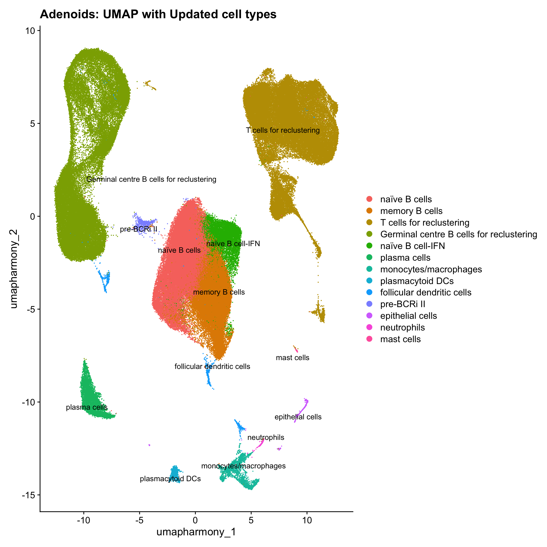
| Version | Author | Date |
|---|---|---|
| 54e4ec2 | Gunjan Dixit | 2025-01-08 |
Summary plots
palette1 <- paletteer::paletteer_d("ggthemes::Classic_20")
palette2 <- paletteer::paletteer_d("Polychrome::light")
combined_palette <- unique(c(palette1, palette2))

labels <- c("cell_labels")

p <- vector("list",length(labels))
for(label in labels){
  merged_obj@meta.data %>%
    ggplot(aes(x = !!sym(label),
               fill = !!sym(label))) +
    geom_bar() +
    geom_text(aes(label = ..count..), stat = "count",
              vjust = -0.5, colour = "black", size = 2) +
    scale_y_log10() +
    theme(axis.text.x = element_blank(),
          axis.title.x = element_blank(),
          axis.ticks.x = element_blank()) +
    NoLegend() +
    labs(y = "No. Cells (log scale)") -> p1

  merged_obj@meta.data %>%
    dplyr::select(!!sym(label), donor_id) %>%
    group_by(!!sym(label), donor_id) %>%
    summarise(num = n()) %>%
    mutate(prop = num / sum(num)) %>%
  ggplot(aes(x = !!sym(label), y = prop * 100,
             fill = donor_id)) +
    geom_bar(stat = "identity") +
    theme(axis.text.x = element_text(angle = 90,
                                     vjust = 0.5,
                                     hjust = 1,
                                     size = 8)) +
    labs(y = "% Cells", fill = "Donor") +
  scale_fill_manual(values = combined_palette) -> p2

  (p1 / p2) & theme(legend.text = element_text(size = 8),
                  legend.key.size = unit(3, "mm")) -> p[[label]]
}
`summarise()` has grouped output by 'cell_labels'. You can override using the
`.groups` argument.p[[1]]
NULL
$cell_labels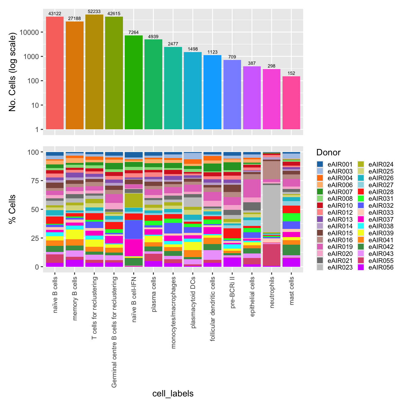
| Version | Author | Date |
|---|---|---|
| 54e4ec2 | Gunjan Dixit | 2025-01-08 |
Reclustering T cell subsets
Reclustering clusters
The marker genes for this reclustering can be found here-
Adenoids_Tcell_population_res.0.4
#sub_clusters <- c(2,4,7,12,15,16,18)

#idx <- which(merged_obj$cluster %in% sub_clusters)
idx <- which(Idents(merged_obj) %in% "T cells for reclustering")
paed_sub <- merged_obj[,idx]
paed_sub
An object of class Seurat
17456 features across 52233 samples within 1 assay
Active assay: RNA (17456 features, 2000 variable features)
3 layers present: data, counts, scale.data
4 dimensional reductions calculated: pca, umap.unintegrated, harmony, umap.harmony# Visualize the clustering results
DimPlot(paed_sub, reduction = "umap.harmony", group.by = "cluster", label = TRUE, label.size = 2.5, repel = TRUE, raster = FALSE )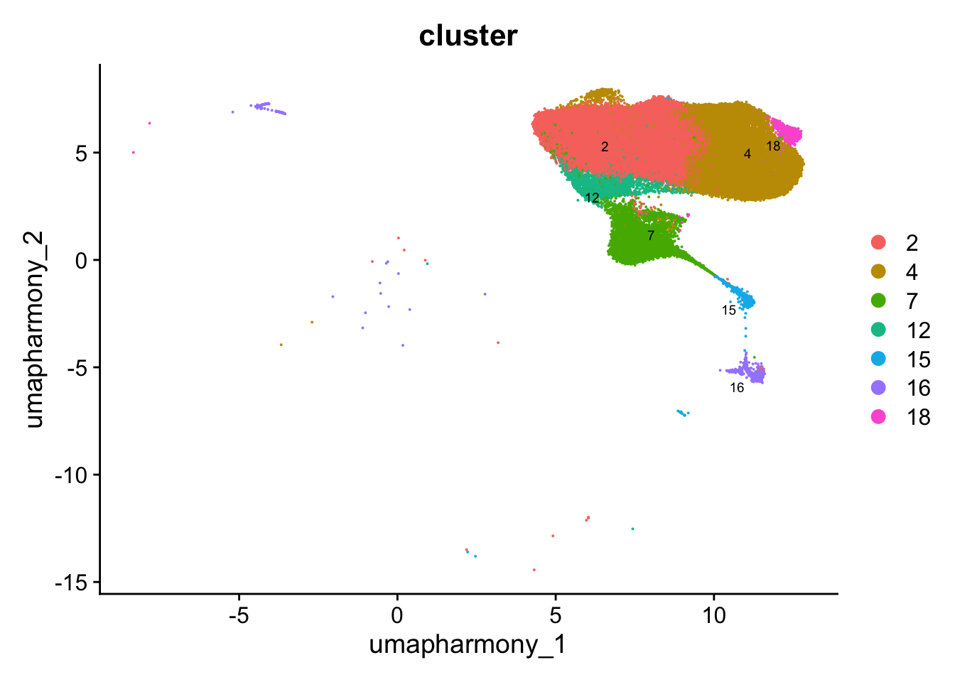
| Version | Author | Date |
|---|---|---|
| b2114c7 | Gunjan Dixit | 2024-12-17 |
paed_sub <- paed_sub %>%
  NormalizeData() %>%
  FindVariableFeatures() %>%
  ScaleData() %>%
  RunPCA()

paed_sub <- RunUMAP(paed_sub, dims = 1:30, reduction = "pca", reduction.name = "umap.tcell")
meta_data_columns <- colnames(paed_sub@meta.data)
columns_to_remove <- grep("^RNA_snn_res", meta_data_columns, value = TRUE)
paed_sub@meta.data <- paed_sub@meta.data[, !(colnames(paed_sub@meta.data) %in% columns_to_remove)]resolutions <- seq(0.1, 1, by = 0.1)
paed_sub <- FindNeighbors(paed_sub, dims = 1:30, reduction = "pca")
paed_sub <- FindClusters(paed_sub, resolution = resolutions )Modularity Optimizer version 1.3.0 by Ludo Waltman and Nees Jan van Eck
Number of nodes: 52233
Number of edges: 1605362
Running Louvain algorithm...
Maximum modularity in 10 random starts: 0.9549
Number of communities: 9
Elapsed time: 8 seconds
Modularity Optimizer version 1.3.0 by Ludo Waltman and Nees Jan van Eck
Number of nodes: 52233
Number of edges: 1605362
Running Louvain algorithm...
Maximum modularity in 10 random starts: 0.9376
Number of communities: 13
Elapsed time: 11 seconds
Modularity Optimizer version 1.3.0 by Ludo Waltman and Nees Jan van Eck
Number of nodes: 52233
Number of edges: 1605362
Running Louvain algorithm...
Maximum modularity in 10 random starts: 0.9262
Number of communities: 14
Elapsed time: 7 seconds
Modularity Optimizer version 1.3.0 by Ludo Waltman and Nees Jan van Eck
Number of nodes: 52233
Number of edges: 1605362
Running Louvain algorithm...
Maximum modularity in 10 random starts: 0.9154
Number of communities: 15
Elapsed time: 7 seconds
Modularity Optimizer version 1.3.0 by Ludo Waltman and Nees Jan van Eck
Number of nodes: 52233
Number of edges: 1605362
Running Louvain algorithm...
Maximum modularity in 10 random starts: 0.9063
Number of communities: 19
Elapsed time: 7 seconds
Modularity Optimizer version 1.3.0 by Ludo Waltman and Nees Jan van Eck
Number of nodes: 52233
Number of edges: 1605362
Running Louvain algorithm...
Maximum modularity in 10 random starts: 0.8977
Number of communities: 21
Elapsed time: 9 seconds
Modularity Optimizer version 1.3.0 by Ludo Waltman and Nees Jan van Eck
Number of nodes: 52233
Number of edges: 1605362
Running Louvain algorithm...
Maximum modularity in 10 random starts: 0.8895
Number of communities: 24
Elapsed time: 8 seconds
Modularity Optimizer version 1.3.0 by Ludo Waltman and Nees Jan van Eck
Number of nodes: 52233
Number of edges: 1605362
Running Louvain algorithm...
Maximum modularity in 10 random starts: 0.8829
Number of communities: 25
Elapsed time: 7 seconds
Modularity Optimizer version 1.3.0 by Ludo Waltman and Nees Jan van Eck
Number of nodes: 52233
Number of edges: 1605362
Running Louvain algorithm...
Maximum modularity in 10 random starts: 0.8764
Number of communities: 26
Elapsed time: 8 seconds
Modularity Optimizer version 1.3.0 by Ludo Waltman and Nees Jan van Eck
Number of nodes: 52233
Number of edges: 1605362
Running Louvain algorithm...
Maximum modularity in 10 random starts: 0.8698
Number of communities: 26
Elapsed time: 7 secondsclustree(paed_sub, prefix = "RNA_snn_res.")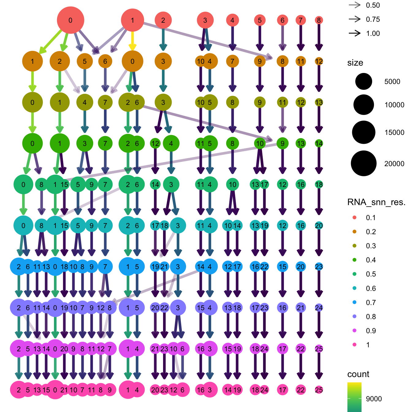
| Version | Author | Date |
|---|---|---|
| b2114c7 | Gunjan Dixit | 2024-12-17 |
# Visualize the clustering results
DimPlot(paed_sub, group.by = "RNA_snn_res.0.4", reduction = "umap.tcell", label = TRUE, label.size = 2.5, repel = TRUE, raster = FALSE )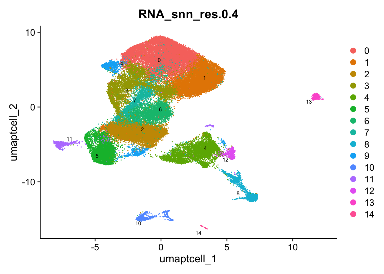
opt_res <- "RNA_snn_res.0.4"
n <- nlevels(paed_sub$RNA_snn_res.0.4)
paed_sub$RNA_snn_res.0.4 <- factor(paed_sub$RNA_snn_res.0.4, levels = seq(0,n-1))
paed_sub$seurat_clusters <- NULL
paed_sub$cluster <- paed_sub$RNA_snn_res.0.4
Idents(paed_sub) <- paed_sub$cluster
paed_sub.markers <- FindAllMarkers(paed_sub, only.pos = TRUE, min.pct = 0.25, logfc.threshold = 0.25)Calculating cluster 0Calculating cluster 1Calculating cluster 2Calculating cluster 3Calculating cluster 4Calculating cluster 5Calculating cluster 6Calculating cluster 7Calculating cluster 8Calculating cluster 9Calculating cluster 10Calculating cluster 11Calculating cluster 12Calculating cluster 13Calculating cluster 14paed_sub.markers %>%
group_by(cluster) %>% unique() %>%
top_n(n = 5, wt = avg_log2FC) -> top5
paed_sub.markers %>%
group_by(cluster) %>%
slice_head(n=1) %>%
pull(gene) -> best.wilcox.gene.per.cluster
best.wilcox.gene.per.cluster [1] "PDCD1" "CD40LG" "KLF2" "CTLA4" "CCL5" "CD8A" "KLF2" "IFI44L"
[9] "TRDC" "STMN1" "CD1E" "GZMK" "CCL5" "MS4A1" "CD24" Violin plot shows the expression of top marker gene per cluster.
VlnPlot(paed_sub, features=best.wilcox.gene.per.cluster, ncol = 2, raster = FALSE, pt.size = FALSE)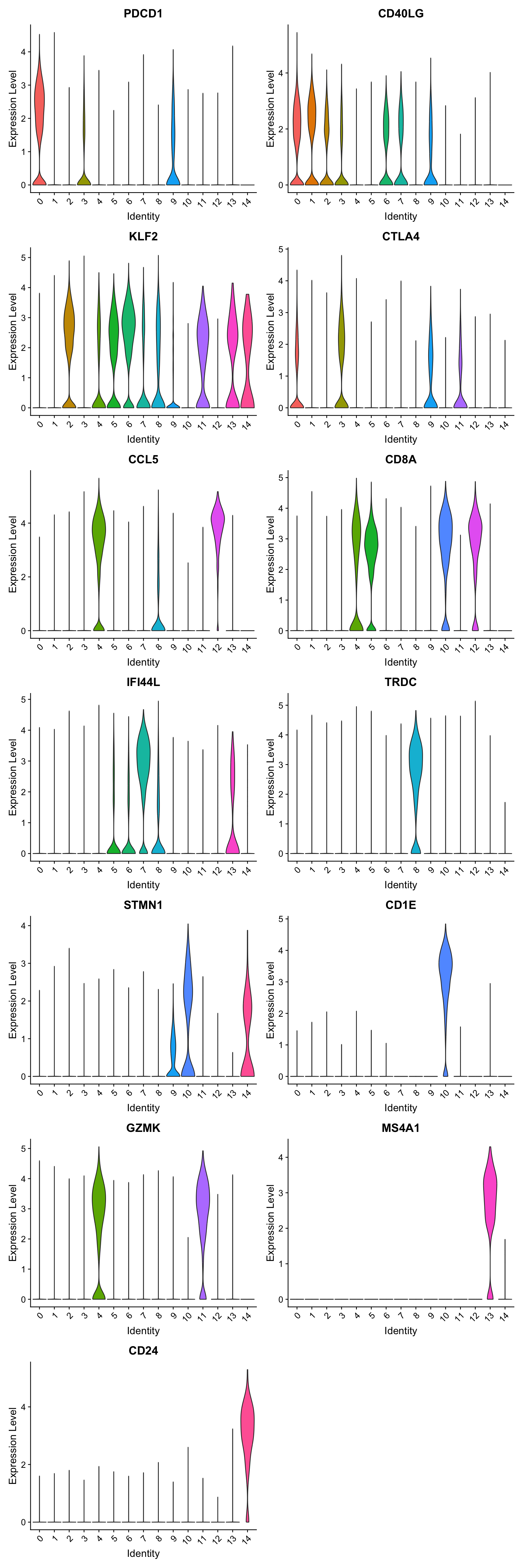
| Version | Author | Date |
|---|---|---|
| b2114c7 | Gunjan Dixit | 2024-12-17 |
Feature plot shows the expression of top marker genes per cluster.
FeaturePlot(paed_sub,features=best.wilcox.gene.per.cluster, reduction = 'umap.tcell', raster = FALSE, ncol = 3, label = TRUE)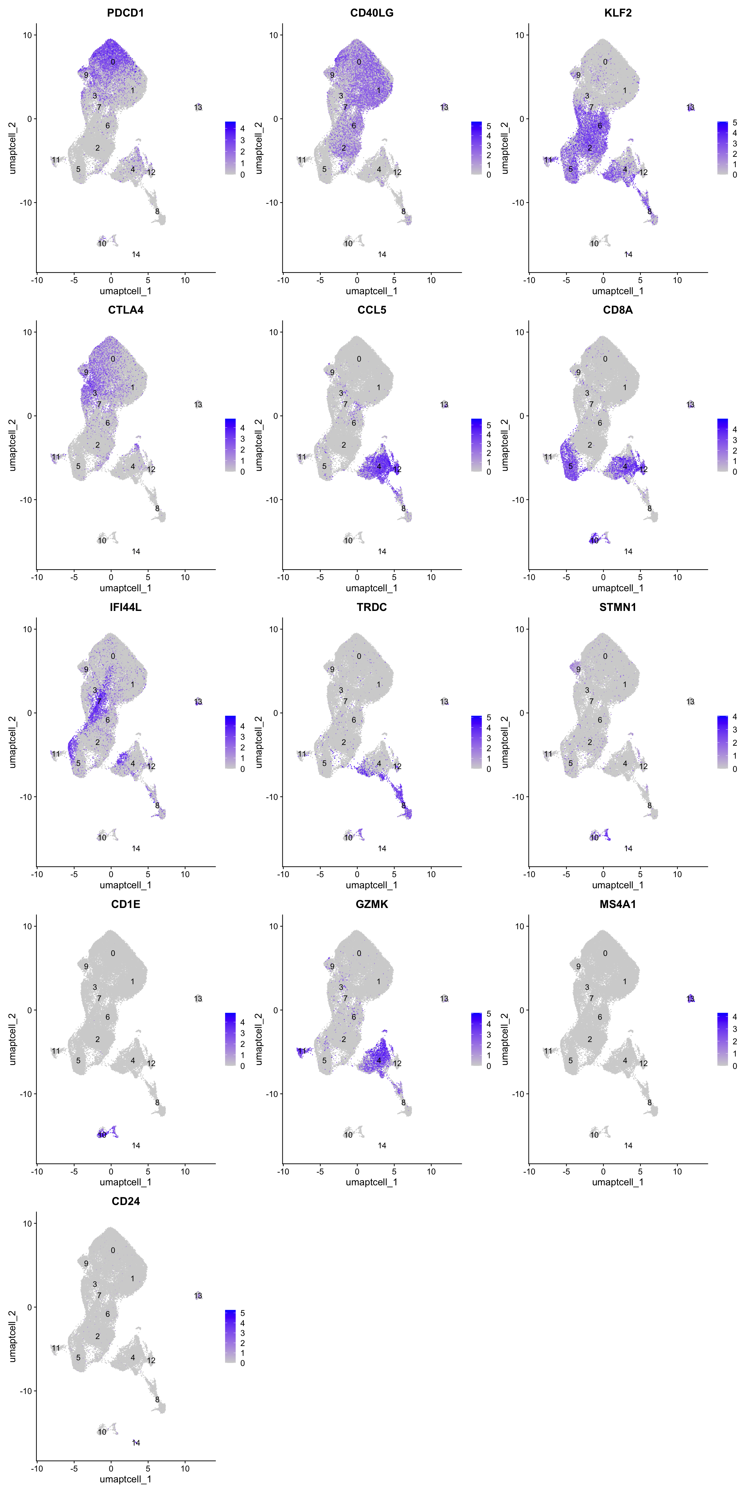
Top 10 marker genes from Seurat
## Seurat top markers
top10 <- paed_sub.markers %>%
    group_by(cluster) %>%
    top_n(n = 10, wt = avg_log2FC) %>%
    ungroup() %>%
    distinct(gene, .keep_all = TRUE) %>%
    arrange(cluster, desc(avg_log2FC))

cluster_colors <- paletteer::paletteer_d("pals::glasbey")[factor(top10$cluster)]

DotPlot(paed_sub,
        features = unique(top10$gene),
        group.by = opt_res,
        cols = c("azure1", "blueviolet"),
        dot.scale = 3, assay = "RNA") +
    RotatedAxis() +
    FontSize(y.text = 8, x.text = 12) +
    labs(y = element_blank(), x = element_blank()) +
    coord_flip() +
    theme(axis.text.y = element_text(color = cluster_colors)) +
    ggtitle("Top 10 marker genes per cluster (Seurat)")
Warning: Vectorized input to `element_text()` is not officially supported.
ℹ Results may be unexpected or may change in future versions of ggplot2.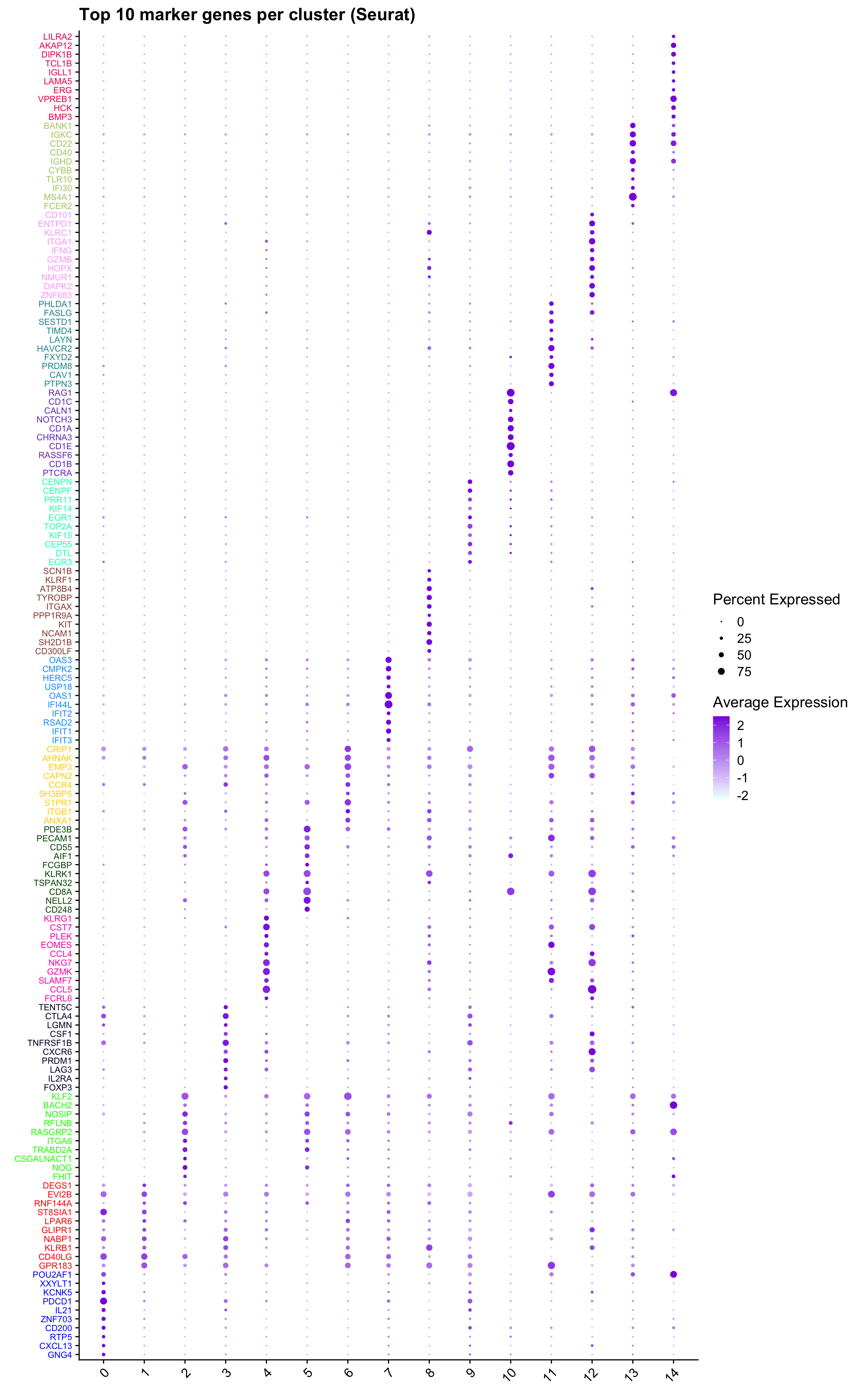
| Version | Author | Date |
|---|---|---|
| 54e4ec2 | Gunjan Dixit | 2025-01-08 |
palette1 <- paletteer::paletteer_d("ggthemes::Classic_20")
palette2 <- paletteer::paletteer_d("Polychrome::light")
combined_palette <- unique(c(palette1, palette2))

labels <- "RNA_snn_res.0.4"

p <- vector("list",length(labels))
for(label in labels){
  paed_sub@meta.data %>%
    ggplot(aes(x = !!sym(label),
               fill = !!sym(label))) +
    geom_bar() +
    geom_text(aes(label = ..count..), stat = "count",
              vjust = -0.5, colour = "black", size = 2) +
    scale_y_log10() +
    theme(axis.text.x = element_blank(),
          axis.title.x = element_blank(),
          axis.ticks.x = element_blank()) +
    NoLegend() +
    labs(y = "No. Cells (log scale)") -> p1

  paed_sub@meta.data %>%
    dplyr::select(!!sym(label), donor_id) %>%
    group_by(!!sym(label), donor_id) %>%
    summarise(num = n()) %>%
    mutate(prop = num / sum(num)) %>%
  ggplot(aes(x = !!sym(label), y = prop * 100,
             fill = donor_id)) +
    geom_bar(stat = "identity") +
    theme(axis.text.x = element_text(angle = 90,
                                     vjust = 0.5,
                                     hjust = 1,
                                     size = 8)) +
    labs(y = "% Cells", fill = "Donor") +
  scale_fill_manual(values = combined_palette) -> p2

  (p1 / p2) & theme(legend.text = element_text(size = 8),
                  legend.key.size = unit(3, "mm")) -> p[[label]]
}
`summarise()` has grouped output by 'RNA_snn_res.0.4'. You can override using
the `.groups` argument.p[[1]]
NULL
$RNA_snn_res.0.4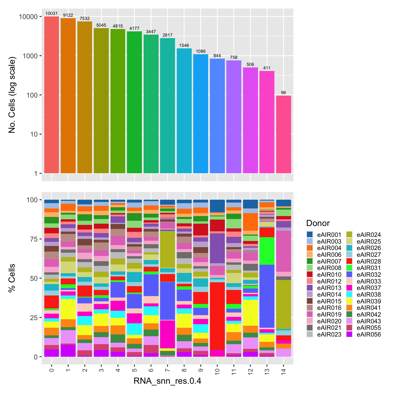
out_markers <- here("output",
            "CSV_v2", tissue,
            paste(tissue,"_Marker_genes_Reclustered_Tcell_population.",opt_res, sep = ""))

dir.create(out_markers, recursive = TRUE, showWarnings = FALSE)

for (cl in unique(paed_sub.markers$cluster)) {
  cluster_data <- paed_sub.markers %>% dplyr::filter(cluster == cl)
  file_name <- here(out_markers, paste0("G000231_Neeland_",tissue, "_cluster_", cl, ".csv"))
  if (!file.exists(file_name)) {
  write.csv(cluster_data, file = file_name)
  }
}
Corresponding Azimuth labels (T cell subsets)
## Level 1
DimPlot(paed_sub, reduction = "umap.tcell", group.by = "predicted.celltype.l1", raster = FALSE, repel = TRUE, label = TRUE, label.size = 4.5)
Warning: ggrepel: 1 unlabeled data points (too many overlaps). Consider
increasing max.overlaps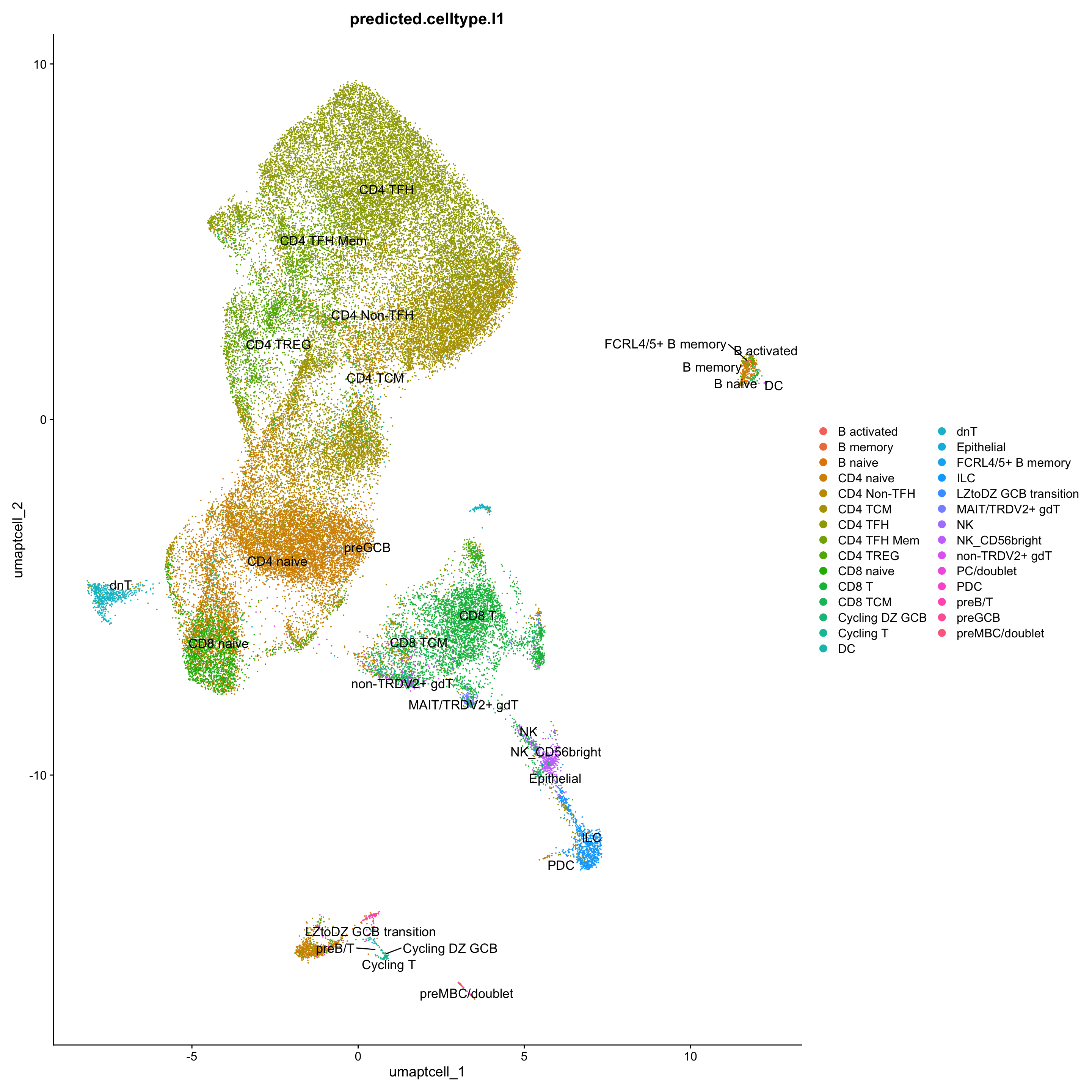
| Version | Author | Date |
|---|---|---|
| 54e4ec2 | Gunjan Dixit | 2025-01-08 |
sort(table(paed_sub$predicted.celltype.l1), decreasing = T)
              CD4 TFH               CD4 TCM             CD4 naive
                14070                 10632                 10625
                CD8 T              CD4 TREG           CD4 TFH Mem
                 3464                  2909                  2730
          CD4 Non-TFH             CD8 naive               CD8 TCM
                 1874                  1835                  1111
                  ILC                   dnT         NK_CD56bright
                  834                   820                   361
       non-TRDV2+ gdT       MAIT/TRDV2+ gdT               B naive
                  231                   172                   161
               preB/T                    NK             Cycling T
                  150                   111                   100
               preGCB           B activated              B memory
                   10                     7                     7
       preMBC/doublet            Epithelial     FCRL4/5+ B memory
                    7                     3                     3
       Cycling DZ GCB                    DC LZtoDZ GCB transition
                    2                     1                     1
           PC/doublet                   PDC
                    1                     1
# Plots for Level 1
DimPlot(paed_sub, reduction = "umap.tcell", group.by = "predicted.celltype.l1", raster = FALSE, repel = TRUE, label = TRUE, label.size = 5) +
paletteer::scale_colour_paletteer_d("Polychrome::palette36")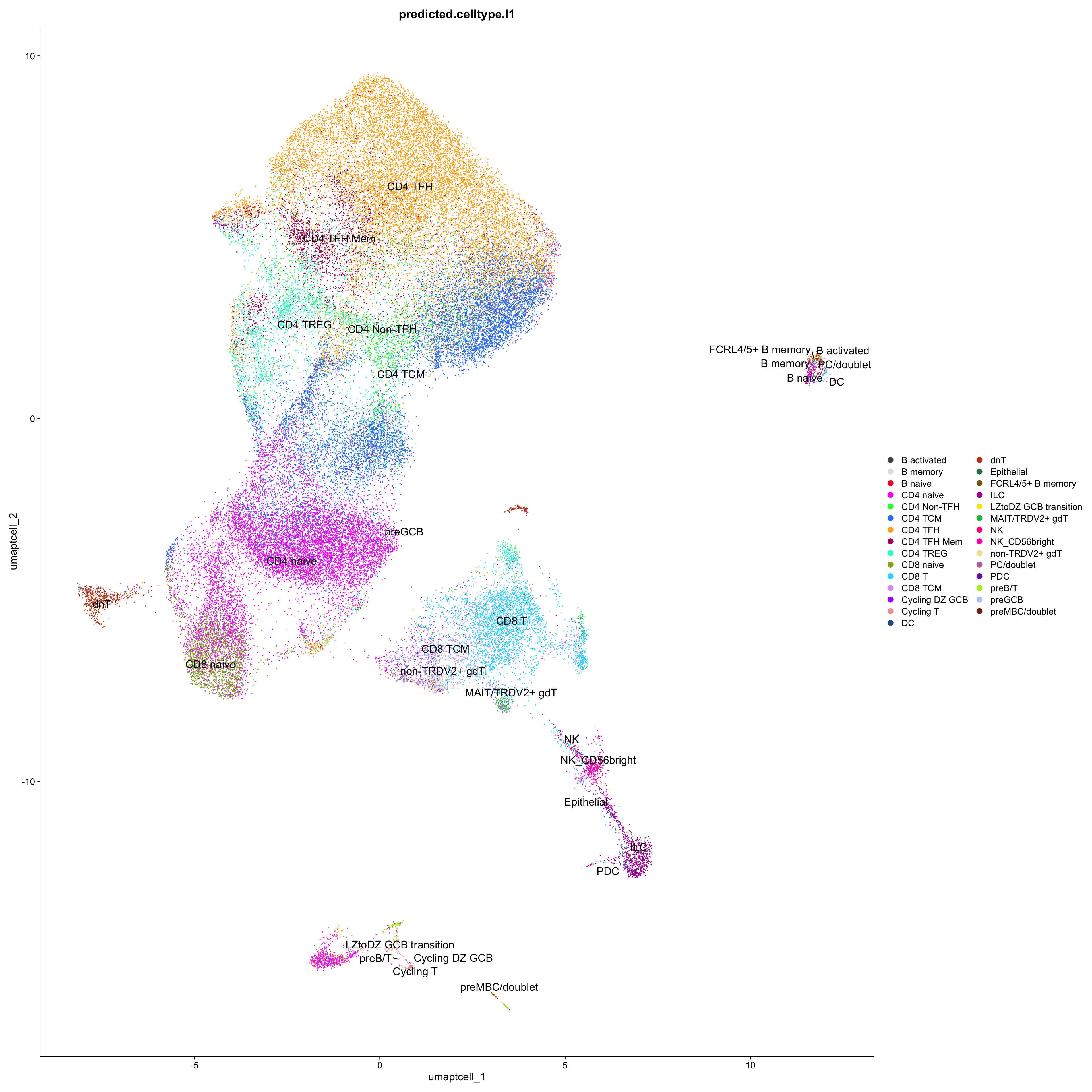
df_table_l1 <- as.data.frame(table(paed_sub$RNA_snn_res.0.4, paed_sub$predicted.celltype.l1))

ggplot(df_table_l1, aes(Var1, Freq, fill = Var2)) +
  geom_bar(stat = "identity") +
  labs(x = "RNA_snn_res.0.4", y = "Count", fill = "predicted.celltype.l1") +
  theme_minimal() +
  paletteer::scale_fill_paletteer_d("Polychrome::palette36") +
  ggtitle("Stacked Bar Plot of Tcell subsets (res=0.4) and predicted.celltype.l1")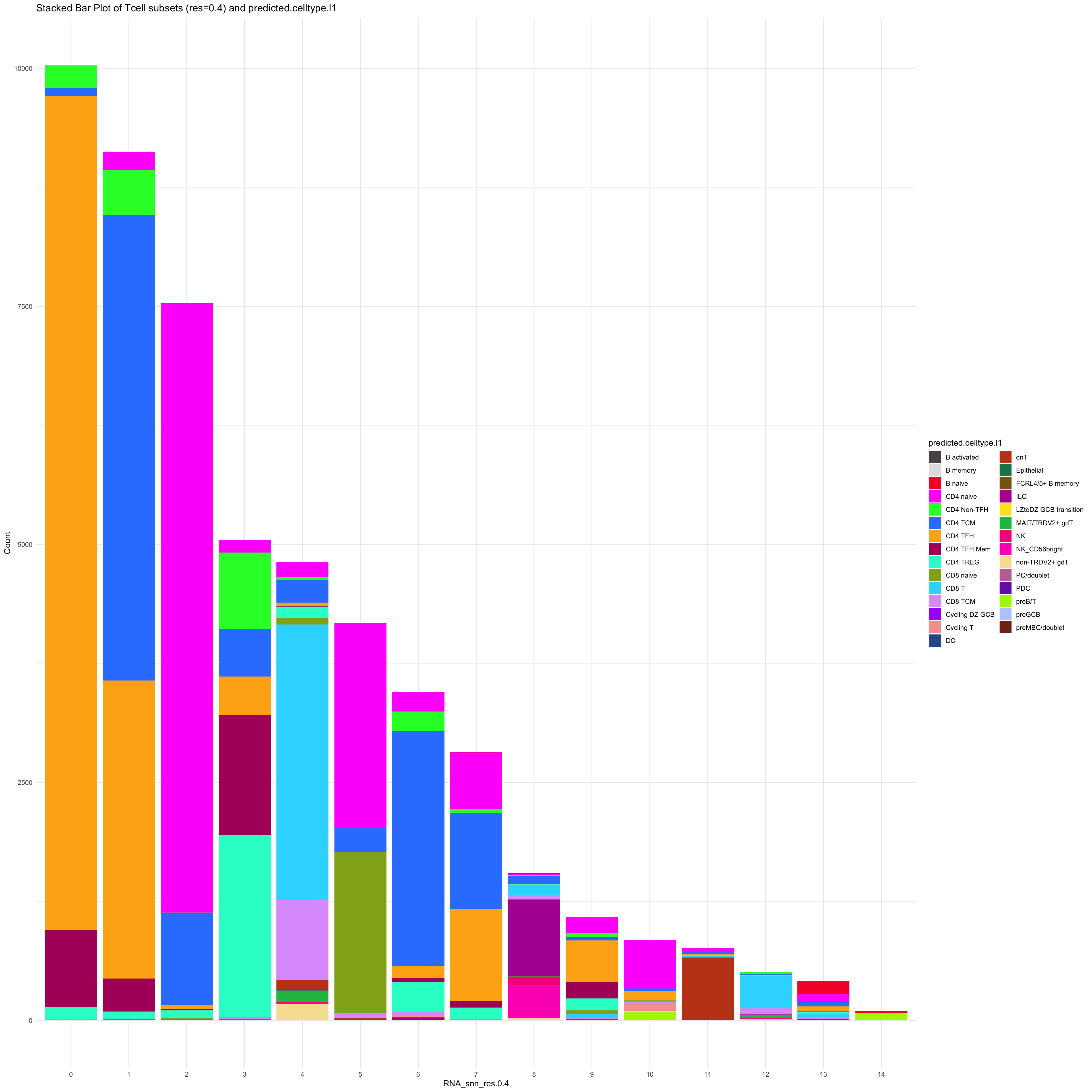
Old data- cells from previous clusters higlighted
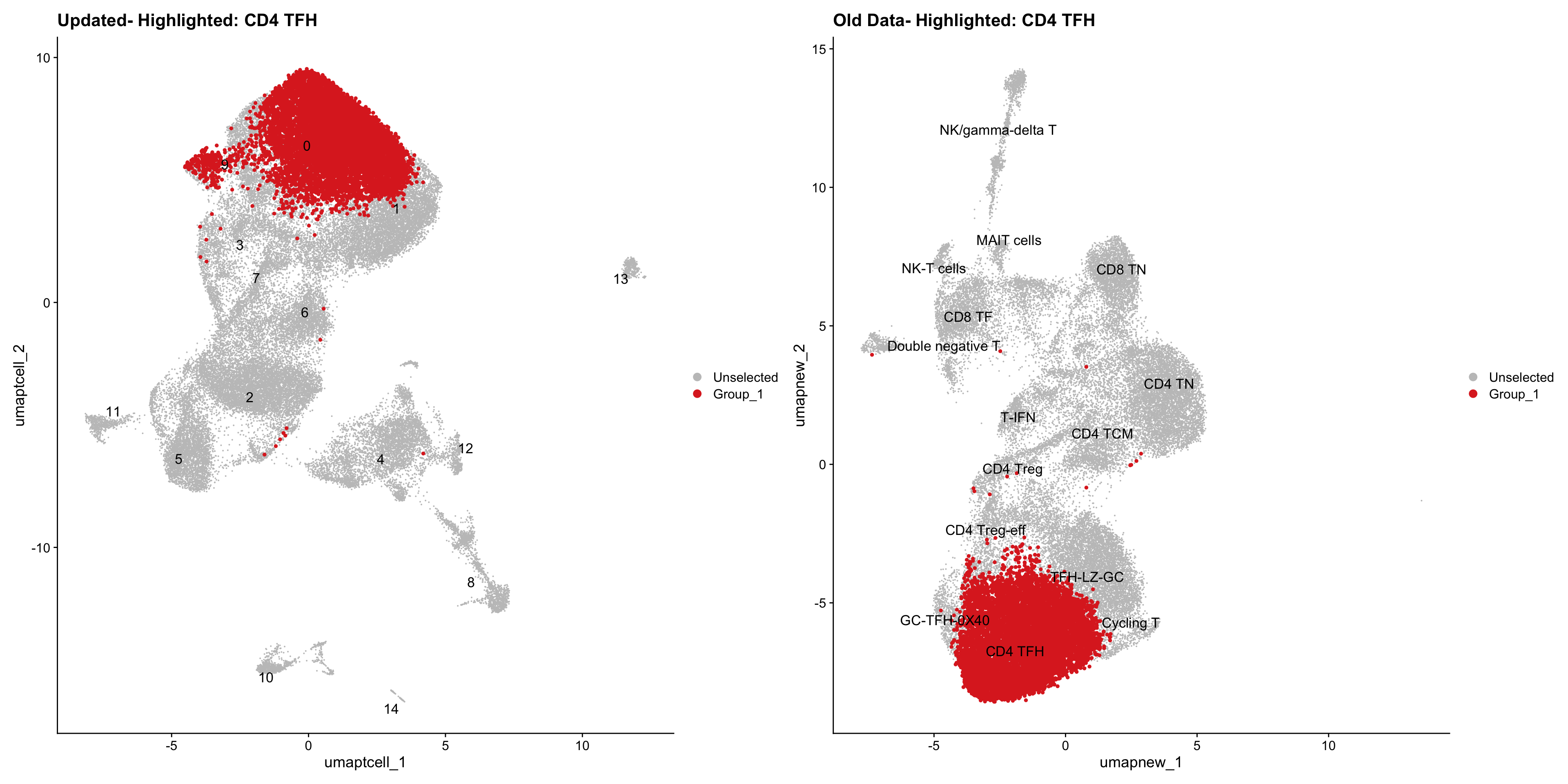
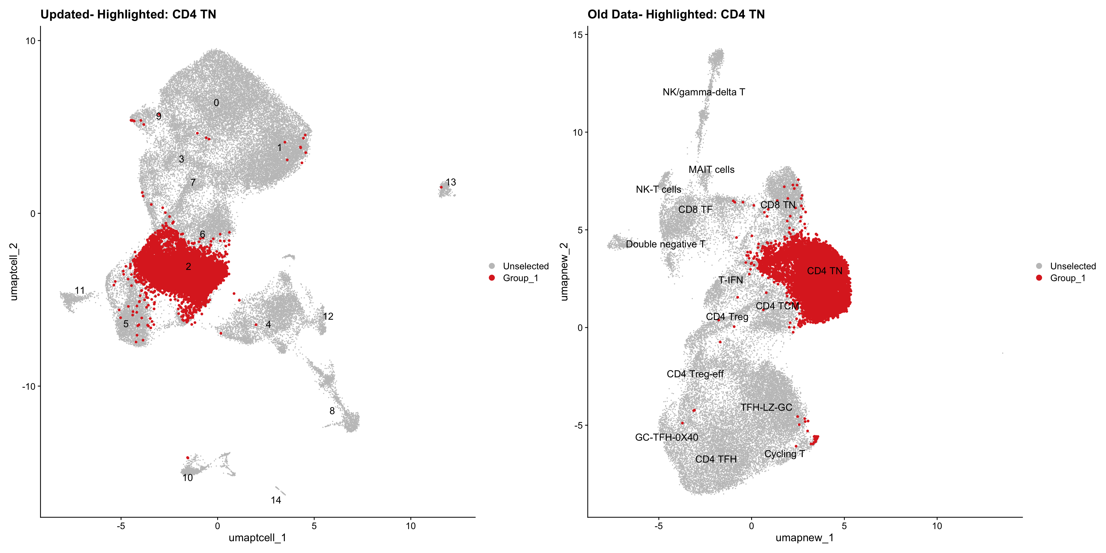
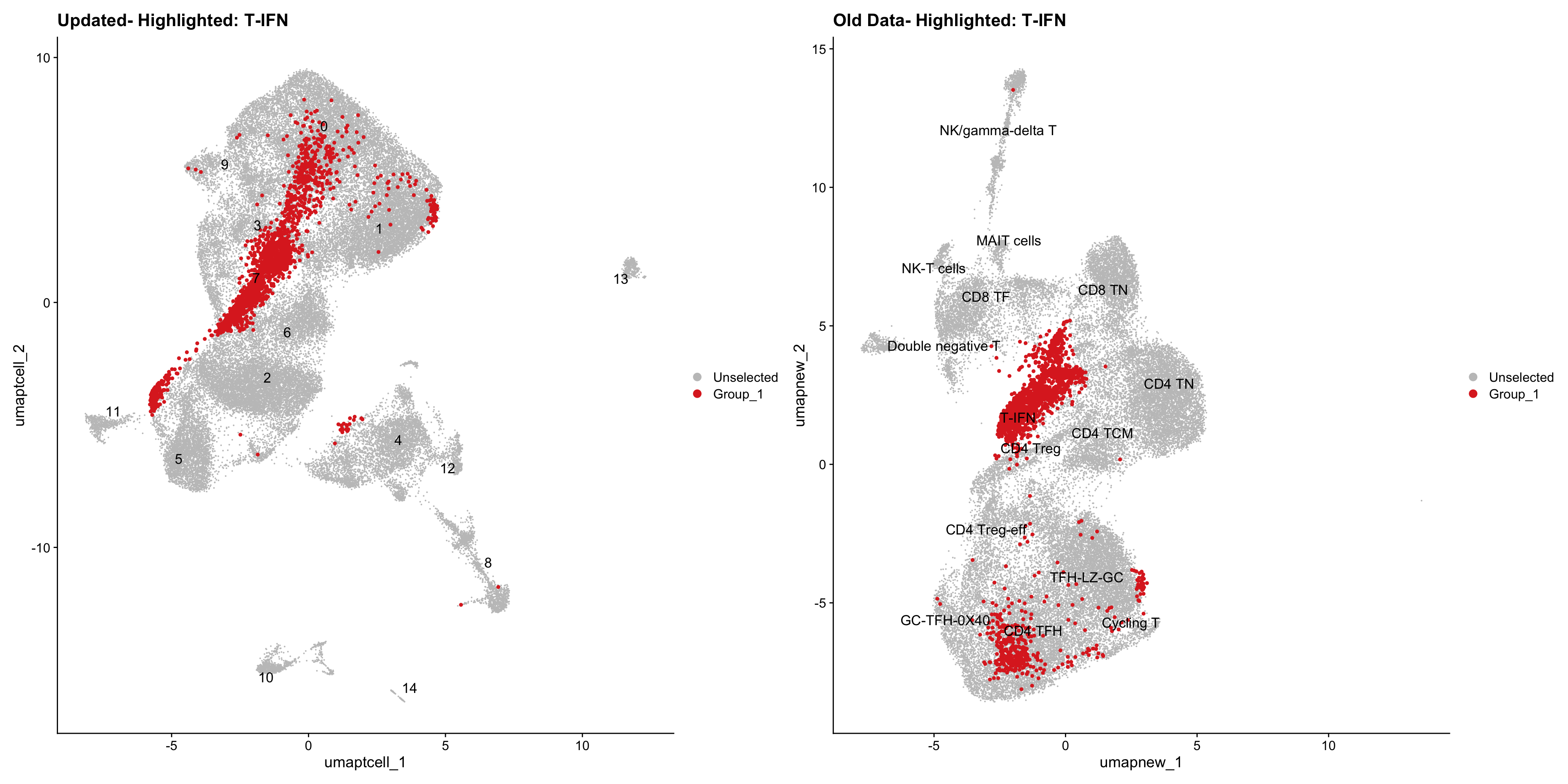
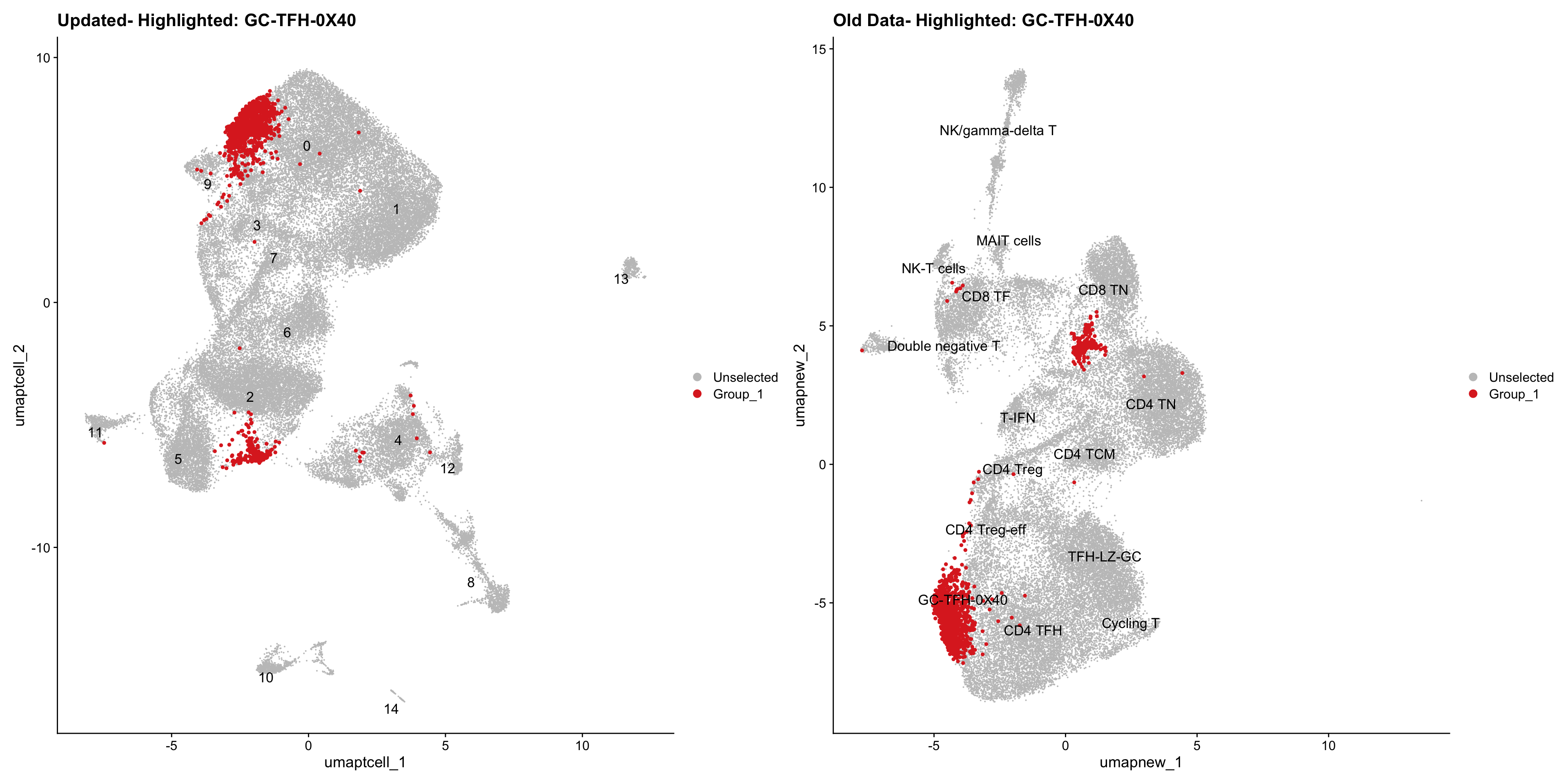
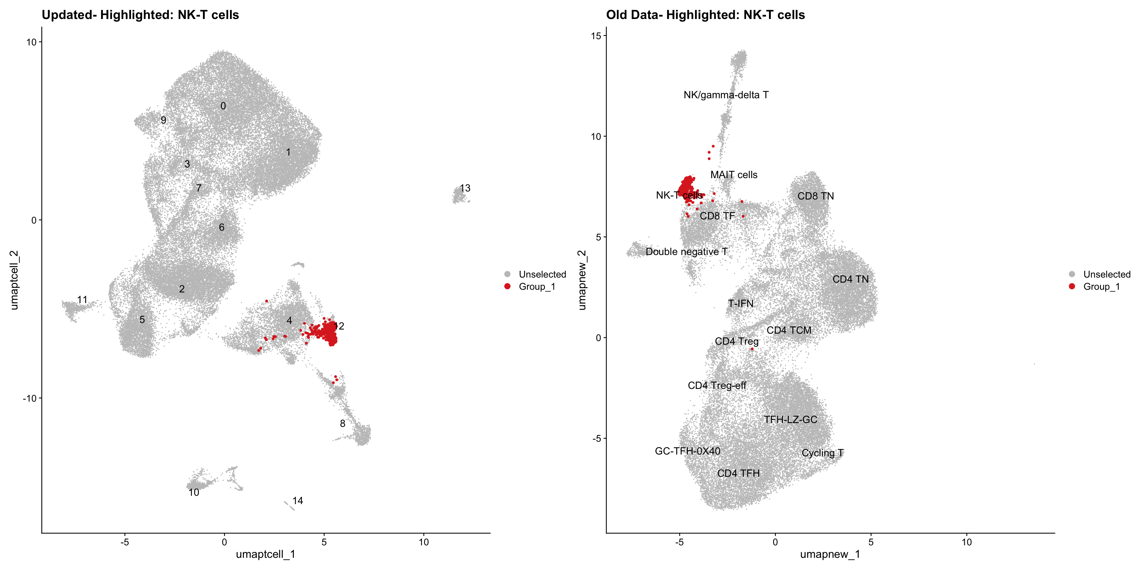
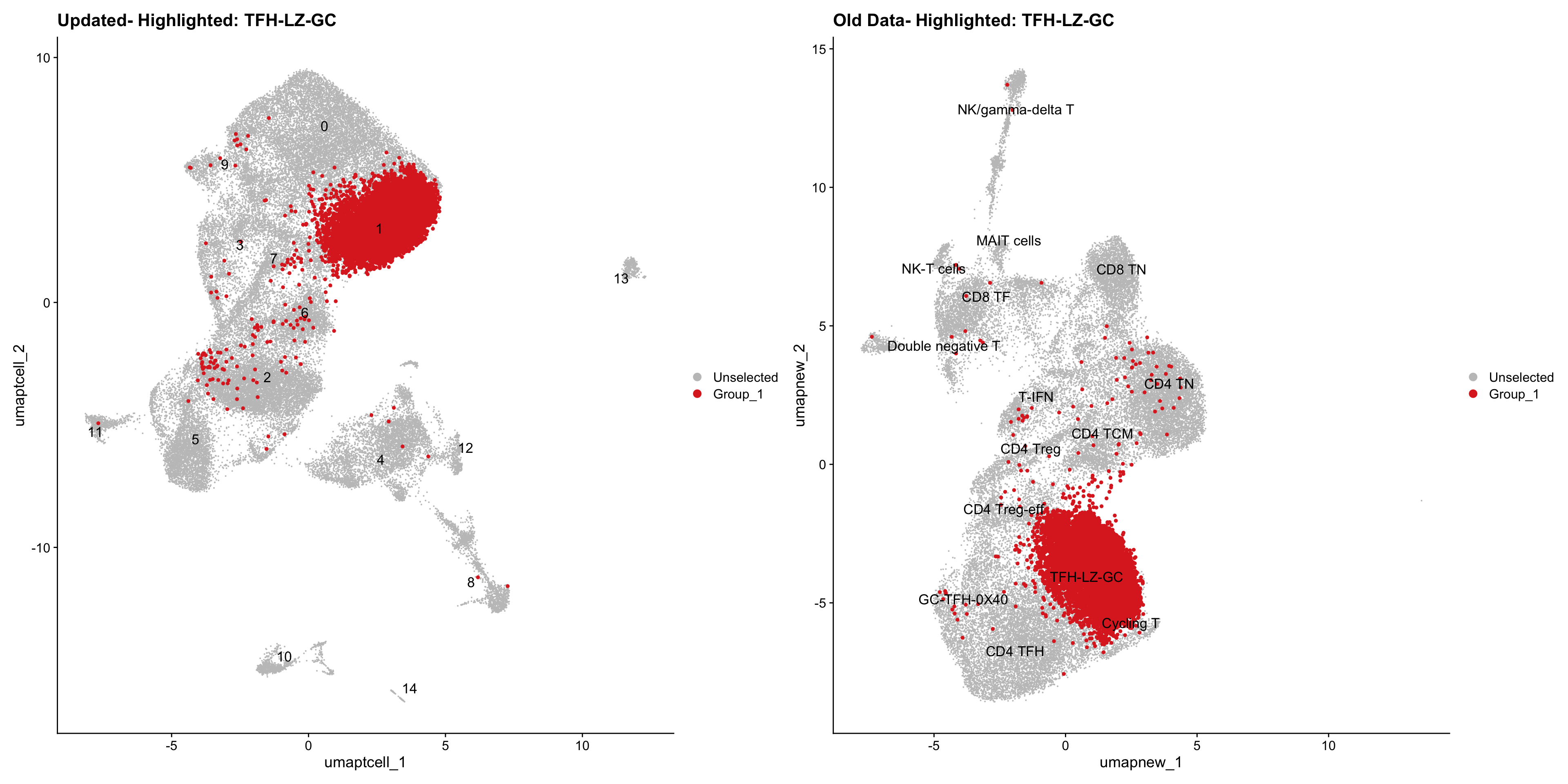
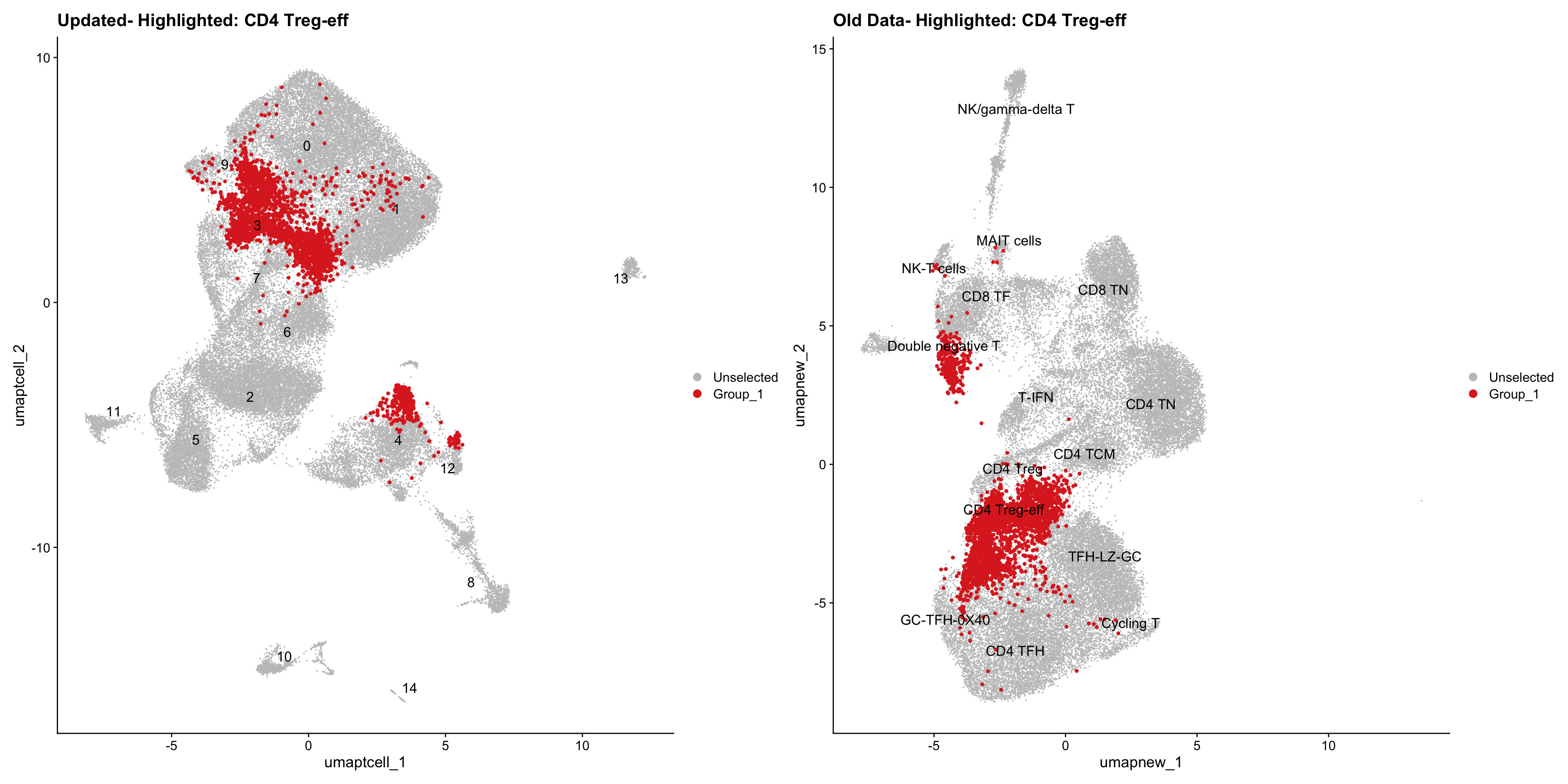
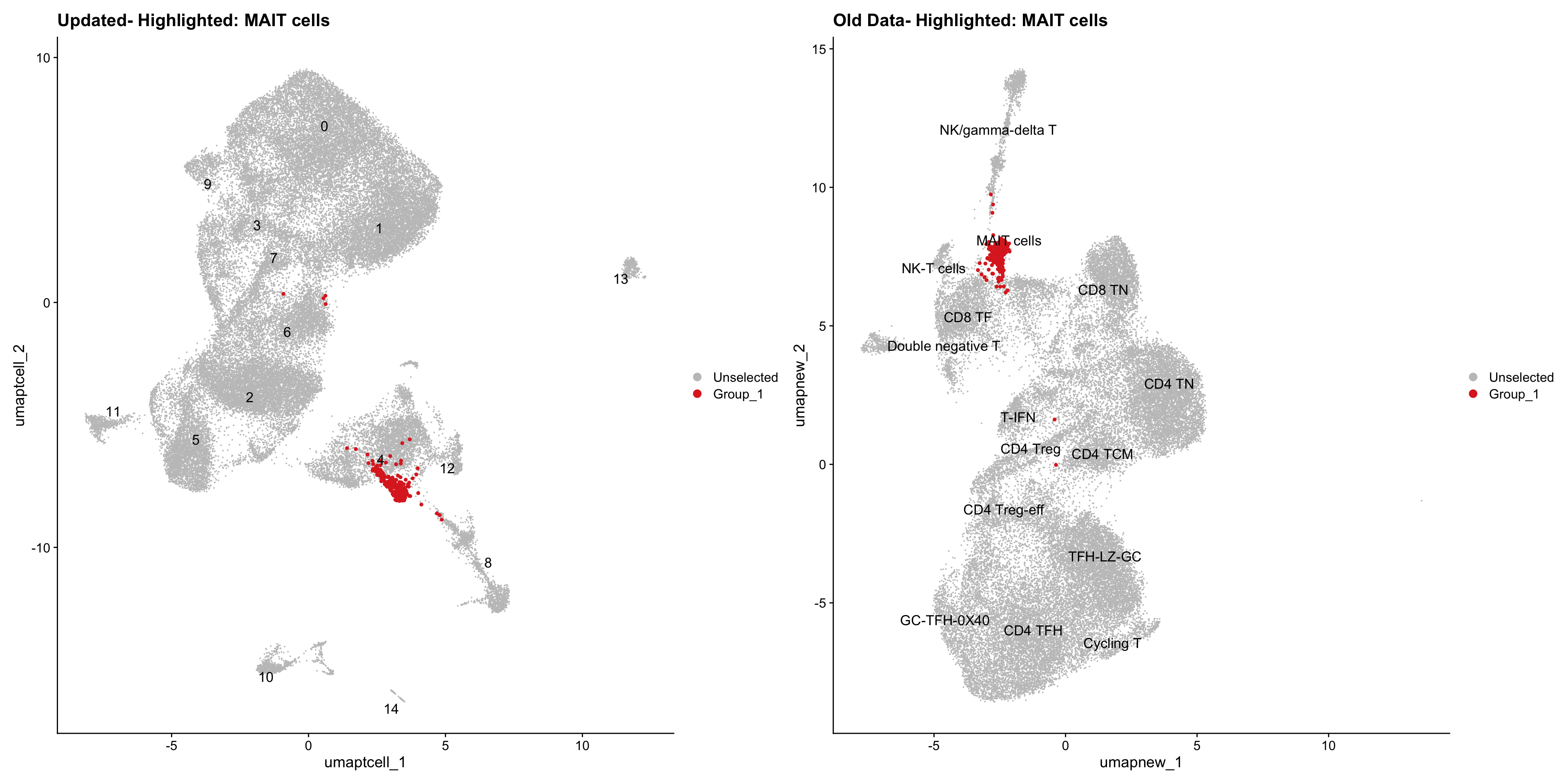
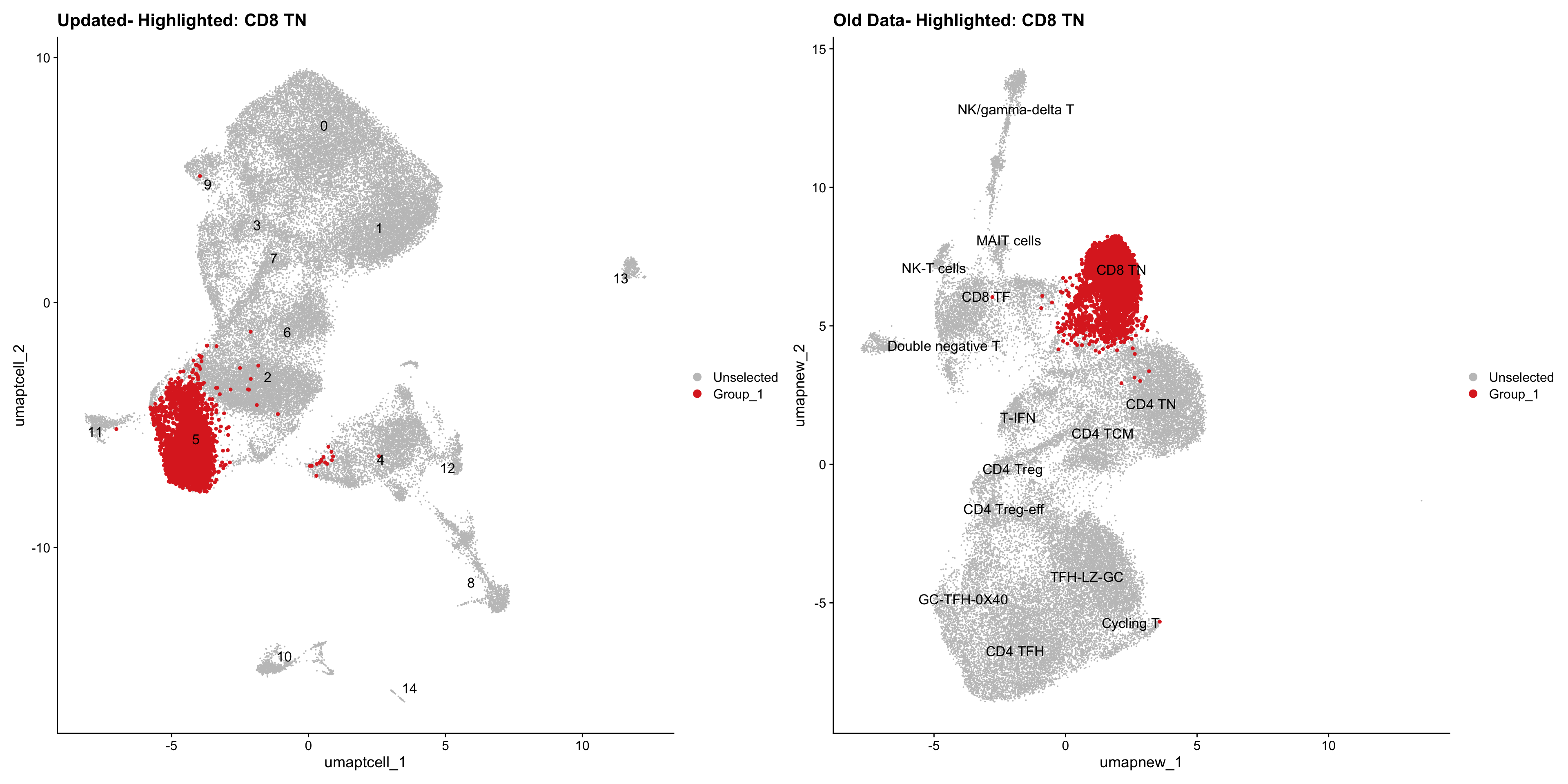
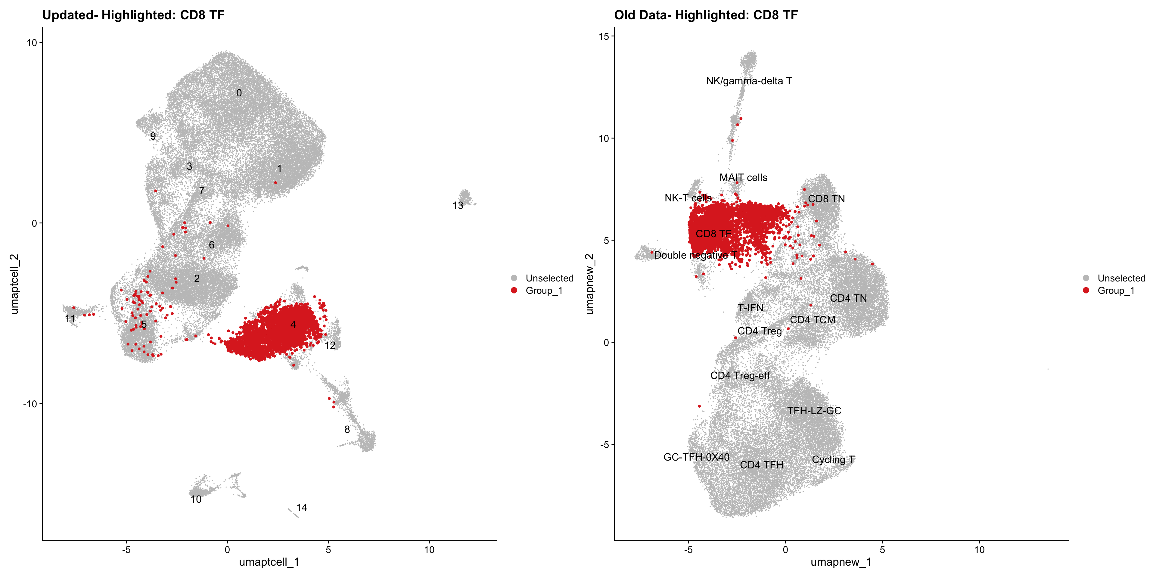
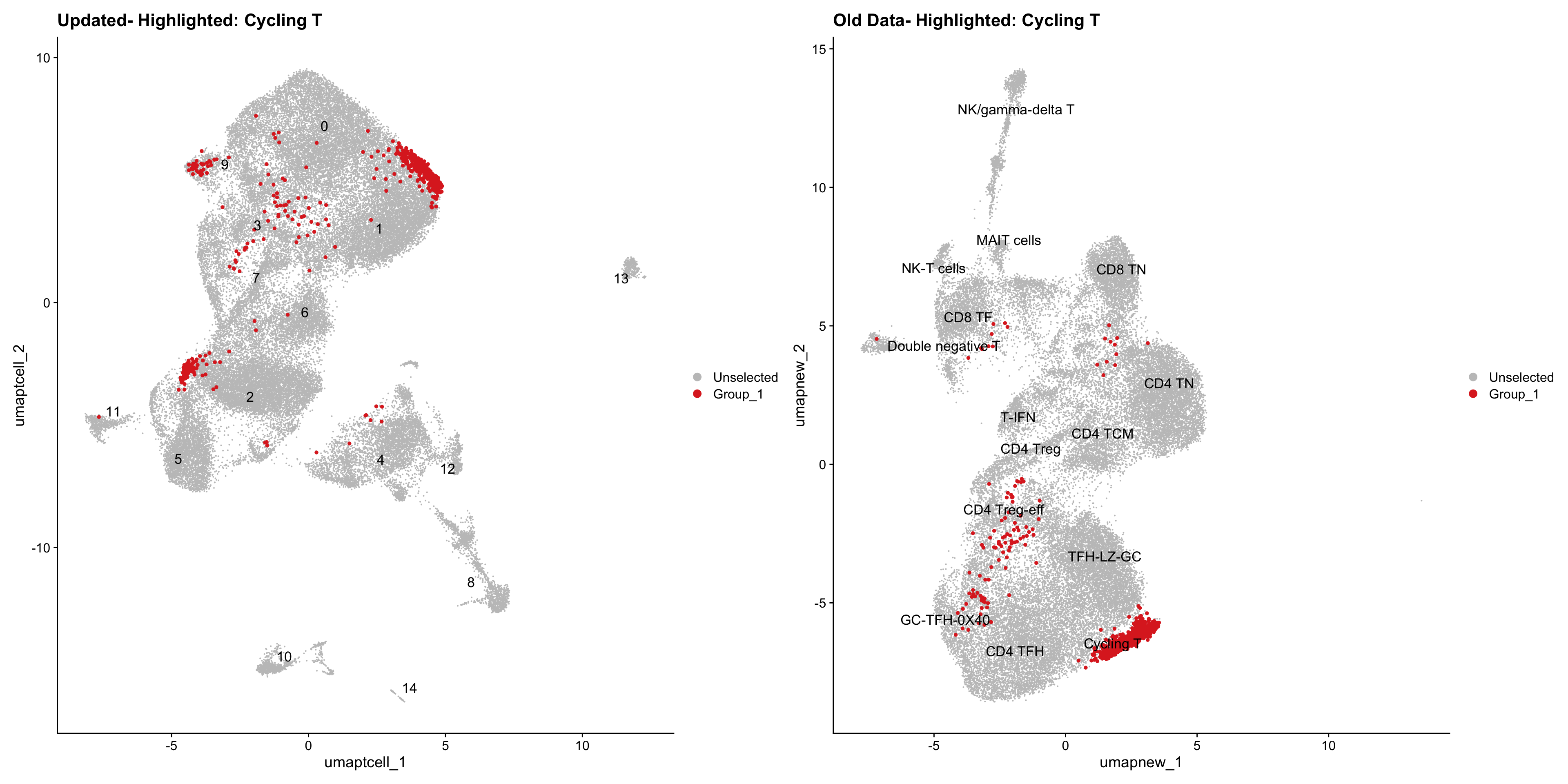
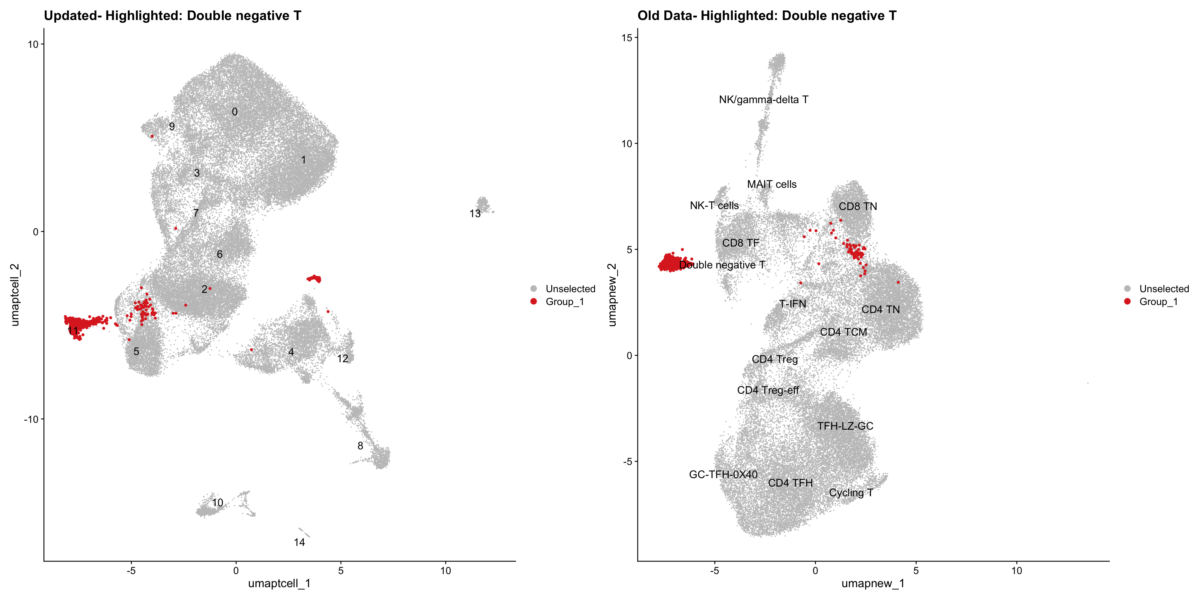
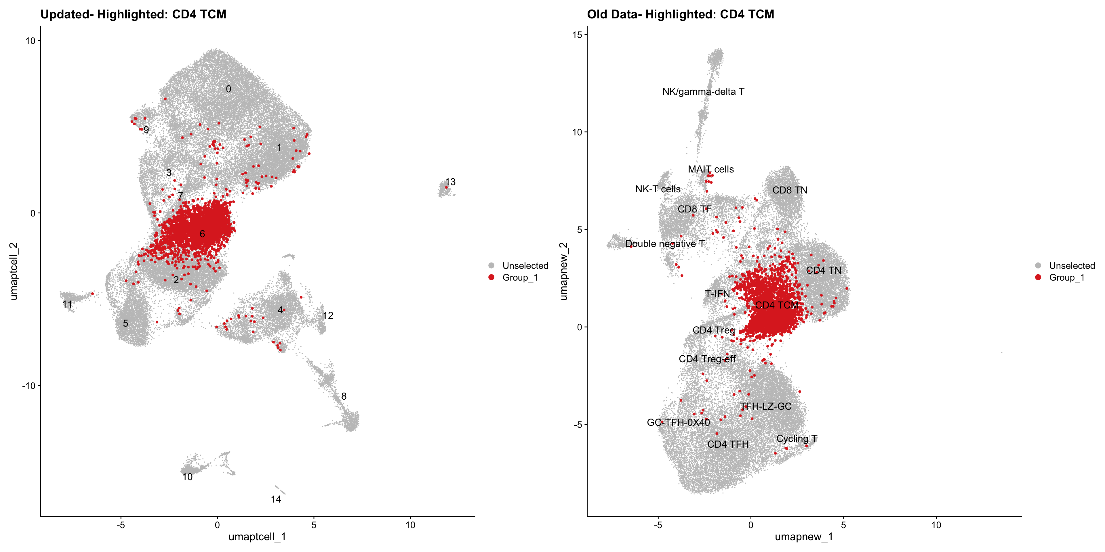
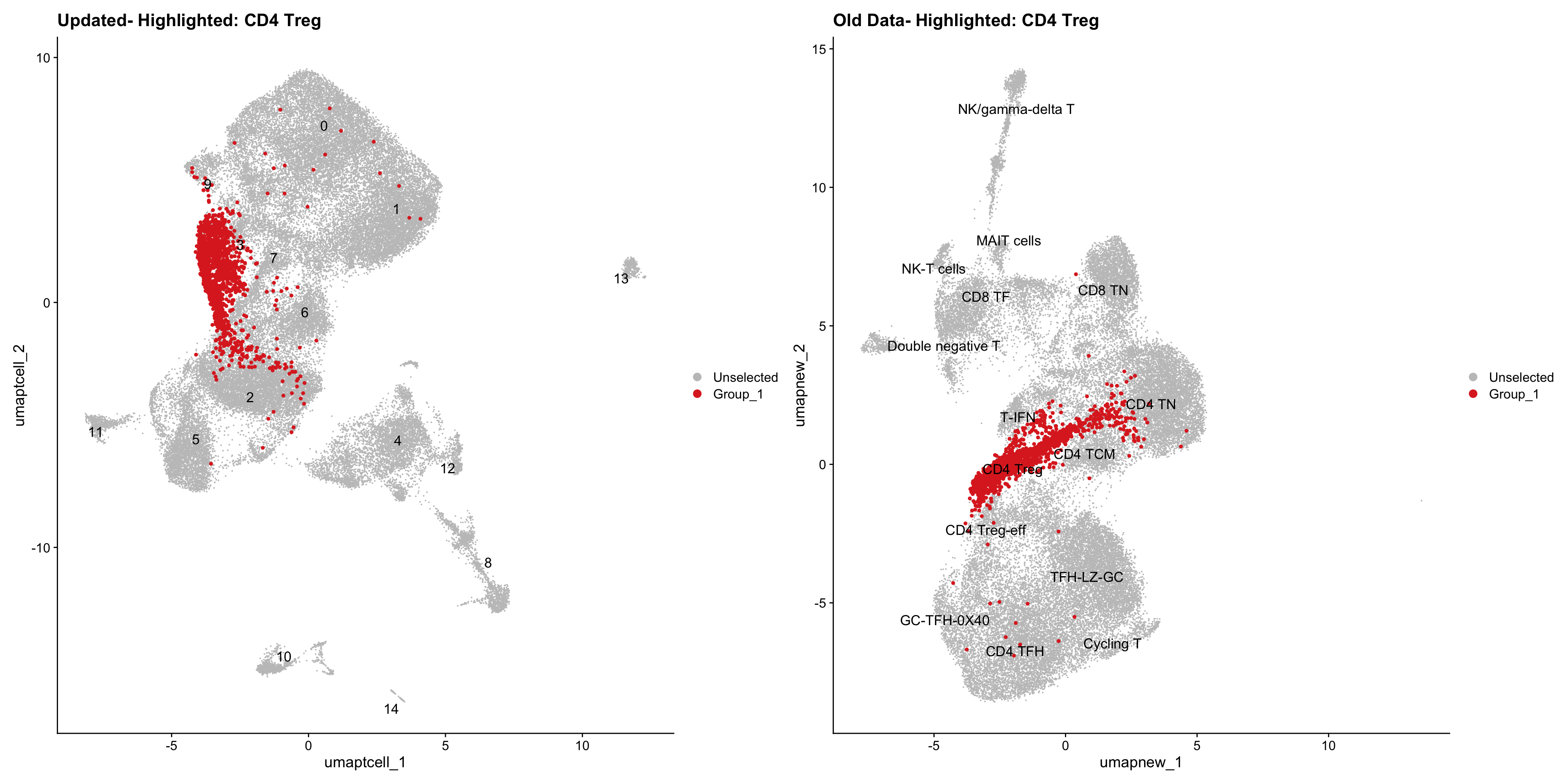
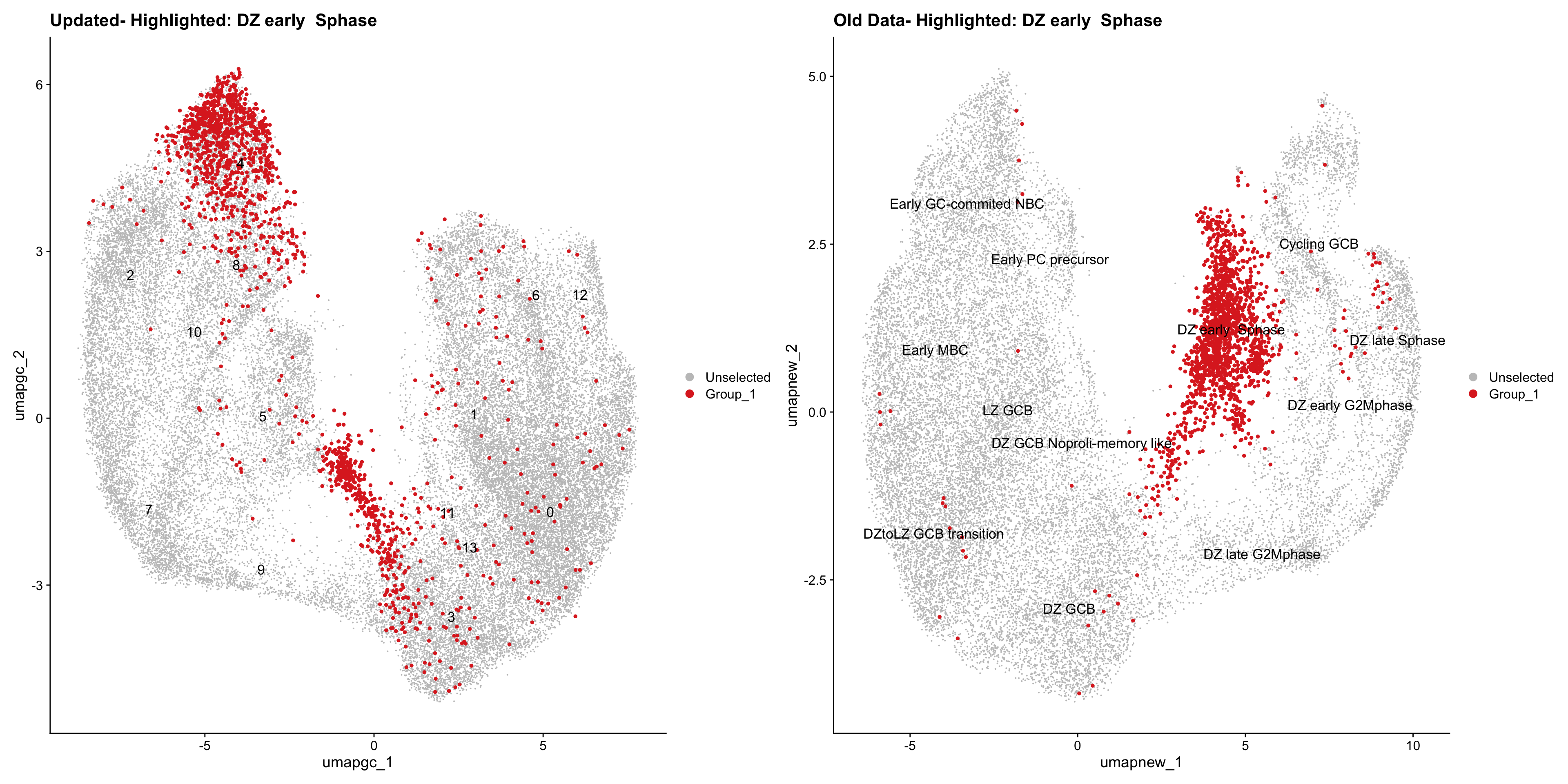
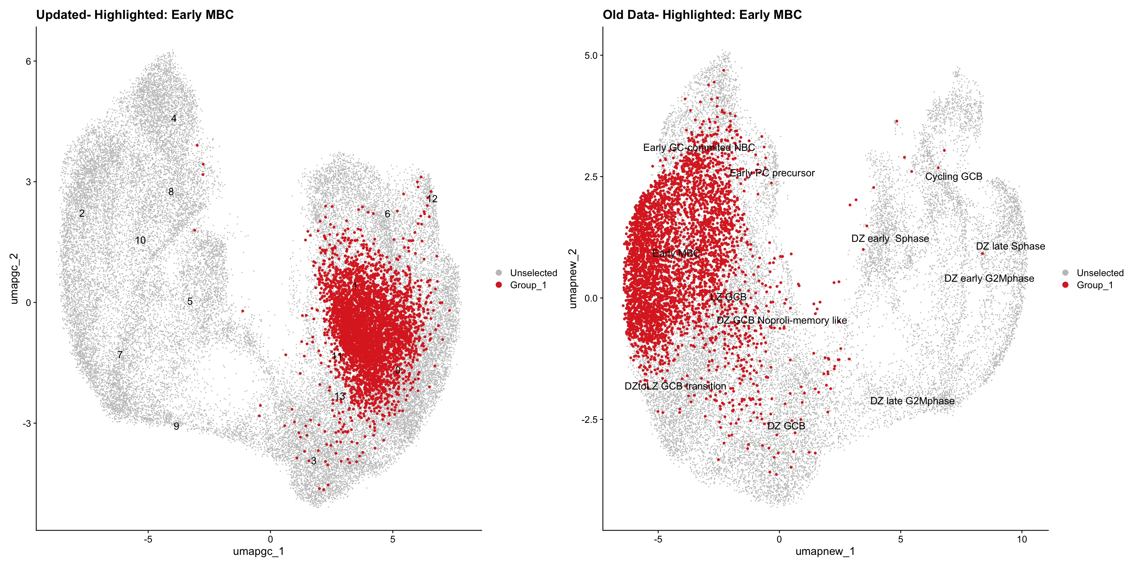
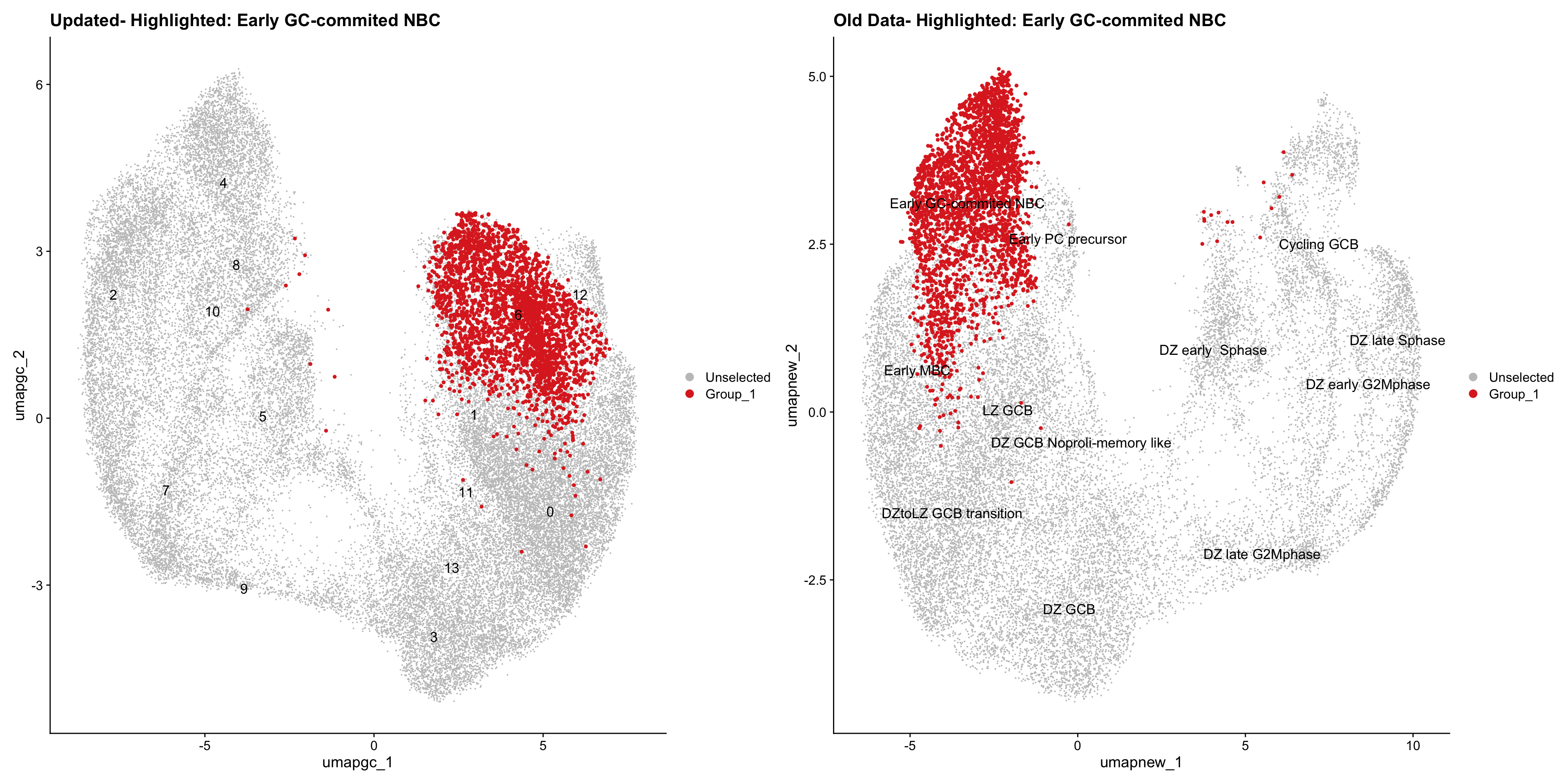
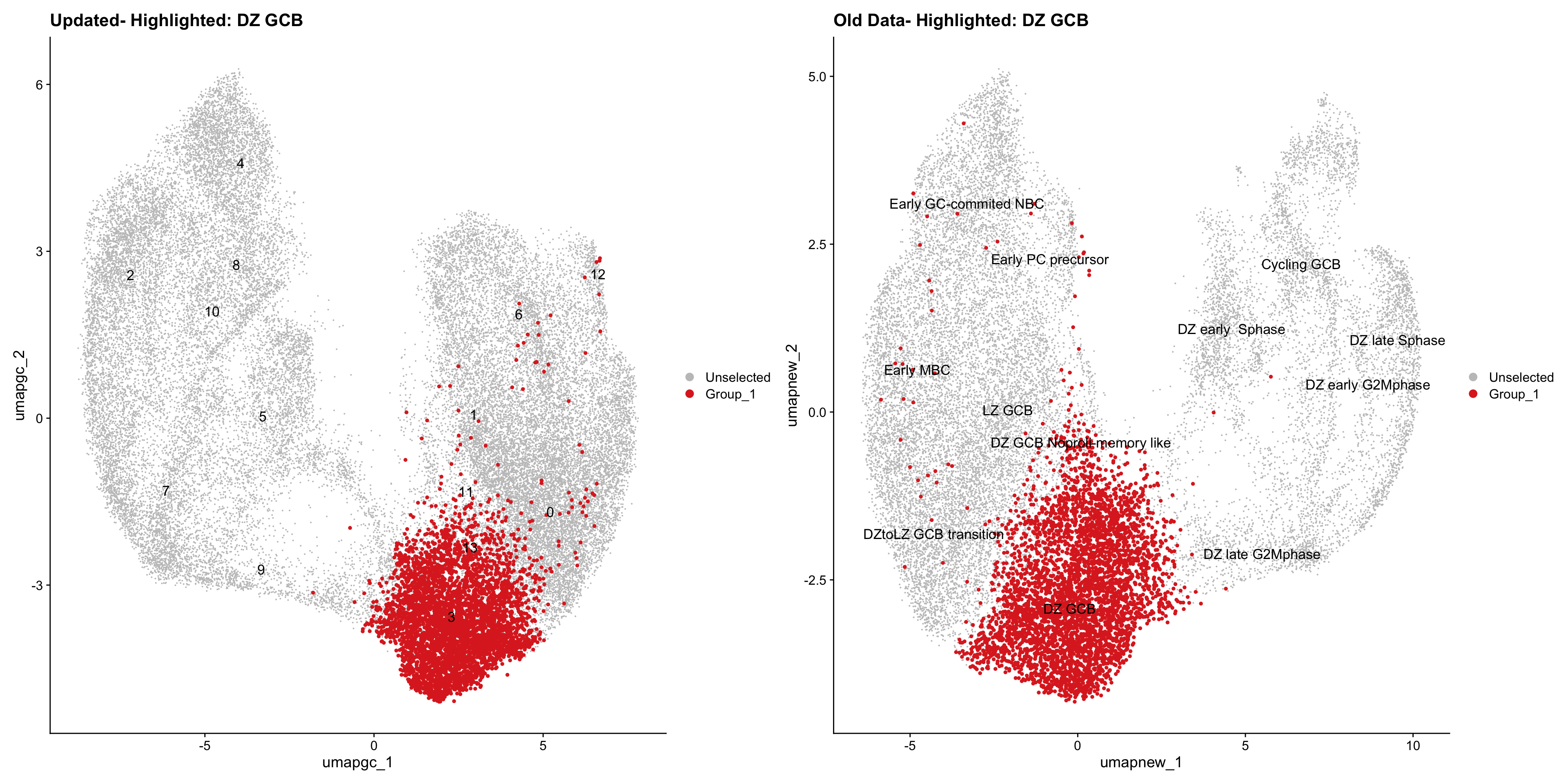
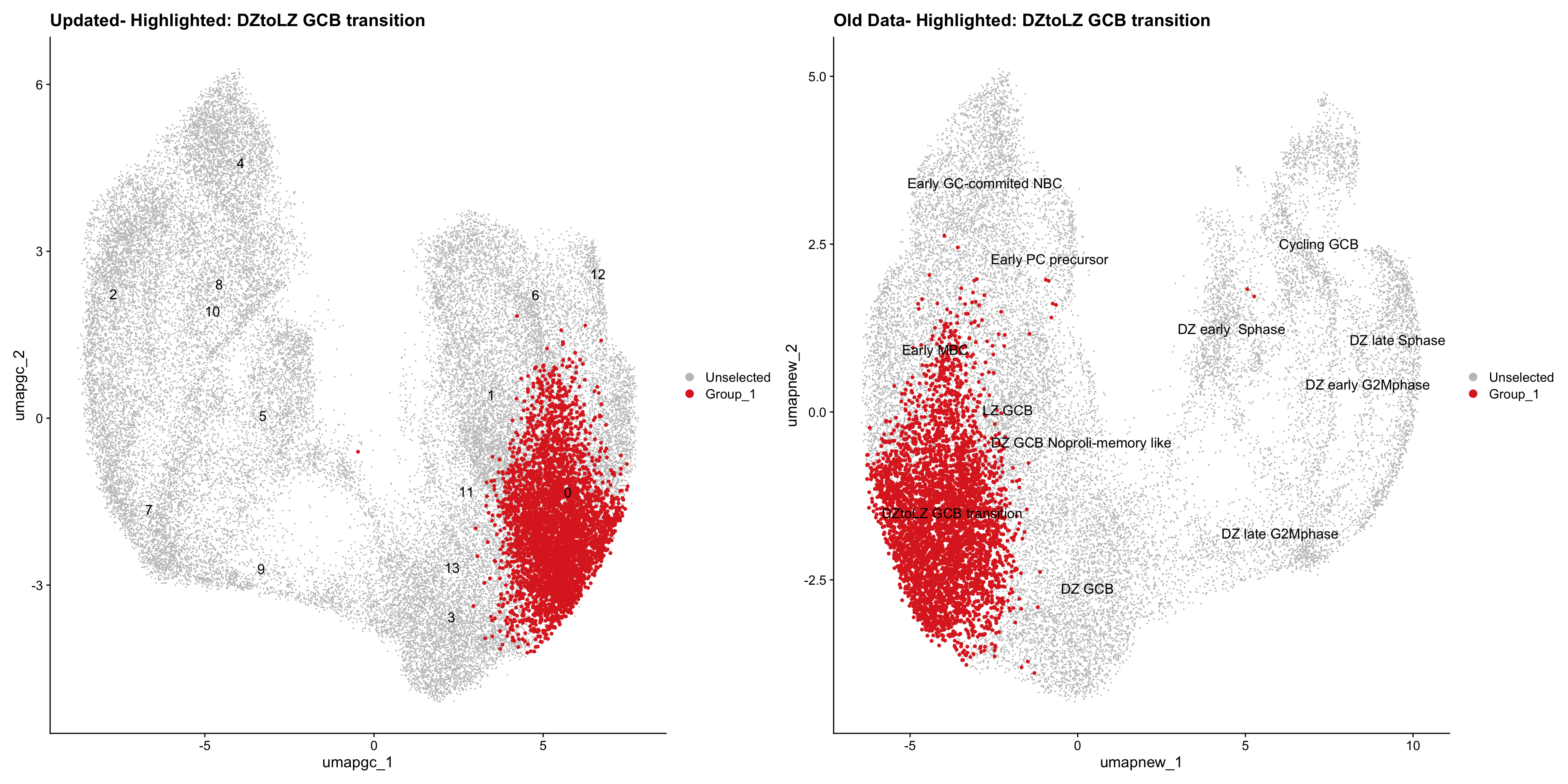
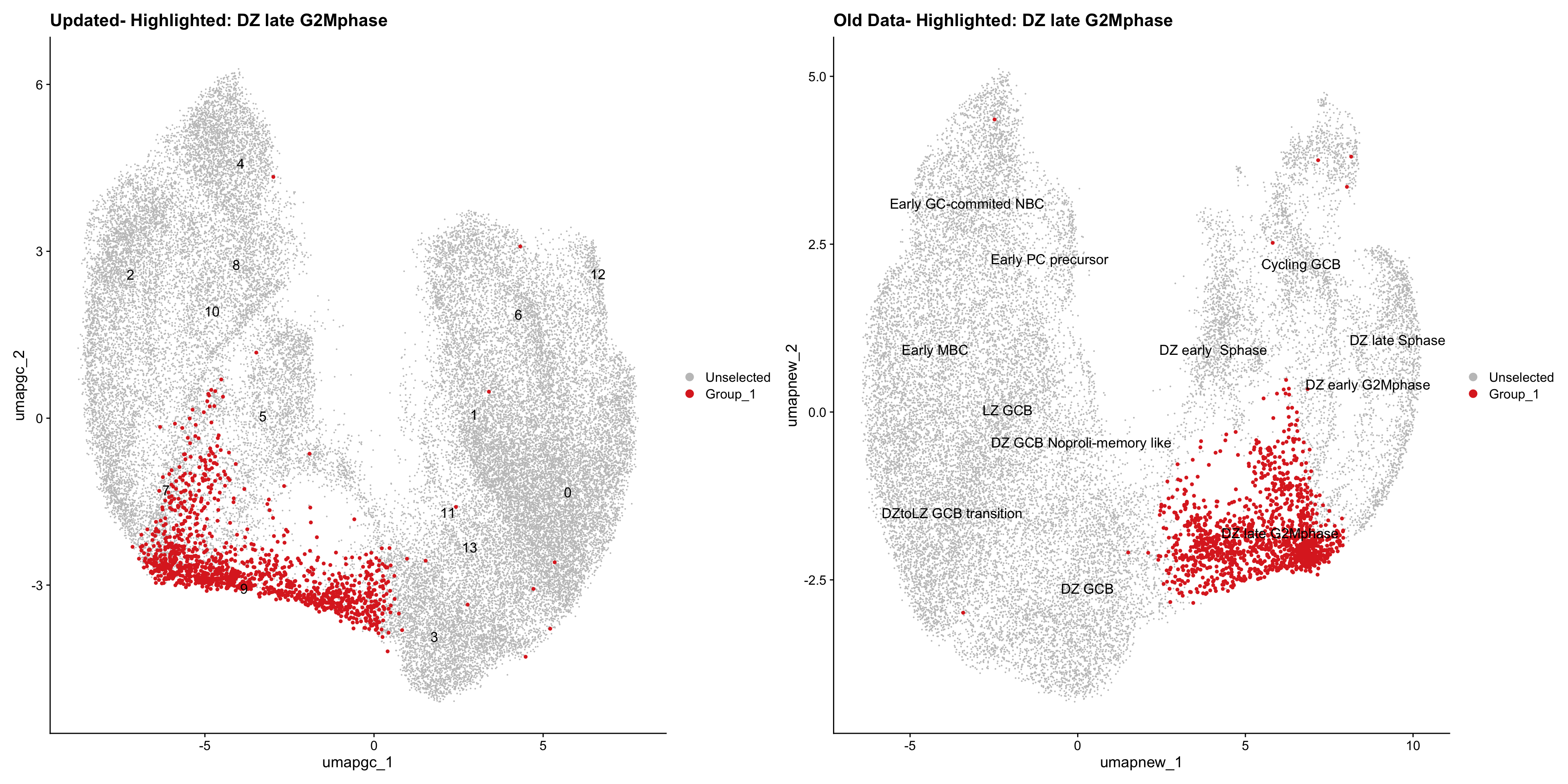
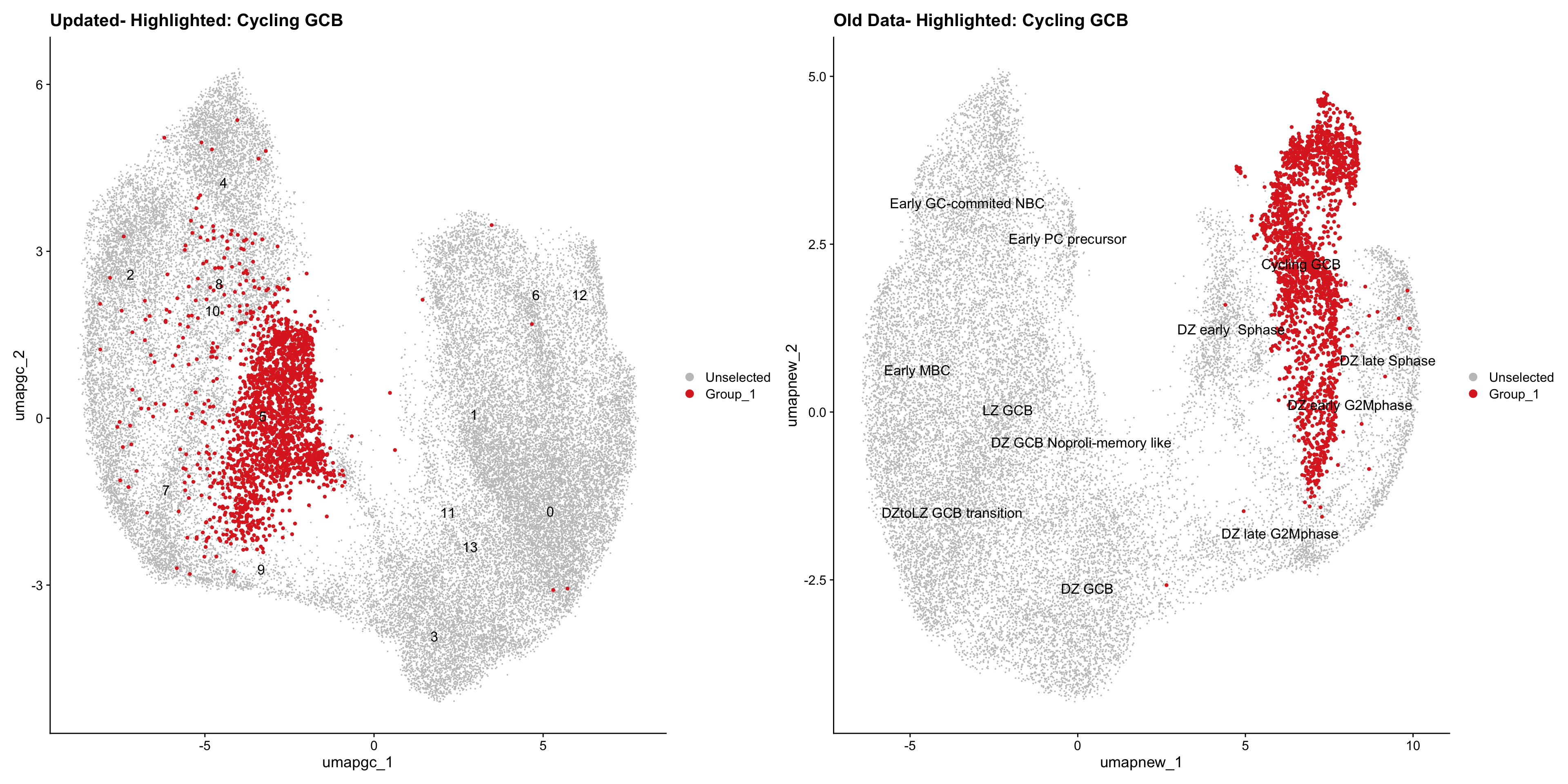
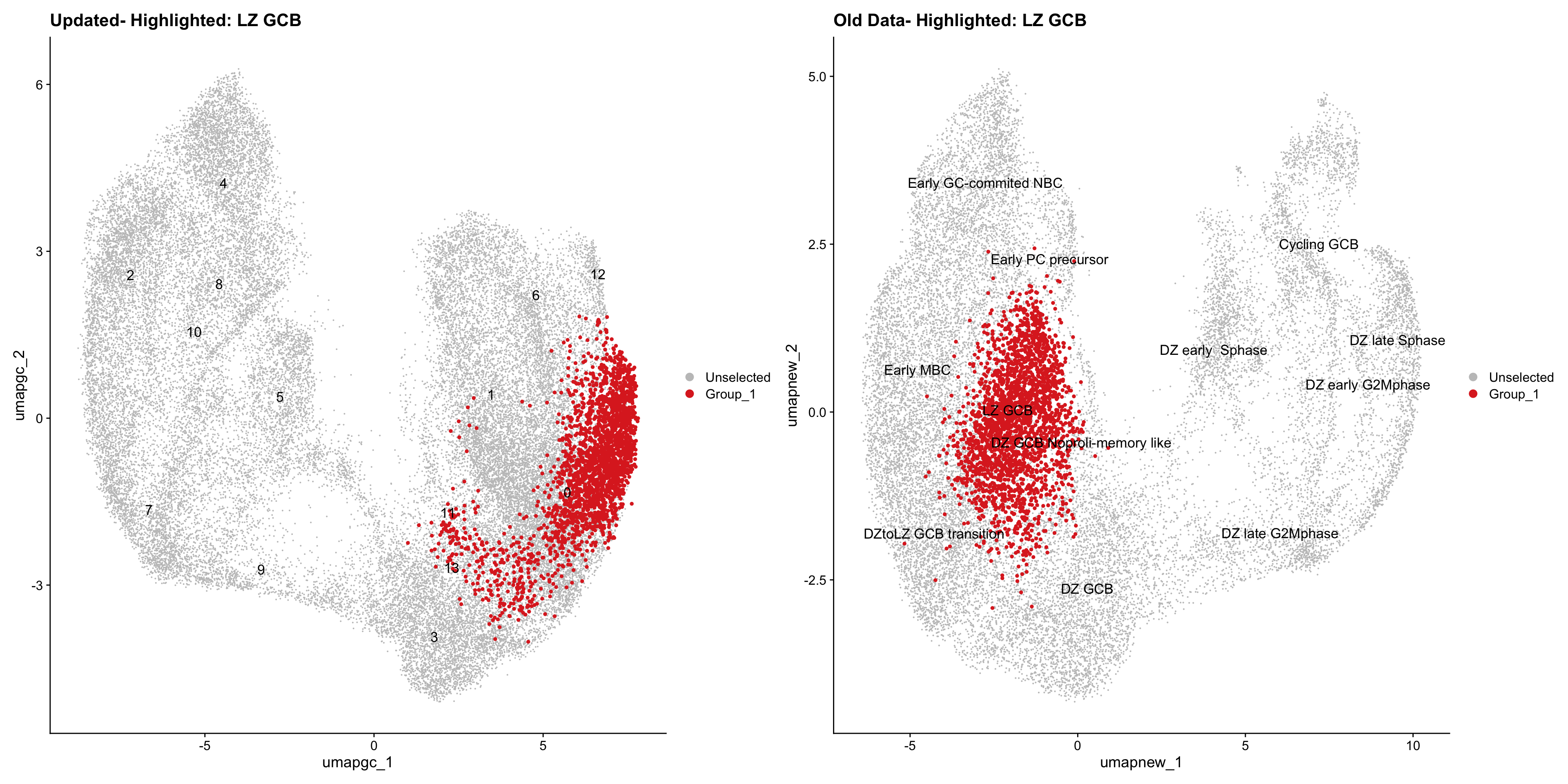
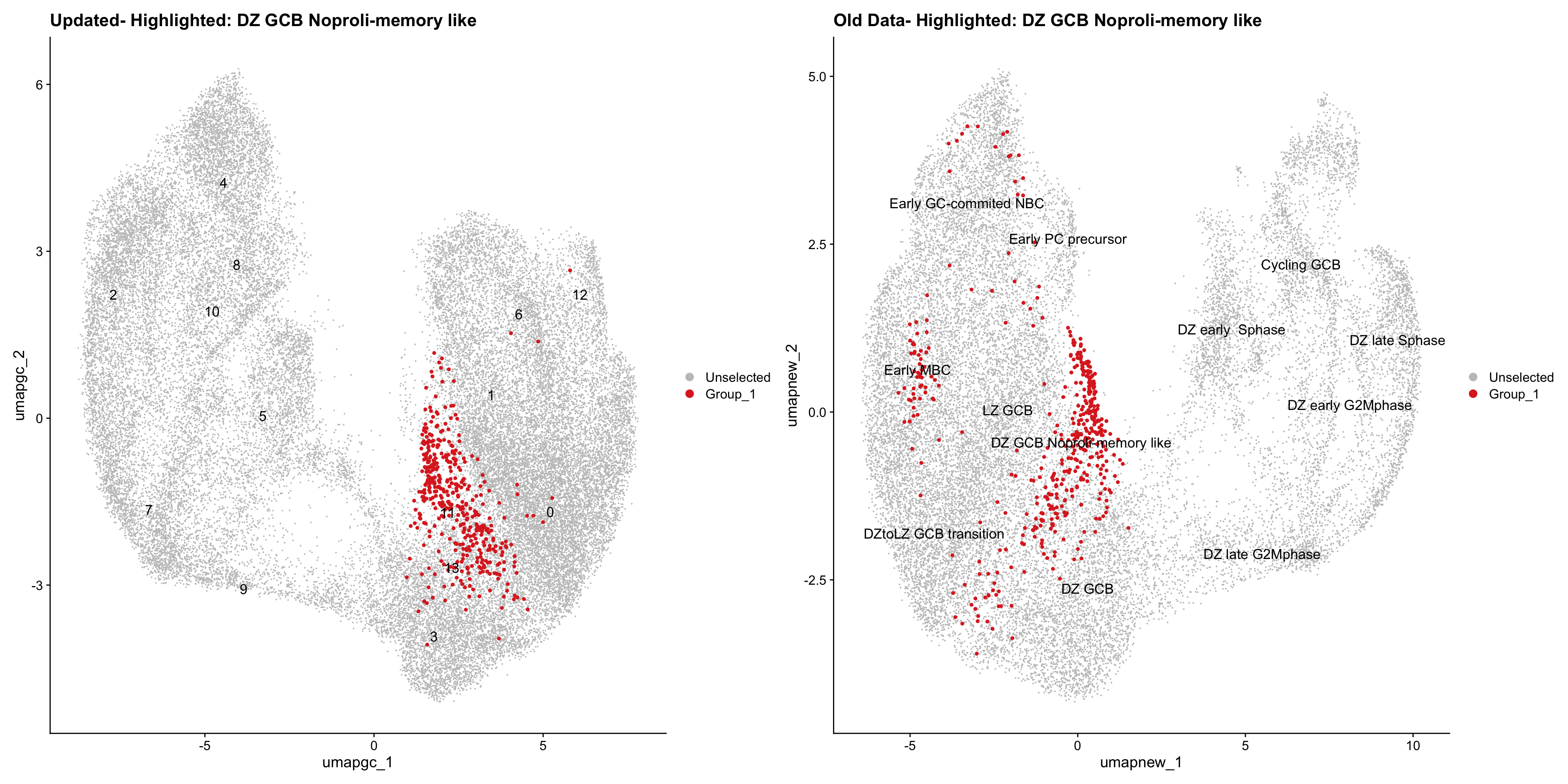
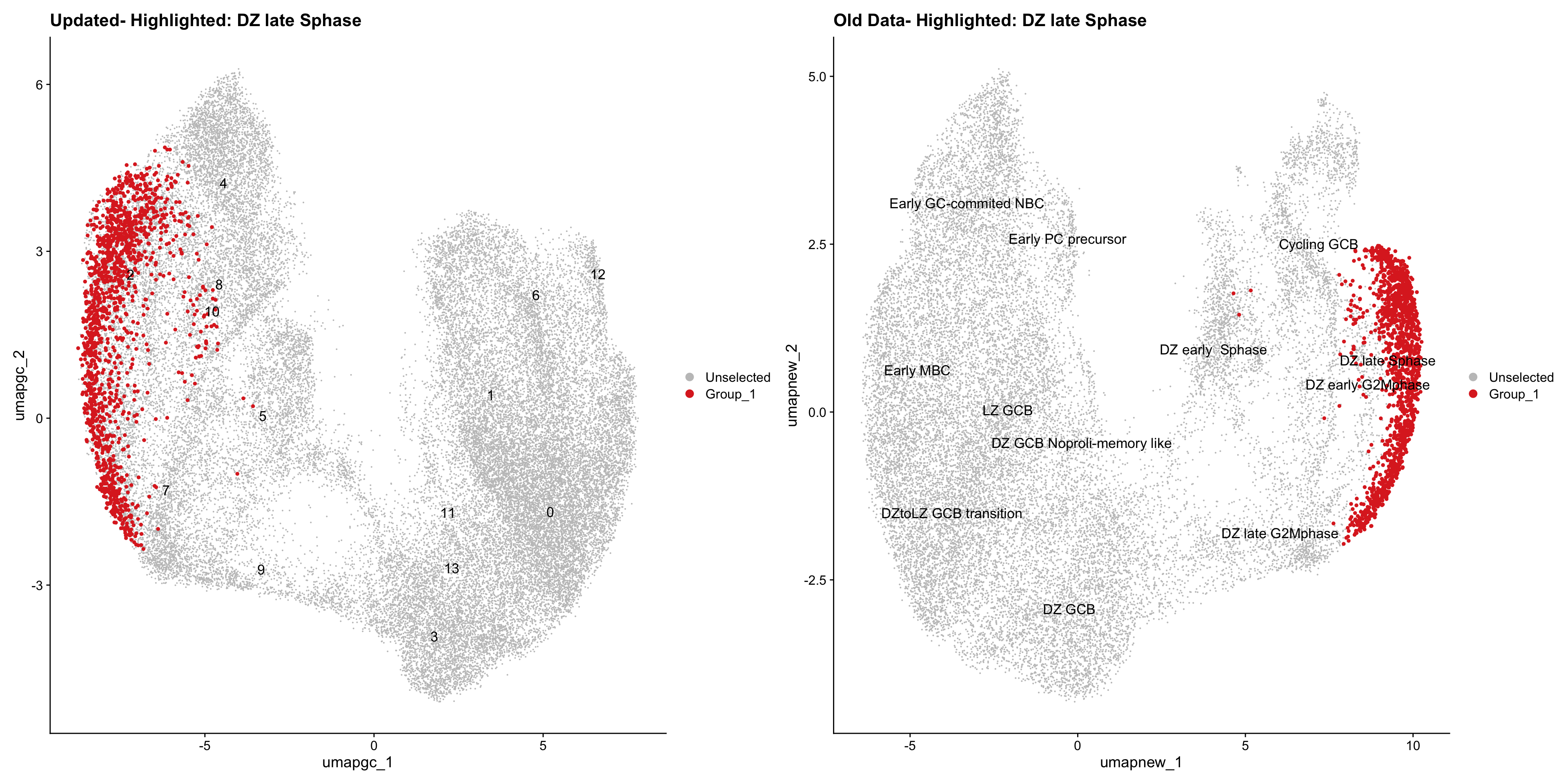
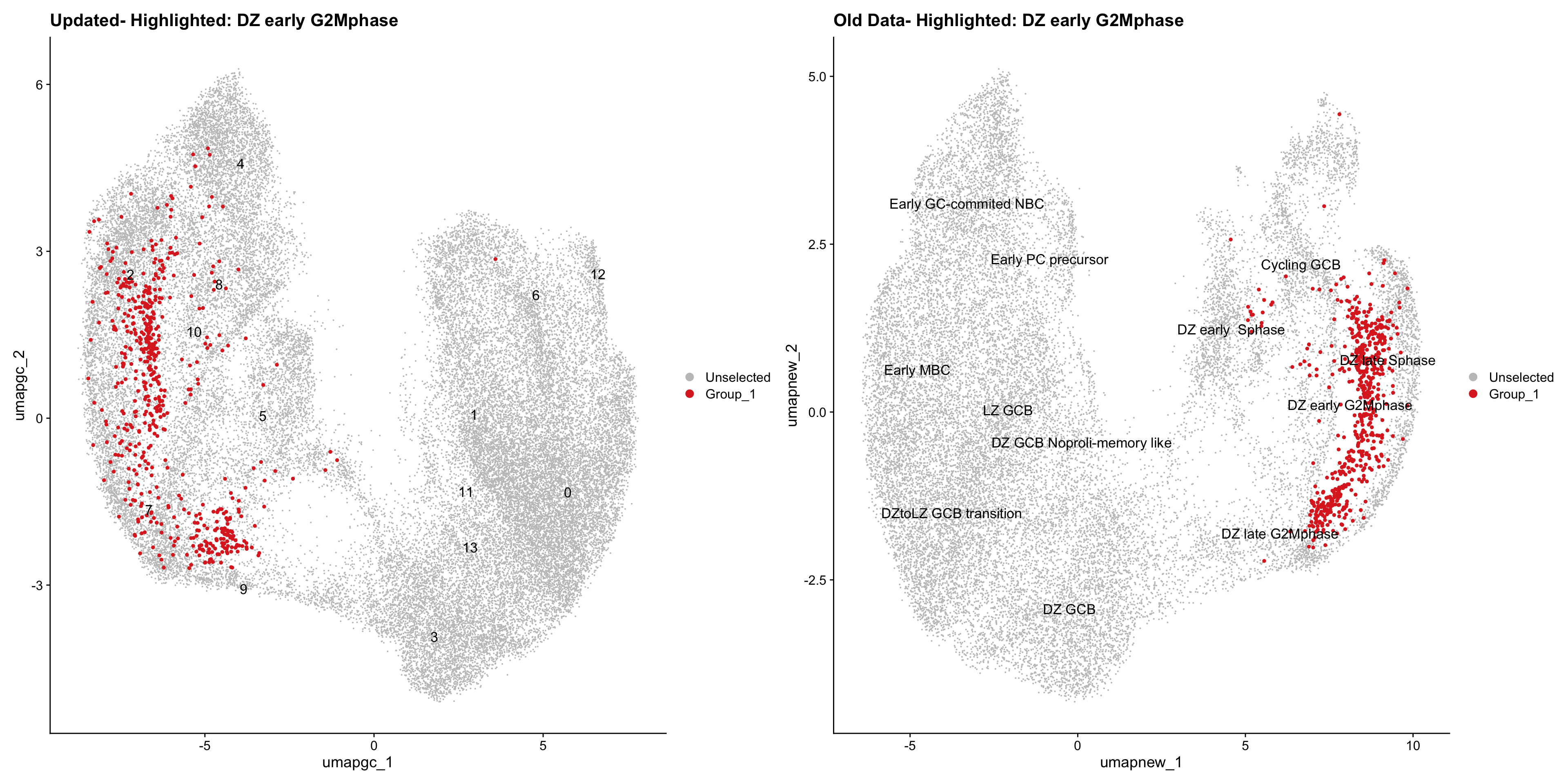
Loading old Subclustering seurat object of T cell population and comparing with the updated clustering.
out2 <- here("output",
"RDS", "AllBatches_Subclustering_SEUs", tissue,
paste0("G000231_Neeland_",tissue,".Tcell_population.subclusters.SEU.rds"))
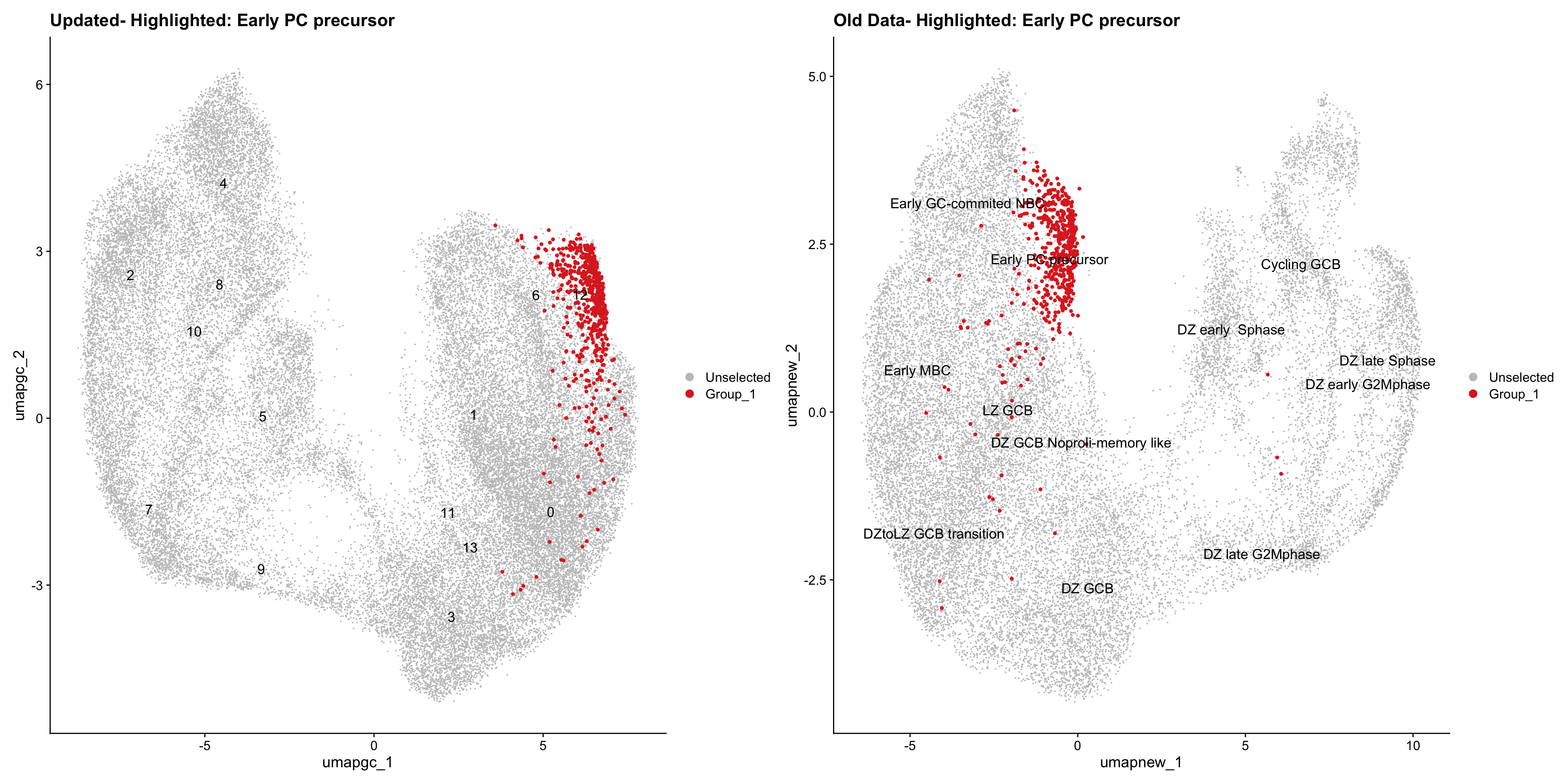
old_obj <- readRDS(out2)cell_types <- unique(old_obj$cell_labels_v2)
for (cell_type in cell_types) {
cl_cells <- WhichCells(old_obj, idents = cell_type)
p <- DimPlot(
paed_sub,
reduction = "umap.tcell",
label = TRUE,
label.size = 4.5,
repel = TRUE,
raster = FALSE,
cells.highlight = cl_cells
) +
ggtitle(paste("Updated- Highlighted:", cell_type))
p1 <- DimPlot(
old_obj,
reduction = "umap.new",
label = T,
label.size = 4.5,
repel = TRUE,
raster = FALSE,
cells.highlight = cl_cells
) +
ggtitle(paste("Old Data- Highlighted:", cell_type))
print(p | p1)
}
| Version | Author | Date |
|---|---|---|
| 54e4ec2 | Gunjan Dixit | 2025-01-08 |
| Version | Author | Date |
|---|---|---|
| 54e4ec2 | Gunjan Dixit | 2025-01-08 |
| Version | Author | Date |
|---|---|---|
| 54e4ec2 | Gunjan Dixit | 2025-01-08 |
| Version | Author | Date |
|---|---|---|
| 54e4ec2 | Gunjan Dixit | 2025-01-08 |
| Version | Author | Date |
|---|---|---|
| 54e4ec2 | Gunjan Dixit | 2025-01-08 |
| Version | Author | Date |
|---|---|---|
| 54e4ec2 | Gunjan Dixit | 2025-01-08 |
| Version | Author | Date |
|---|---|---|
| 54e4ec2 | Gunjan Dixit | 2025-01-08 |
| Version | Author | Date |
|---|---|---|
| 54e4ec2 | Gunjan Dixit | 2025-01-08 |

| Version | Author | Date |
|---|---|---|
| 54e4ec2 | Gunjan Dixit | 2025-01-08 |
| Version | Author | Date |
|---|---|---|
| 54e4ec2 | Gunjan Dixit | 2025-01-08 |
| Version | Author | Date |
|---|---|---|
| 54e4ec2 | Gunjan Dixit | 2025-01-08 |
| Version | Author | Date |
|---|---|---|
| 54e4ec2 | Gunjan Dixit | 2025-01-08 |
| Version | Author | Date |
|---|---|---|
| 54e4ec2 | Gunjan Dixit | 2025-01-08 |
| Version | Author | Date |
|---|---|---|
| 54e4ec2 | Gunjan Dixit | 2025-01-08 |
Save subclustered SEU object (Tcells)
out2 <- here("output",
            "RDS", "AllBatches_Subclustering_SEUs_v2", tissue,
             paste0("G000231_Neeland_",tissue,".Tcell_population.subclusters.SEU.rds"))
#dir.create(out2)
#if (!file.exists(out2)) {
  saveRDS(paed_sub, file = out2)
#}
Updated cell-type labels (T cell clusters)
cell_labels <- readxl::read_excel(here("data/cell_labels_Mel_v4_Dec2024/earlyAIR_Adenoids_all.xlsx"), sheet = "T-reclustering")

new_cluster_names <- cell_labels %>%
  dplyr::select(cluster, annotation) %>%
  deframe()

paed_sub <- RenameIdents(paed_sub, new_cluster_names)
paed_sub@meta.data$cell_labels_v2 <- Idents(paed_sub)

p3 <- DimPlot(paed_sub, reduction = "umap.tcell", raster = FALSE, repel = TRUE, label = TRUE, label.size = 3.5) + ggtitle(paste0(tissue, ": UMAP with Updated T cell population"))

p3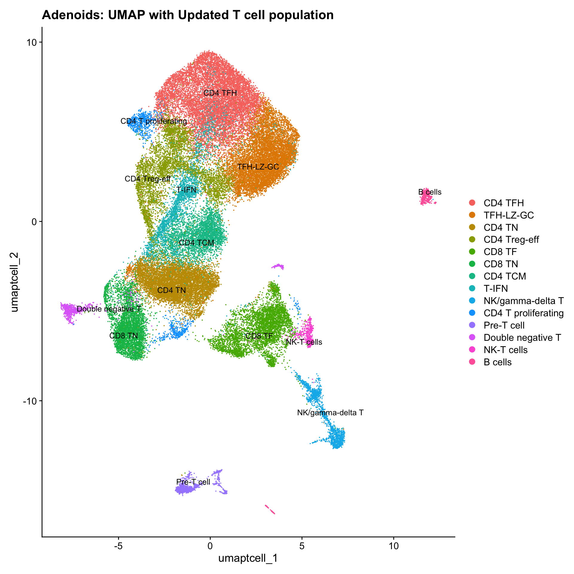
| Version | Author | Date |
|---|---|---|
| 54e4ec2 | Gunjan Dixit | 2025-01-08 |
Save subclustered SEU object
out2 <- here("output",
            "RDS", "AllBatches_Annotated_Subclustering_SEUs_v2", tissue,
             paste0("G000231_Neeland_",tissue,".Tcell_population.subclusters.SEU.rds"))
#dir.create(out2)
if (!file.exists(out2)) {
  saveRDS(paed_sub, file = out2)
}
Reclustering Germinal Center B cells
Reclustering clusters 3,5,8,10
The marker genes for this reclustering can be found here-
Adenoids_GC_population_res.0.6
#sub_clusters <- c(3,5,8,10)

#idx <- which(merged_obj$cluster %in% sub_clusters)
idx <- which(Idents(merged_obj) %in% "Germinal centre B cells for reclustering")
paed_gc <- merged_obj[,idx]
paed_gc
An object of class Seurat
17456 features across 42615 samples within 1 assay
Active assay: RNA (17456 features, 2000 variable features)
3 layers present: data, counts, scale.data
4 dimensional reductions calculated: pca, umap.unintegrated, harmony, umap.harmony# Visualize the clustering results
DimPlot(paed_gc, reduction = "umap.harmony", group.by = "cluster", label = TRUE, label.size = 2.5, repel = TRUE, raster = FALSE )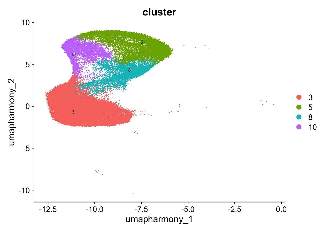
| Version | Author | Date |
|---|---|---|
| 54e4ec2 | Gunjan Dixit | 2025-01-08 |
paed_gc <- paed_gc %>%
  NormalizeData() %>%
  FindVariableFeatures() %>%
  ScaleData() %>%
  RunPCA()

paed_gc <- RunUMAP(paed_gc, dims = 1:30, reduction = "pca", reduction.name = "umap.gc")
meta_data_columns <- colnames(paed_gc@meta.data)
columns_to_remove <- grep("^RNA_snn_res", meta_data_columns, value = TRUE)
paed_gc@meta.data <- paed_gc@meta.data[, !(colnames(paed_gc@meta.data) %in% columns_to_remove)]resolutions <- seq(0.1, 1, by = 0.1)
paed_gc <- FindNeighbors(paed_gc, dims = 1:30, reduction = "pca")
paed_gc <- FindClusters(paed_gc, resolution = resolutions )Modularity Optimizer version 1.3.0 by Ludo Waltman and Nees Jan van Eck
Number of nodes: 42615
Number of edges: 1259614
Running Louvain algorithm...
Maximum modularity in 10 random starts: 0.9426
Number of communities: 2
Elapsed time: 8 seconds
Modularity Optimizer version 1.3.0 by Ludo Waltman and Nees Jan van Eck
Number of nodes: 42615
Number of edges: 1259614
Running Louvain algorithm...
Maximum modularity in 10 random starts: 0.9142
Number of communities: 5
Elapsed time: 7 seconds
Modularity Optimizer version 1.3.0 by Ludo Waltman and Nees Jan van Eck
Number of nodes: 42615
Number of edges: 1259614
Running Louvain algorithm...
Maximum modularity in 10 random starts: 0.8959
Number of communities: 8
Elapsed time: 7 seconds
Modularity Optimizer version 1.3.0 by Ludo Waltman and Nees Jan van Eck
Number of nodes: 42615
Number of edges: 1259614
Running Louvain algorithm...
Maximum modularity in 10 random starts: 0.8813
Number of communities: 10
Elapsed time: 7 seconds
Modularity Optimizer version 1.3.0 by Ludo Waltman and Nees Jan van Eck
Number of nodes: 42615
Number of edges: 1259614
Running Louvain algorithm...
Maximum modularity in 10 random starts: 0.8681
Number of communities: 11
Elapsed time: 7 seconds
Modularity Optimizer version 1.3.0 by Ludo Waltman and Nees Jan van Eck
Number of nodes: 42615
Number of edges: 1259614
Running Louvain algorithm...
Maximum modularity in 10 random starts: 0.8559
Number of communities: 14
Elapsed time: 6 seconds
Modularity Optimizer version 1.3.0 by Ludo Waltman and Nees Jan van Eck
Number of nodes: 42615
Number of edges: 1259614
Running Louvain algorithm...
Maximum modularity in 10 random starts: 0.8472
Number of communities: 15
Elapsed time: 7 seconds
Modularity Optimizer version 1.3.0 by Ludo Waltman and Nees Jan van Eck
Number of nodes: 42615
Number of edges: 1259614
Running Louvain algorithm...
Maximum modularity in 10 random starts: 0.8389
Number of communities: 16
Elapsed time: 6 seconds
Modularity Optimizer version 1.3.0 by Ludo Waltman and Nees Jan van Eck
Number of nodes: 42615
Number of edges: 1259614
Running Louvain algorithm...
Maximum modularity in 10 random starts: 0.8312
Number of communities: 17
Elapsed time: 7 seconds
Modularity Optimizer version 1.3.0 by Ludo Waltman and Nees Jan van Eck
Number of nodes: 42615
Number of edges: 1259614
Running Louvain algorithm...
Maximum modularity in 10 random starts: 0.8239
Number of communities: 19
Elapsed time: 6 secondsclustree(paed_gc, prefix = "RNA_snn_res.")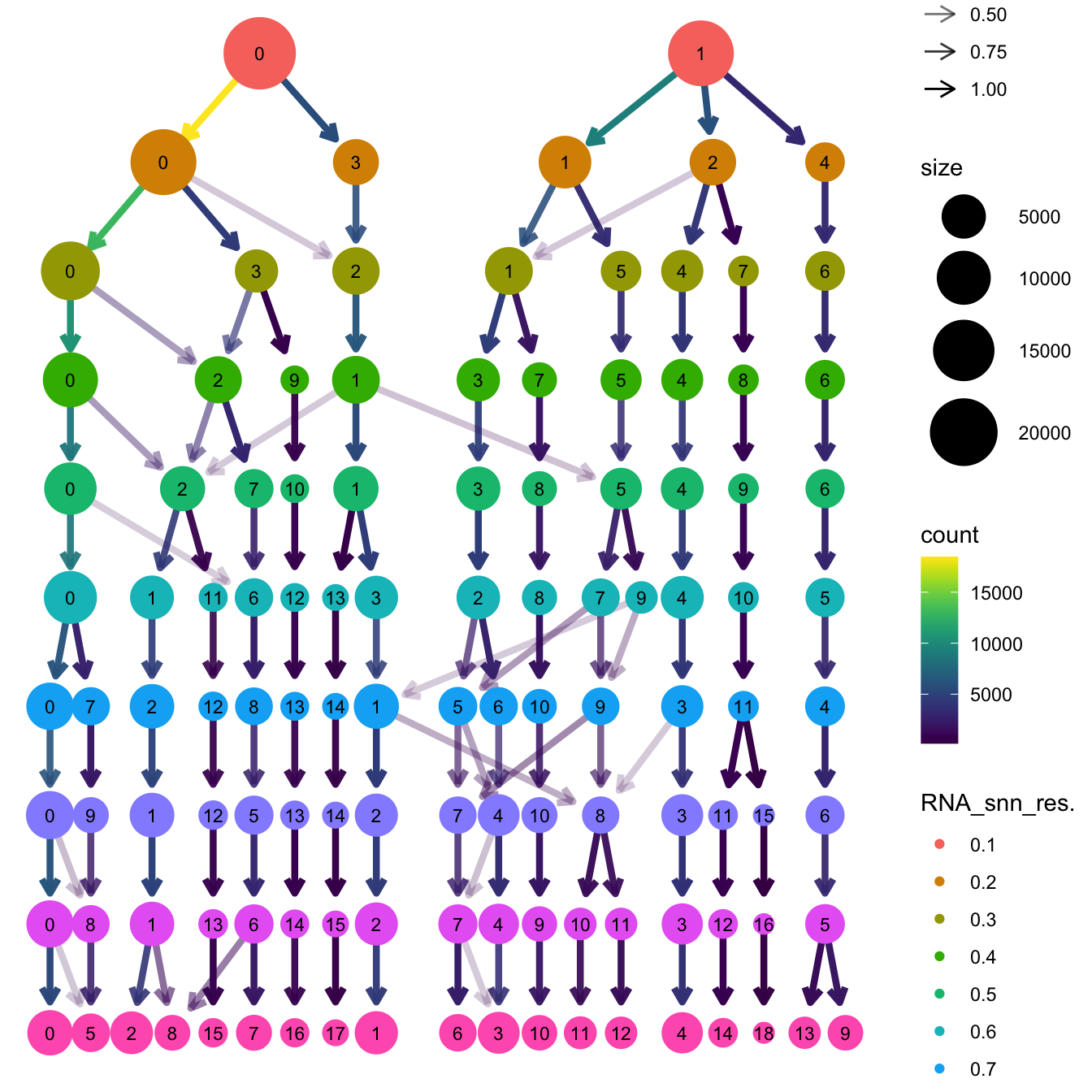
| Version | Author | Date |
|---|---|---|
| 54e4ec2 | Gunjan Dixit | 2025-01-08 |
# Visualize the clustering results
DimPlot(paed_gc, group.by = "RNA_snn_res.0.6", reduction = "umap.gc", label = TRUE, label.size = 2.5, repel = TRUE, raster = FALSE )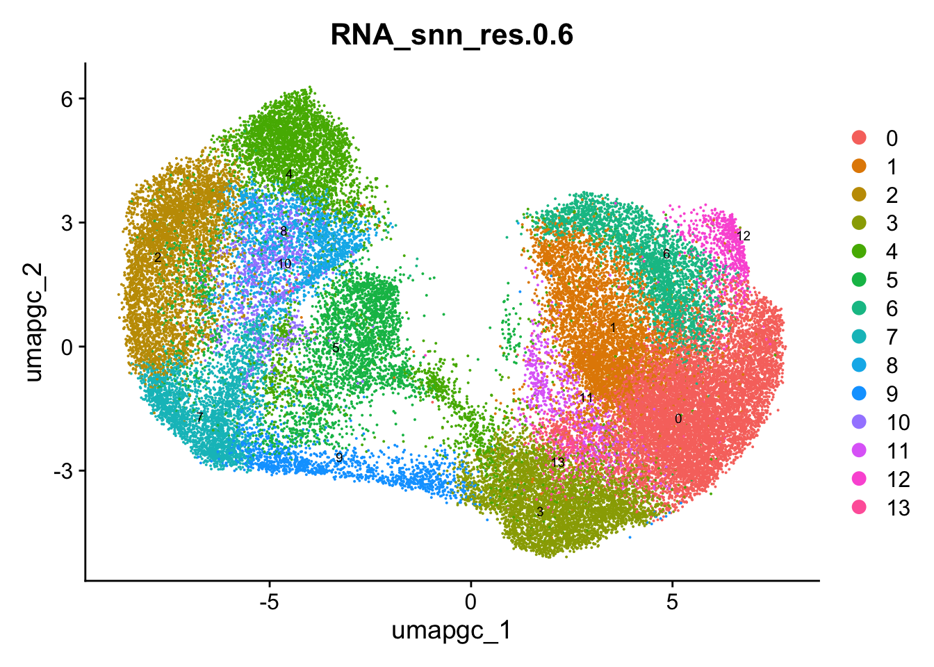
opt_res <- "RNA_snn_res.0.6"
n <- nlevels(paed_gc$RNA_snn_res.0.6)
paed_gc$RNA_snn_res.0.6 <- factor(paed_gc$RNA_snn_res.0.6, levels = seq(0,n-1))
paed_gc$seurat_clusters <- NULL
paed_gc$cluster <- paed_gc$RNA_snn_res.0.6
Idents(paed_gc) <- paed_gc$cluster
paed_gc.markers <- FindAllMarkers(paed_gc, only.pos = TRUE, min.pct = 0.25, logfc.threshold = 0.25)Calculating cluster 0Calculating cluster 1Calculating cluster 2Calculating cluster 3Calculating cluster 4Calculating cluster 5Calculating cluster 6Calculating cluster 7Calculating cluster 8Calculating cluster 9Calculating cluster 10Calculating cluster 11Calculating cluster 12Calculating cluster 13paed_gc.markers %>%
group_by(cluster) %>% unique() %>%
top_n(n = 5, wt = avg_log2FC) -> top5
paed_gc.markers %>%
group_by(cluster) %>%
slice_head(n=1) %>%
pull(gene) -> best.wilcox.gene.per.cluster
best.wilcox.gene.per.cluster [1] "FCRL3" "FCRL5" "HIST1H2BB" "AICDA" "MCM4" "TYMS"
[7] "DUSP2" "KIF20A" "SLC43A3" "CDC20" "TNFRSF13B" "SLA"
[13] "PRDM1" "CHAC1" Feature plot shows the expression of top marker genes per cluster.
FeaturePlot(paed_gc,features=best.wilcox.gene.per.cluster, reduction = 'umap.gc', raster = FALSE, ncol = 2, label = TRUE)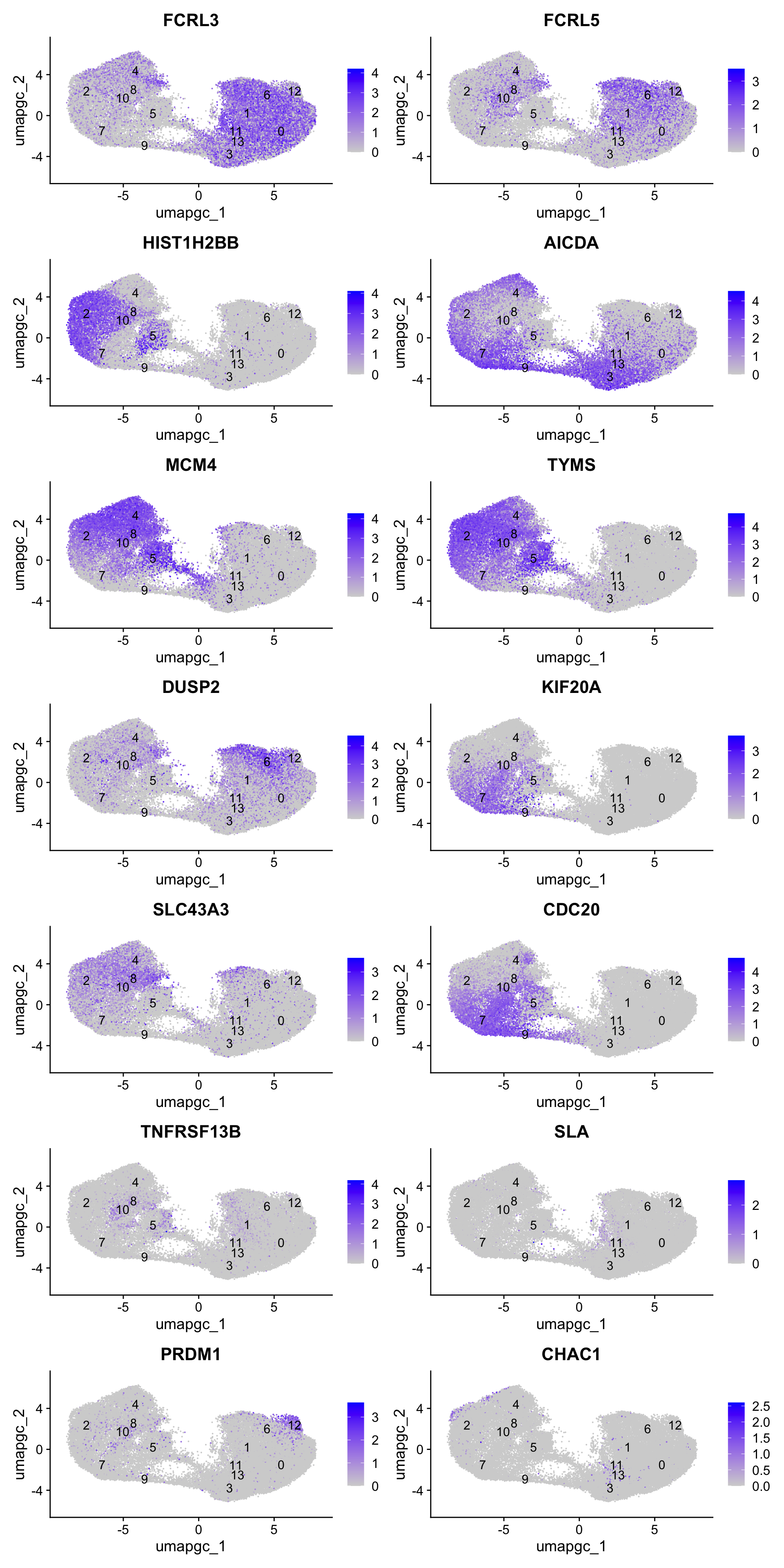
Top 10 marker genes from Seurat
## Seurat top markers
top10 <- paed_gc.markers %>%
    group_by(cluster) %>%
    top_n(n = 10, wt = avg_log2FC) %>%
    ungroup() %>%
    distinct(gene, .keep_all = TRUE) %>%
    arrange(cluster, desc(avg_log2FC))

cluster_colors <- paletteer::paletteer_d("pals::glasbey")[factor(top10$cluster)]

DotPlot(paed_gc,
        features = unique(top10$gene),
        group.by = opt_res,
        cols = c("azure1", "blueviolet"),
        dot.scale = 3, assay = "RNA") +
    RotatedAxis() +
    FontSize(y.text = 8, x.text = 12) +
    labs(y = element_blank(), x = element_blank()) +
    coord_flip() +
    theme(axis.text.y = element_text(color = cluster_colors)) +
    ggtitle("Top 10 marker genes per cluster (Seurat)")
Warning: Vectorized input to `element_text()` is not officially supported.
ℹ Results may be unexpected or may change in future versions of ggplot2.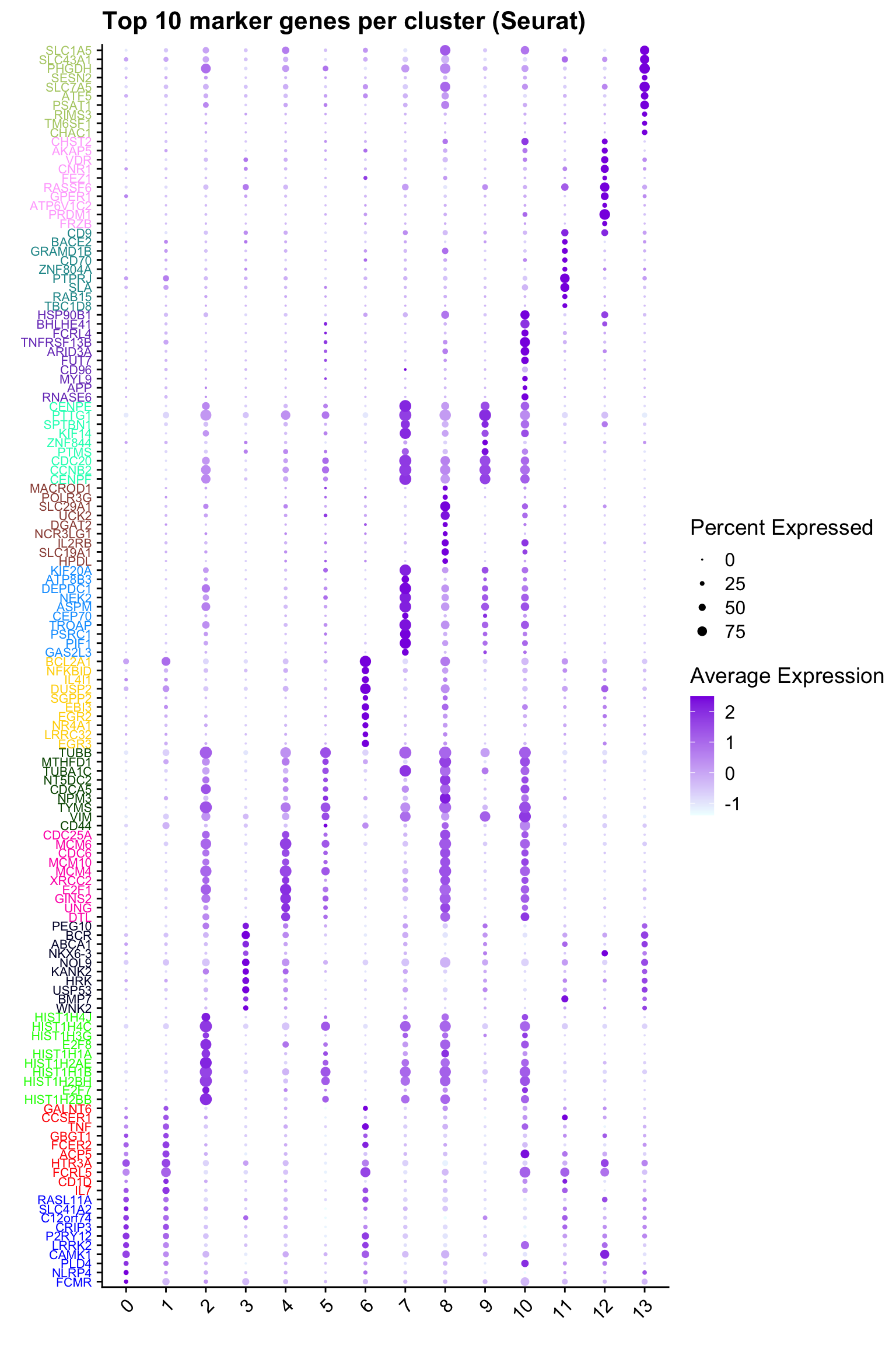
out_markers <- here("output",
            "CSV_v2",tissue,
            paste(tissue,"_Marker_genes_Reclustered_GC_population.",opt_res, sep = ""))

dir.create(out_markers, recursive = TRUE, showWarnings = FALSE)

for (cl in unique(paed_gc.markers$cluster)) {
  cluster_data <- paed_gc.markers %>% dplyr::filter(cluster == cl)
  file_name <- here(out_markers, paste0("G000231_Neeland_",tissue, "_cluster_", cl, ".csv"))
  if (!file.exists(file_name)) {
  write.csv(cluster_data, file = file_name)
  }
}
Corresponding Azimuth labels (GC cell subsets)
## Level 1
DimPlot(paed_gc, reduction = "umap.gc", group.by = "predicted.celltype.l1", raster = FALSE, repel = TRUE, label = TRUE, label.size = 4.5) 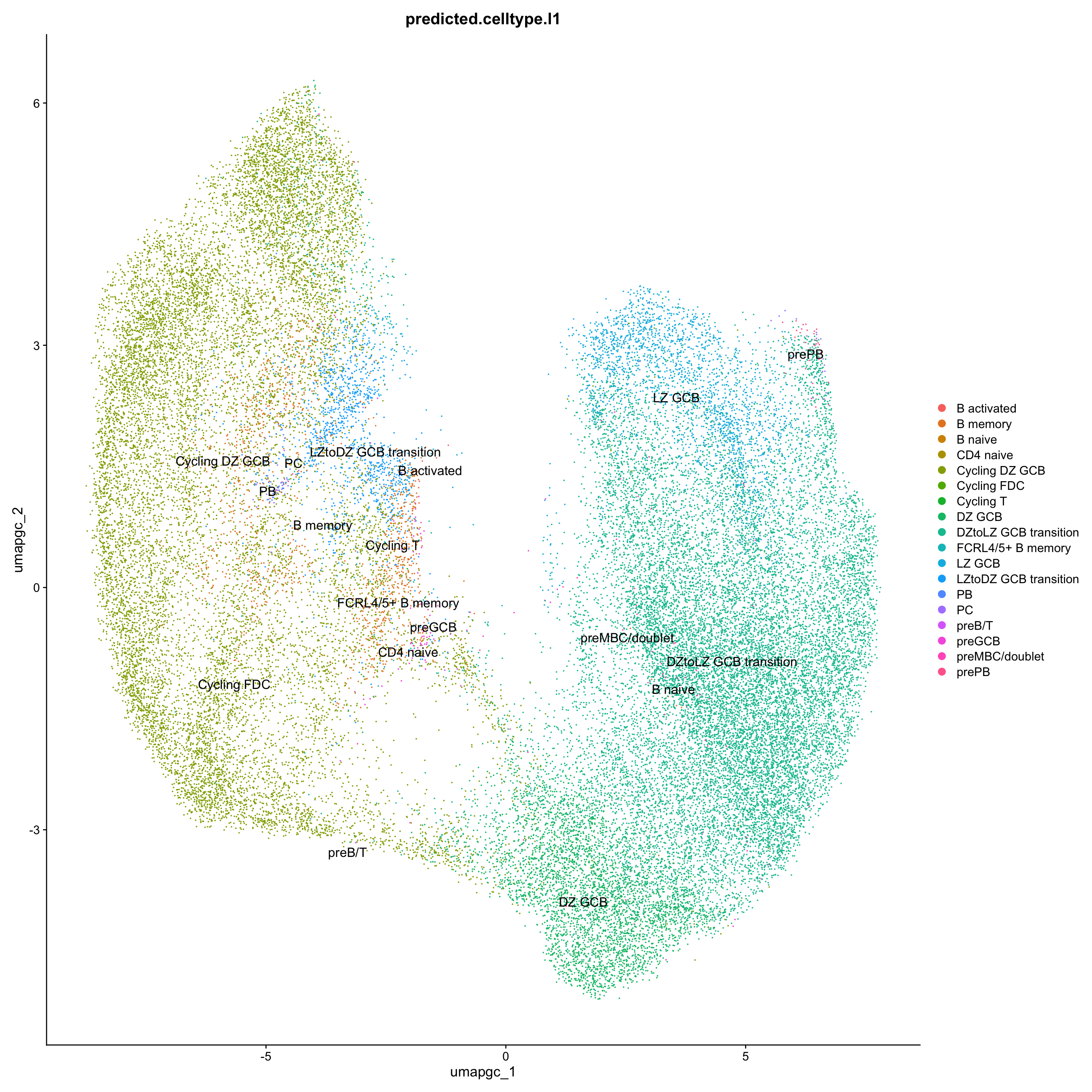
df_table <- as.data.frame(table(paed_gc$RNA_snn_res.0.6, paed_gc$predicted.celltype.l1))
ggplot(df_table, aes(Var1, Freq, fill = Var2)) +
  geom_bar(stat = "identity") +
  labs(x = "RNA_snn_res.0.6", y = "Count", fill = "predicted.celltype.l1") +
  theme_minimal() +
  ggtitle("Stacked Bar Plot of Tcell subsets (res=0.6) and predicted.celltype.l1")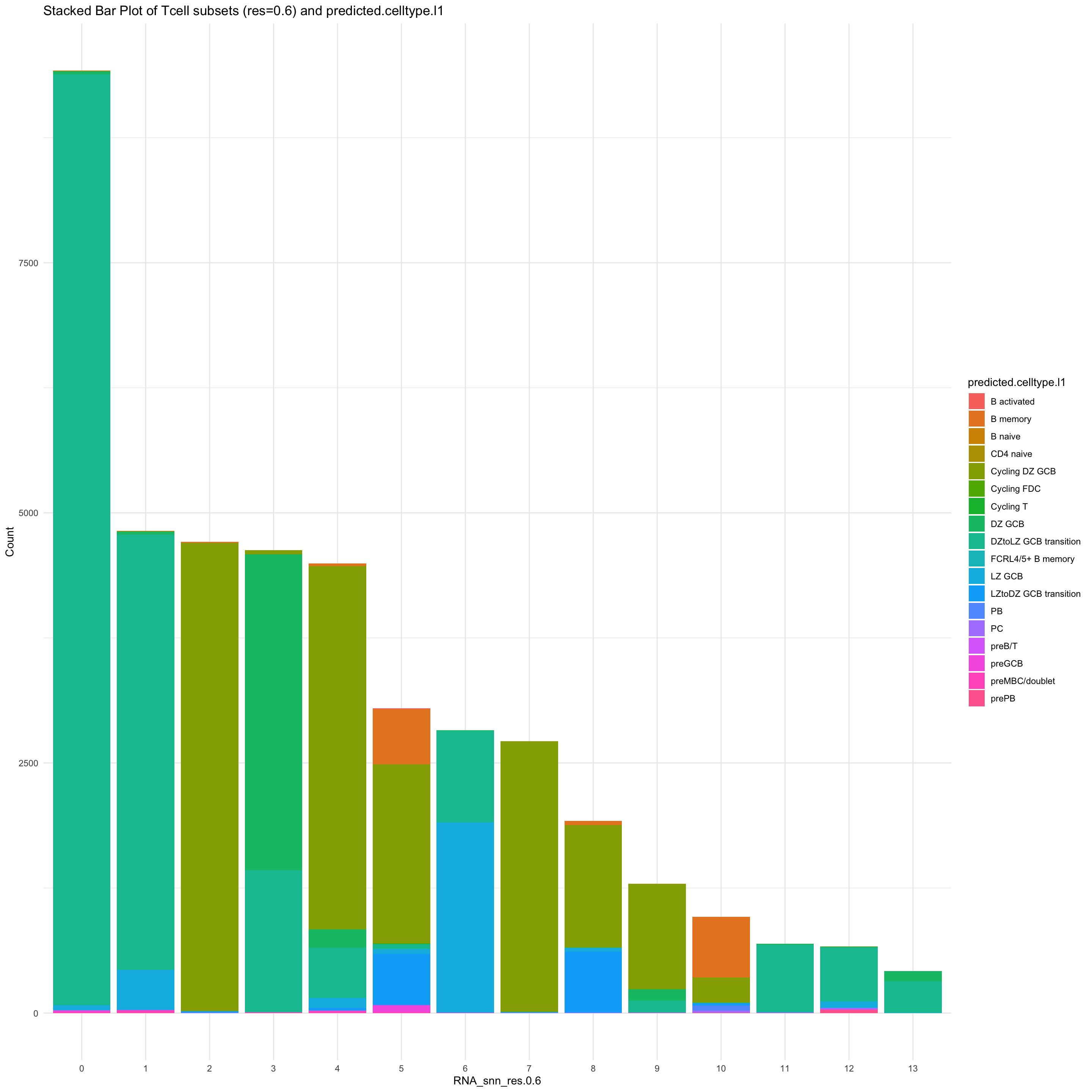
palette1 <- paletteer::paletteer_d("ggthemes::Classic_20")
palette2 <- paletteer::paletteer_d("Polychrome::light")
combined_palette <- unique(c(palette1, palette2))

labels <- "RNA_snn_res.0.6"

p <- vector("list",length(labels))
for(label in labels){
  paed_gc@meta.data %>%
    ggplot(aes(x = !!sym(label),
               fill = !!sym(label))) +
    geom_bar() +
    geom_text(aes(label = ..count..), stat = "count",
              vjust = -0.5, colour = "black", size = 2) +
    scale_y_log10() +
    theme(axis.text.x = element_blank(),
          axis.title.x = element_blank(),
          axis.ticks.x = element_blank()) +
    NoLegend() +
    labs(y = "No. Cells (log scale)") -> p1

  paed_gc@meta.data %>%
    dplyr::select(!!sym(label), donor_id) %>%
    group_by(!!sym(label), donor_id) %>%
    summarise(num = n()) %>%
    mutate(prop = num / sum(num)) %>%
  ggplot(aes(x = !!sym(label), y = prop * 100,
             fill = donor_id)) +
    geom_bar(stat = "identity") +
    theme(axis.text.x = element_text(angle = 90,
                                     vjust = 0.5,
                                     hjust = 1,
                                     size = 8)) +
    labs(y = "% Cells", fill = "Donor") +
  scale_fill_manual(values = combined_palette) -> p2

  (p1 / p2) & theme(legend.text = element_text(size = 8),
                  legend.key.size = unit(3, "mm")) -> p[[label]]
}
`summarise()` has grouped output by 'RNA_snn_res.0.6'. You can override using
the `.groups` argument.p[[1]]
NULL
$RNA_snn_res.0.6
| Version | Author | Date |
|---|---|---|
| 54e4ec2 | Gunjan Dixit | 2025-01-08 |
Old data- cells from previous clusters higlighted
Loading old Subclustering seurat object of T cell population and comparing with the updated clustering.
out2 <- here("output",
            "RDS", "AllBatches_Subclustering_SEUs", tissue,
             paste0("G000231_Neeland_",tissue,".GC_population.subclusters.SEU.rds"))

old_obj <- readRDS(out2)
cell_types <- unique(old_obj$cell_labels_v2)
for (cell_type in cell_types) {
cl_cells <- WhichCells(old_obj, idents = cell_type)
p <- DimPlot(
paed_gc,
reduction = "umap.gc",
label = TRUE,
label.size = 4.5,
repel = TRUE,
raster = FALSE,
cells.highlight = cl_cells
) +
ggtitle(paste("Updated- Highlighted:", cell_type))
p1 <- DimPlot(
old_obj,
reduction = "umap.new",
label = T,
label.size = 4.5,
repel = TRUE,
raster = FALSE,
cells.highlight = cl_cells
) +
ggtitle(paste("Old Data- Highlighted:", cell_type))
print(p | p1)
}
| Version | Author | Date |
|---|---|---|
| 54e4ec2 | Gunjan Dixit | 2025-01-08 |
| Version | Author | Date |
|---|---|---|
| 54e4ec2 | Gunjan Dixit | 2025-01-08 |
| Version | Author | Date |
|---|---|---|
| 54e4ec2 | Gunjan Dixit | 2025-01-08 |
| Version | Author | Date |
|---|---|---|
| 54e4ec2 | Gunjan Dixit | 2025-01-08 |
| Version | Author | Date |
|---|---|---|
| 54e4ec2 | Gunjan Dixit | 2025-01-08 |
| Version | Author | Date |
|---|---|---|
| 54e4ec2 | Gunjan Dixit | 2025-01-08 |
| Version | Author | Date |
|---|---|---|
| 54e4ec2 | Gunjan Dixit | 2025-01-08 |
| Version | Author | Date |
|---|---|---|
| 54e4ec2 | Gunjan Dixit | 2025-01-08 |
| Version | Author | Date |
|---|---|---|
| 54e4ec2 | Gunjan Dixit | 2025-01-08 |
| Version | Author | Date |
|---|---|---|
| 54e4ec2 | Gunjan Dixit | 2025-01-08 |
| Version | Author | Date |
|---|---|---|
| 54e4ec2 | Gunjan Dixit | 2025-01-08 |
| Version | Author | Date |
|---|---|---|
| 54e4ec2 | Gunjan Dixit | 2025-01-08 |
Save subclustered SEU object
out2 <- here("output",
            "RDS", "AllBatches_Subclustering_SEUs_v2", tissue,
             paste0("G000231_Neeland_",tissue,".GC_population.subclusters.SEU.rds"))
#dir.create(out2)
#if (!file.exists(out2)) {
  saveRDS(paed_gc, file = out2)
#}
Updated cell-type labels (GC cell clusters)
cell_labels <- readxl::read_excel(here("data/cell_labels_Mel_v4_Dec2024/earlyAIR_Adenoids_all.xlsx"), sheet = "GC-B reclustering")

new_cluster_names <- cell_labels %>%
  dplyr::select(cluster, annotation) %>%
  deframe()

paed_gc <- RenameIdents(paed_gc, new_cluster_names)
paed_gc@meta.data$cell_labels_v2 <- Idents(paed_gc)

p3 <- DimPlot(paed_gc, reduction = "umap.gc", raster = FALSE, repel = TRUE, label = TRUE, label.size = 3.5) + ggtitle(paste0(tissue, ": UMAP with Updated GC cell population"))

p3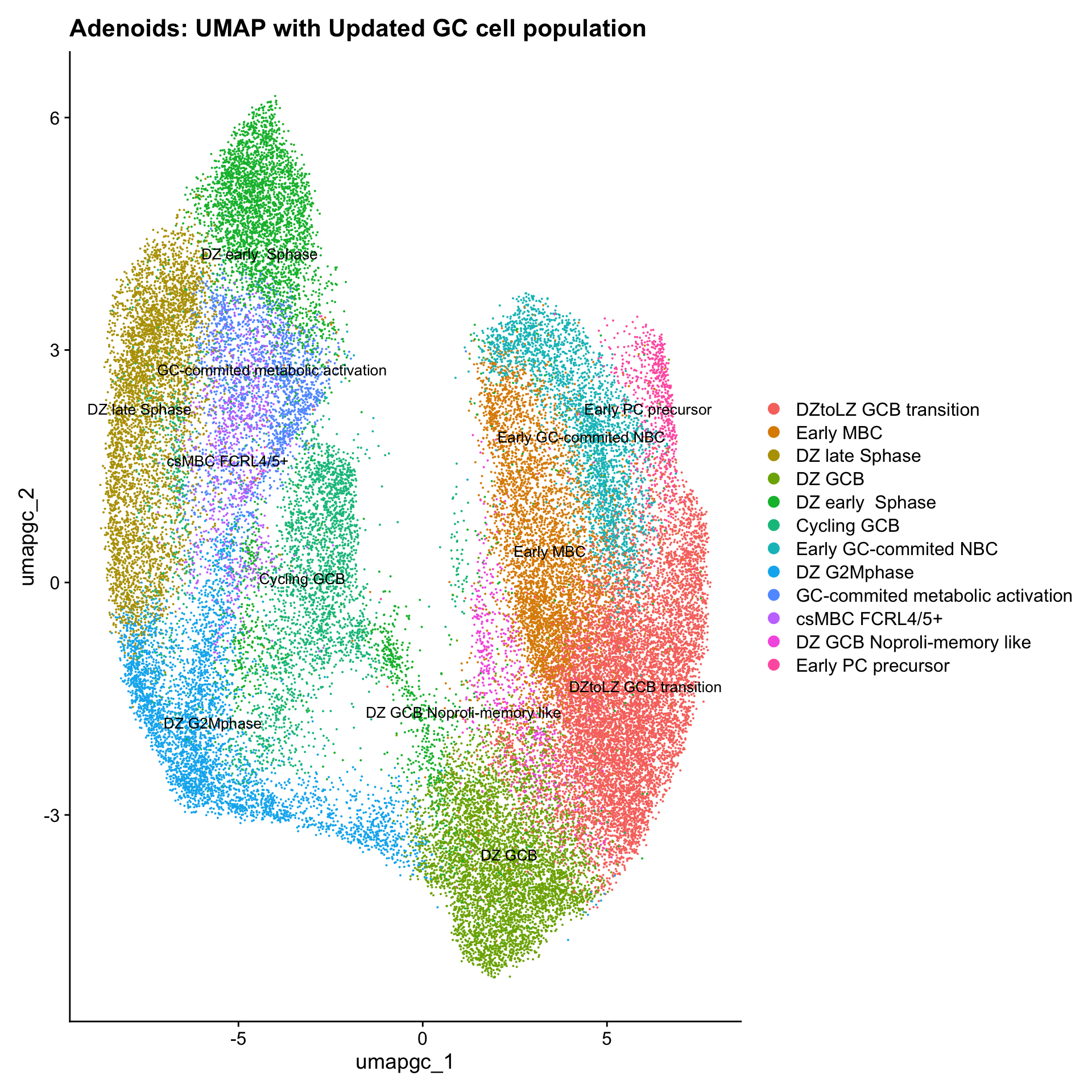
| Version | Author | Date |
|---|---|---|
| 54e4ec2 | Gunjan Dixit | 2025-01-08 |
Save subclustered SEU object Germinal Centre Bcells
out2 <- here("output",
            "RDS", "AllBatches_Annotated_Subclustering_SEUs_v2", tissue,
             paste0("G000231_Neeland_",tissue,".GC_population.subclusters.SEU.rds"))
#dir.create(out2)
if (!file.exists(out2)) {
  saveRDS(paed_gc, file = out2)
}
Other Clusters (excluding subclusters)
idx <- which(Idents(merged_obj) %in% c("T cells for reclustering", "Germinal centre B cells for reclustering"))
paed_other <- merged_obj[,-idx]
paed_other
An object of class Seurat
17456 features across 89157 samples within 1 assay
Active assay: RNA (17456 features, 2000 variable features)
3 layers present: data, counts, scale.data
4 dimensional reductions calculated: pca, umap.unintegrated, harmony, umap.harmonySave subclustered SEU object ( All other cells)
paed_other$cell_labels_v2 <-paed_other$cell_labels
out2 <- here("output",
            "RDS", "AllBatches_Annotated_Subclustering_SEUs_v2", tissue,
             paste0("G000231_Neeland_",tissue,".all_other.subclusters.SEU.rds"))

if (!file.exists(out2)) {
  saveRDS(paed_other, file = out2)
}
Merge seurat objects of subclusters
files <- list.files(here("output",
            "RDS", "AllBatches_Annotated_Subclustering_SEUs_v2", tissue),
                    full.names = TRUE)

seuLst <- lapply(files, function(f) readRDS(f))

seu <- merge(seuLst[[1]],
             y = c(seuLst[[2]],
                   seuLst[[3]]))
seu
An object of class Seurat
17456 features across 184005 samples within 1 assay
Active assay: RNA (17456 features, 2000 variable features)
9 layers present: data.1, data.2, data.3, counts.1, scale.data.1, counts.2, scale.data.2, counts.3, scale.data.3merged <- seu %>%
NormalizeData() %>%
FindVariableFeatures() %>%
ScaleData() %>%
RunPCA()Normalizing layer: counts.1Normalizing layer: counts.2Normalizing layer: counts.3Finding variable features for layer counts.1Finding variable features for layer counts.2Finding variable features for layer counts.3Centering and scaling data matrixPC_ 1
Positive: MKI67, KIFC1, NUSAP1, CDK1, AURKB, TYMS, NCAPG, TK1, STMN1, TOP2A
TPX2, ZWINT, KIF11, HIST1H1B, FOXM1, RRM2, HJURP, BIRC5, HMGB2, ASF1B
KIF2C, MYBL2, CCNA2, CCNB2, SPC25, SHCBP1, CDCA8, MND1, UHRF1, ANLN
Negative: FCMR, TRBC2, SELL, PLAC8, KLF2, CD69, DUSP1, GPR183, TCF7, CCR6
LY6E, JUN, CCR7, JUNB, IL32, DDIT4, LCP2, PLAAT4, TC2N, RIN3
IL7R, MPEG1, ARL4C, TRBC1, SAMD9L, CTSB, IFI44, AHNAK, CD4, IFI44L
PC_ 2
Positive: CD79A, MS4A1, CD22, CD79B, PAX5, IGHM, IGHD, FCRL1, CD72, BCL11A
CD74, CIITA, TCL1A, CD83, NIBAN3, IGKC, FCRLA, CR1, POU2AF1, PHACTR1
FCRL5, CCR6, ADAM19, MARCKSL1, FCRL3, VPREB3, RUBCNL, FAM30A, SPIB, CXCR5
Negative: LGALS3, SDC4, ANXA1, EHF, IFI27, CDH1, KIAA1522, ALDH1A1, ATP1B1, MYO5B
CST3, TNFRSF21, PTPRF, CFB, ALDH3B1, IGFBP2, MAL2, PERP, IGFBP7, GOLM1
NUPR1, EPHX1, CLDN4, TNFAIP2, ELF3, EMP2, MUC1, WFDC2, PARVA, S100A11
PC_ 3
Positive: IL32, TCF7, LCP2, TRBC1, MAF, CD4, SRGN, IL2RB, ITM2A, TC2N
SPN, ICOS, TIGIT, SH2D1A, TRBC2, IL7R, PYHIN1, TOX2, IL6R, PDCD1
HNRNPLL, TBC1D4, ZNRF1, CTLA4, PLAAT4, LEF1, ACTN1, ATP2B4, GBP2, FKBP5
Negative: CD79A, MS4A1, CD74, CD22, CD79B, CIITA, PAX5, IGHM, BCL11A, FCRL1
CD72, IGHD, CD83, IFI30, NIBAN3, CD24, IGKC, PHACTR1, FCRL5, CR1
TCL1A, FCRLA, MPEG1, ADAM19, CCR6, SPIB, FCRL3, UNC93B1, POU2AF1, RUBCNL
PC_ 4
Positive: TRBC2, TCF7, TC2N, ITM2A, TRBC1, IL32, FCMR, ICOS, TIGIT, PYHIN1
IKZF3, TOX2, SH2D1A, MAF, PDCD1, SYNE2, LEF1, PLAAT4, KIAA1671, CXCR5
CAPS, IL7R, CCR7, PIM2, DTHD1, EPPK1, GRAP2, SARDH, AQP3, CFAP73
Negative: LYZ, FCER1G, CST3, MS4A6A, TYROBP, CSF1R, CD68, TMEM176B, SERPINA1, ENPP2
HCK, SLC8A1, SERPINF1, ITGAX, KCTD12, MAFB, CD14, TNFAIP2, TMEM176A, GSN
GRN, CMKLR1, CD300LF, PLA2G7, CPVL, LGALS1, IL18, CEBPD, LILRB2, AIF1
PC_ 5
Positive: KIF20A, PSRC1, CENPA, PLK1, KIF14, NEK2, CENPE, ASPM, HMMR, TROAP
CDC20, DLGAP5, KIF23, AURKA, DEPDC1, PIF1, CDCA8, CENPF, GTSE1, CCNB2
FAM83D, CDCA3, HJURP, CKAP2L, TOP2A, UBE2C, NUF2, KIF18B, SGO2, BUB1
Negative: MEF2B, SLBP, GINS2, MCM4, RGS13, E2F1, BCL6, MCM6, LHFPL2, LMO2
CDC6, HELLS, UNG, SYNE2, NME1, DTL, WDR76, CAMK1, PKM, DHRS9
BCAT1, CCNE2, DUSP2, ENO1, ODC1, EIF4A1, MCM10, PRMT1, MARCKSL1, HMCES merged <- RunUMAP(merged, dims = 1:30, reduction = "pca", reduction.name = "umap.merged")16:46:44 UMAP embedding parameters a = 0.9922 b = 1.11216:46:44 Read 184005 rows and found 30 numeric columns16:46:44 Using Annoy for neighbor search, n_neighbors = 3016:46:44 Building Annoy index with metric = cosine, n_trees = 500% 10 20 30 40 50 60 70 80 90 100%[----|----|----|----|----|----|----|----|----|----|**************************************************|
16:46:54 Writing NN index file to temp file /var/folders/q8/kw1r78g12qn793xm7g0zvk94x2bh70/T//Rtmpgzvl9C/file36db1ffe381c
16:46:54 Searching Annoy index using 1 thread, search_k = 3000
16:47:33 Annoy recall = 100%
16:47:34 Commencing smooth kNN distance calibration using 1 thread with target n_neighbors = 30
16:47:36 Initializing from normalized Laplacian + noise (using RSpectra)
16:48:04 Commencing optimization for 200 epochs, with 8231698 positive edges
16:48:51 Optimization finishedp4 <- DimPlot(merged, reduction = "umap.merged", group.by = "cell_labels_v2",raster = FALSE, repel = TRUE, label = TRUE, label.size = 4.5) + ggtitle(paste0(tissue, ": UMAP with annotations")) + NoLegend()
p4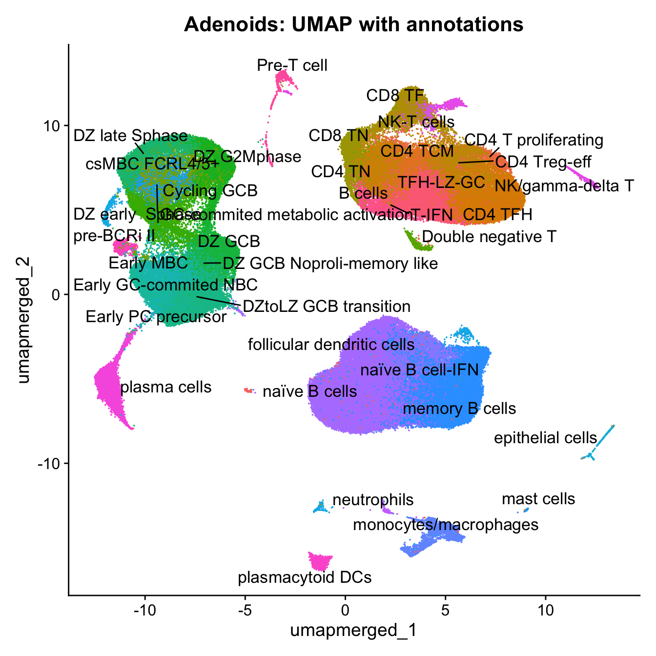
Save Final SEU object (All cells)
out3 <- here("output",
            "RDS", "AllBatches_Final_Clusters_SEUs_v2",
             paste0("G000231_Neeland_",tissue,".final_clusters.SEU.rds"))

#if (!file.exists(out3)) {
  saveRDS(merged, file = out3)
#}
labels <- c("cell_labels", "cell_labels_v2")
p <- vector("list",length(labels))
for(label in labels){
merged@meta.data %>%
ggplot(aes(x = !!sym(label),
fill = !!sym(label))) +
geom_bar() +
geom_text(aes(label = ..count..), stat = "count",
vjust = -0.5, colour = "black", size = 2) +
scale_y_log10() +
theme(axis.text.x = element_blank(),
axis.title.x = element_blank(),
axis.ticks.x = element_blank()) +
NoLegend() +
labs(y = "No. Cells (log scale)") -> p1
merged@meta.data %>%
dplyr::select(!!sym(label), donor_id) %>%
group_by(!!sym(label), donor_id) %>%
summarise(num = n()) %>%
mutate(prop = num / sum(num)) %>%
ggplot(aes(x = !!sym(label), y = prop * 100,
fill = donor_id)) +
geom_bar(stat = "identity") +
theme(axis.text.x = element_text(angle = 90,
vjust = 0.5,
hjust = 1,
size = 8)) +
labs(y = "% Cells", fill = "Donor") +
scale_fill_manual(values = combined_palette) -> p2
(p1 / p2) & theme(legend.text = element_text(size = 8),
legend.key.size = unit(3, "mm")) -> p[[label]]
}`summarise()` has grouped output by 'cell_labels'. You can override using the
`.groups` argument.
`summarise()` has grouped output by 'cell_labels_v2'. You can override using
the `.groups` argument.p[[1]]
NULL
[[2]]
NULL
$cell_labels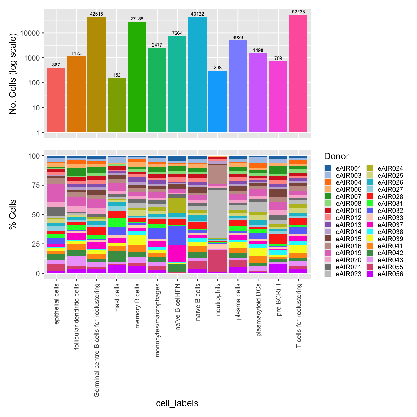
$cell_labels_v2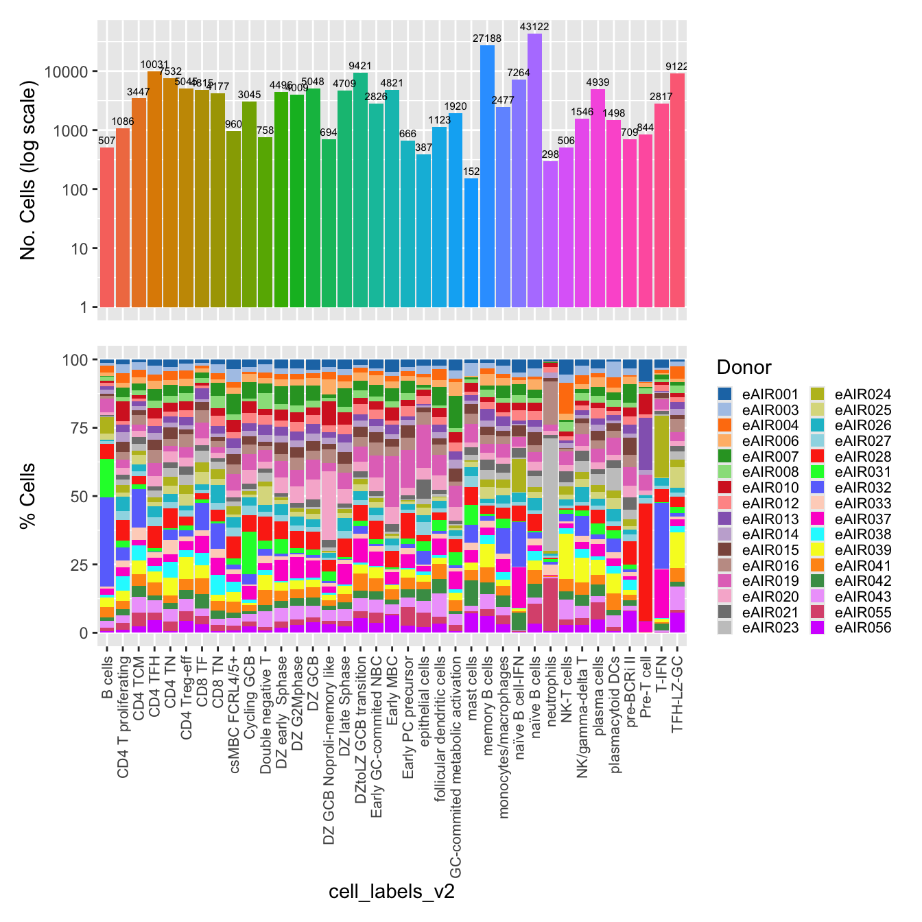
Session Info
sessioninfo::session_info()─ Session info ───────────────────────────────────────────────────────────────
setting value
version R version 4.3.2 (2023-10-31)
os macOS 15.2
system aarch64, darwin20
ui X11
language (EN)
collate en_US.UTF-8
ctype en_US.UTF-8
tz Australia/Melbourne
date 2025-01-16
pandoc 3.1.1 @ /Users/dixitgunjan/Desktop/RStudio.app/Contents/Resources/app/quarto/bin/tools/ (via rmarkdown)
─ Packages ───────────────────────────────────────────────────────────────────
package * version date (UTC) lib source
abind 1.4-5 2016-07-21 [1] CRAN (R 4.3.0)
backports 1.4.1 2021-12-13 [1] CRAN (R 4.3.0)
beeswarm 0.4.0 2021-06-01 [1] CRAN (R 4.3.0)
BiocManager 1.30.22 2023-08-08 [1] CRAN (R 4.3.0)
BiocStyle * 2.30.0 2023-10-26 [1] Bioconductor
bslib 0.6.1 2023-11-28 [1] CRAN (R 4.3.1)
cachem 1.0.8 2023-05-01 [1] CRAN (R 4.3.0)
callr 3.7.5 2024-02-19 [1] CRAN (R 4.3.1)
cellranger 1.1.0 2016-07-27 [1] CRAN (R 4.3.0)
checkmate 2.3.1 2023-12-04 [1] CRAN (R 4.3.1)
cli 3.6.2 2023-12-11 [1] CRAN (R 4.3.1)
cluster 2.1.6 2023-12-01 [1] CRAN (R 4.3.1)
clustree * 0.5.1 2023-11-05 [1] CRAN (R 4.3.1)
codetools 0.2-19 2023-02-01 [1] CRAN (R 4.3.2)
colorspace 2.1-0 2023-01-23 [1] CRAN (R 4.3.0)
cowplot 1.1.3 2024-01-22 [1] CRAN (R 4.3.1)
data.table * 1.15.0 2024-01-30 [1] CRAN (R 4.3.1)
deldir 2.0-2 2023-11-23 [1] CRAN (R 4.3.1)
digest 0.6.34 2024-01-11 [1] CRAN (R 4.3.1)
dotCall64 1.1-1 2023-11-28 [1] CRAN (R 4.3.1)
dplyr * 1.1.4 2023-11-17 [1] CRAN (R 4.3.1)
ellipsis 0.3.2 2021-04-29 [1] CRAN (R 4.3.0)
evaluate 0.23 2023-11-01 [1] CRAN (R 4.3.1)
fansi 1.0.6 2023-12-08 [1] CRAN (R 4.3.1)
farver 2.1.1 2022-07-06 [1] CRAN (R 4.3.0)
fastDummies 1.7.3 2023-07-06 [1] CRAN (R 4.3.0)
fastmap 1.1.1 2023-02-24 [1] CRAN (R 4.3.0)
fitdistrplus 1.1-11 2023-04-25 [1] CRAN (R 4.3.0)
forcats * 1.0.0 2023-01-29 [1] CRAN (R 4.3.0)
fs 1.6.3 2023-07-20 [1] CRAN (R 4.3.0)
future 1.33.1 2023-12-22 [1] CRAN (R 4.3.1)
future.apply 1.11.1 2023-12-21 [1] CRAN (R 4.3.1)
generics 0.1.3 2022-07-05 [1] CRAN (R 4.3.0)
getPass 0.2-4 2023-12-10 [1] CRAN (R 4.3.1)
ggbeeswarm 0.7.2 2023-04-29 [1] CRAN (R 4.3.0)
ggforce 0.4.2 2024-02-19 [1] CRAN (R 4.3.1)
ggplot2 * 3.5.0 2024-02-23 [1] CRAN (R 4.3.1)
ggraph * 2.1.0 2022-10-09 [1] CRAN (R 4.3.0)
ggrastr 1.0.2 2023-06-01 [1] CRAN (R 4.3.0)
ggrepel 0.9.5 2024-01-10 [1] CRAN (R 4.3.1)
ggridges 0.5.6 2024-01-23 [1] CRAN (R 4.3.1)
git2r 0.33.0 2023-11-26 [1] CRAN (R 4.3.1)
globals 0.16.2 2022-11-21 [1] CRAN (R 4.3.0)
glue 1.7.0 2024-01-09 [1] CRAN (R 4.3.1)
goftest 1.2-3 2021-10-07 [1] CRAN (R 4.3.0)
graphlayouts 1.1.0 2024-01-19 [1] CRAN (R 4.3.1)
gridExtra 2.3 2017-09-09 [1] CRAN (R 4.3.0)
gtable 0.3.4 2023-08-21 [1] CRAN (R 4.3.0)
here * 1.0.1 2020-12-13 [1] CRAN (R 4.3.0)
highr 0.10 2022-12-22 [1] CRAN (R 4.3.0)
hms 1.1.3 2023-03-21 [1] CRAN (R 4.3.0)
htmltools 0.5.7 2023-11-03 [1] CRAN (R 4.3.1)
htmlwidgets 1.6.4 2023-12-06 [1] CRAN (R 4.3.1)
httpuv 1.6.14 2024-01-26 [1] CRAN (R 4.3.1)
httr 1.4.7 2023-08-15 [1] CRAN (R 4.3.0)
ica 1.0-3 2022-07-08 [1] CRAN (R 4.3.0)
igraph 2.0.2 2024-02-17 [1] CRAN (R 4.3.1)
irlba 2.3.5.1 2022-10-03 [1] CRAN (R 4.3.2)
jquerylib 0.1.4 2021-04-26 [1] CRAN (R 4.3.0)
jsonlite 1.8.8 2023-12-04 [1] CRAN (R 4.3.1)
kableExtra * 1.4.0 2024-01-24 [1] CRAN (R 4.3.1)
KernSmooth 2.23-22 2023-07-10 [1] CRAN (R 4.3.2)
knitr 1.45 2023-10-30 [1] CRAN (R 4.3.1)
labeling 0.4.3 2023-08-29 [1] CRAN (R 4.3.0)
later 1.3.2 2023-12-06 [1] CRAN (R 4.3.1)
lattice 0.22-5 2023-10-24 [1] CRAN (R 4.3.1)
lazyeval 0.2.2 2019-03-15 [1] CRAN (R 4.3.0)
leiden 0.4.3.1 2023-11-17 [1] CRAN (R 4.3.1)
lifecycle 1.0.4 2023-11-07 [1] CRAN (R 4.3.1)
limma 3.58.1 2023-11-02 [1] Bioconductor
listenv 0.9.1 2024-01-29 [1] CRAN (R 4.3.1)
lmtest 0.9-40 2022-03-21 [1] CRAN (R 4.3.0)
lubridate * 1.9.3 2023-09-27 [1] CRAN (R 4.3.1)
magrittr 2.0.3 2022-03-30 [1] CRAN (R 4.3.0)
MASS 7.3-60.0.1 2024-01-13 [1] CRAN (R 4.3.1)
Matrix 1.6-5 2024-01-11 [1] CRAN (R 4.3.1)
matrixStats 1.2.0 2023-12-11 [1] CRAN (R 4.3.1)
mime 0.12 2021-09-28 [1] CRAN (R 4.3.0)
miniUI 0.1.1.1 2018-05-18 [1] CRAN (R 4.3.0)
munsell 0.5.0 2018-06-12 [1] CRAN (R 4.3.0)
nlme 3.1-164 2023-11-27 [1] CRAN (R 4.3.1)
paletteer 1.6.0 2024-01-21 [1] CRAN (R 4.3.1)
parallelly 1.37.0 2024-02-14 [1] CRAN (R 4.3.1)
patchwork * 1.2.0 2024-01-08 [1] CRAN (R 4.3.1)
pbapply 1.7-2 2023-06-27 [1] CRAN (R 4.3.0)
pillar 1.9.0 2023-03-22 [1] CRAN (R 4.3.0)
pkgconfig 2.0.3 2019-09-22 [1] CRAN (R 4.3.0)
plotly 4.10.4 2024-01-13 [1] CRAN (R 4.3.1)
plyr 1.8.9 2023-10-02 [1] CRAN (R 4.3.1)
png 0.1-8 2022-11-29 [1] CRAN (R 4.3.0)
polyclip 1.10-6 2023-09-27 [1] CRAN (R 4.3.1)
presto 1.0.0 2024-02-27 [1] Github (immunogenomics/presto@31dc97f)
prismatic 1.1.1 2022-08-15 [1] CRAN (R 4.3.0)
processx 3.8.3 2023-12-10 [1] CRAN (R 4.3.1)
progressr 0.14.0 2023-08-10 [1] CRAN (R 4.3.0)
promises 1.2.1 2023-08-10 [1] CRAN (R 4.3.0)
ps 1.7.6 2024-01-18 [1] CRAN (R 4.3.1)
purrr * 1.0.2 2023-08-10 [1] CRAN (R 4.3.0)
R6 2.5.1 2021-08-19 [1] CRAN (R 4.3.0)
RANN 2.6.1 2019-01-08 [1] CRAN (R 4.3.0)
RColorBrewer * 1.1-3 2022-04-03 [1] CRAN (R 4.3.0)
Rcpp 1.0.12 2024-01-09 [1] CRAN (R 4.3.1)
RcppAnnoy 0.0.22 2024-01-23 [1] CRAN (R 4.3.1)
RcppHNSW 0.6.0 2024-02-04 [1] CRAN (R 4.3.1)
readr * 2.1.5 2024-01-10 [1] CRAN (R 4.3.1)
readxl * 1.4.3 2023-07-06 [1] CRAN (R 4.3.0)
rematch2 2.1.2 2020-05-01 [1] CRAN (R 4.3.0)
reshape2 1.4.4 2020-04-09 [1] CRAN (R 4.3.0)
reticulate 1.35.0 2024-01-31 [1] CRAN (R 4.3.1)
rlang 1.1.3 2024-01-10 [1] CRAN (R 4.3.1)
rmarkdown 2.25 2023-09-18 [1] CRAN (R 4.3.1)
ROCR 1.0-11 2020-05-02 [1] CRAN (R 4.3.0)
rprojroot 2.0.4 2023-11-05 [1] CRAN (R 4.3.1)
RSpectra 0.16-1 2022-04-24 [1] CRAN (R 4.3.0)
rstudioapi 0.15.0 2023-07-07 [1] CRAN (R 4.3.0)
Rtsne 0.17 2023-12-07 [1] CRAN (R 4.3.1)
sass 0.4.8 2023-12-06 [1] CRAN (R 4.3.1)
scales 1.3.0 2023-11-28 [1] CRAN (R 4.3.1)
scattermore 1.2 2023-06-12 [1] CRAN (R 4.3.0)
sctransform 0.4.1 2023-10-19 [1] CRAN (R 4.3.1)
sessioninfo 1.2.2 2021-12-06 [1] CRAN (R 4.3.0)
Seurat * 5.0.1.9009 2024-02-28 [1] Github (satijalab/seurat@6a3ef5e)
SeuratObject * 5.0.1 2023-11-17 [1] CRAN (R 4.3.1)
shiny 1.8.0 2023-11-17 [1] CRAN (R 4.3.1)
sp * 2.1-3 2024-01-30 [1] CRAN (R 4.3.1)
spam 2.10-0 2023-10-23 [1] CRAN (R 4.3.1)
spatstat.data 3.0-4 2024-01-15 [1] CRAN (R 4.3.1)
spatstat.explore 3.2-6 2024-02-01 [1] CRAN (R 4.3.1)
spatstat.geom 3.2-8 2024-01-26 [1] CRAN (R 4.3.1)
spatstat.random 3.2-2 2023-11-29 [1] CRAN (R 4.3.1)
spatstat.sparse 3.0-3 2023-10-24 [1] CRAN (R 4.3.1)
spatstat.utils 3.0-4 2023-10-24 [1] CRAN (R 4.3.1)
statmod 1.5.0 2023-01-06 [1] CRAN (R 4.3.0)
stringi 1.8.3 2023-12-11 [1] CRAN (R 4.3.1)
stringr * 1.5.1 2023-11-14 [1] CRAN (R 4.3.1)
survival 3.5-8 2024-02-14 [1] CRAN (R 4.3.1)
svglite 2.1.3 2023-12-08 [1] CRAN (R 4.3.1)
systemfonts 1.0.5 2023-10-09 [1] CRAN (R 4.3.1)
tensor 1.5 2012-05-05 [1] CRAN (R 4.3.0)
tibble * 3.2.1 2023-03-20 [1] CRAN (R 4.3.0)
tidygraph 1.3.1 2024-01-30 [1] CRAN (R 4.3.1)
tidyr * 1.3.1 2024-01-24 [1] CRAN (R 4.3.1)
tidyselect 1.2.0 2022-10-10 [1] CRAN (R 4.3.0)
tidyverse * 2.0.0 2023-02-22 [1] CRAN (R 4.3.0)
timechange 0.3.0 2024-01-18 [1] CRAN (R 4.3.1)
tweenr 2.0.3 2024-02-26 [1] CRAN (R 4.3.1)
tzdb 0.4.0 2023-05-12 [1] CRAN (R 4.3.0)
utf8 1.2.4 2023-10-22 [1] CRAN (R 4.3.1)
uwot 0.1.16 2023-06-29 [1] CRAN (R 4.3.0)
vctrs 0.6.5 2023-12-01 [1] CRAN (R 4.3.1)
vipor 0.4.7 2023-12-18 [1] CRAN (R 4.3.1)
viridis 0.6.5 2024-01-29 [1] CRAN (R 4.3.1)
viridisLite 0.4.2 2023-05-02 [1] CRAN (R 4.3.0)
whisker 0.4.1 2022-12-05 [1] CRAN (R 4.3.0)
withr 3.0.0 2024-01-16 [1] CRAN (R 4.3.1)
workflowr * 1.7.1 2023-08-23 [1] CRAN (R 4.3.0)
xfun 0.42 2024-02-08 [1] CRAN (R 4.3.1)
xml2 1.3.6 2023-12-04 [1] CRAN (R 4.3.1)
xtable 1.8-4 2019-04-21 [1] CRAN (R 4.3.0)
yaml 2.3.8 2023-12-11 [1] CRAN (R 4.3.1)
zoo 1.8-12 2023-04-13 [1] CRAN (R 4.3.0)
[1] /Library/Frameworks/R.framework/Versions/4.3-arm64/Resources/library
──────────────────────────────────────────────────────────────────────────────
sessionInfo()R version 4.3.2 (2023-10-31)
Platform: aarch64-apple-darwin20 (64-bit)
Running under: macOS 15.2
Matrix products: default
BLAS: /Library/Frameworks/R.framework/Versions/4.3-arm64/Resources/lib/libRblas.0.dylib
LAPACK: /Library/Frameworks/R.framework/Versions/4.3-arm64/Resources/lib/libRlapack.dylib; LAPACK version 3.11.0
locale:
[1] en_US.UTF-8/en_US.UTF-8/en_US.UTF-8/C/en_US.UTF-8/en_US.UTF-8
time zone: Australia/Melbourne
tzcode source: internal
attached base packages:
[1] stats graphics grDevices utils datasets methods base
other attached packages:
[1] readxl_1.4.3 patchwork_1.2.0 data.table_1.15.0 RColorBrewer_1.1-3
[5] kableExtra_1.4.0 clustree_0.5.1 ggraph_2.1.0 Seurat_5.0.1.9009
[9] SeuratObject_5.0.1 sp_2.1-3 here_1.0.1 lubridate_1.9.3
[13] forcats_1.0.0 stringr_1.5.1 dplyr_1.1.4 purrr_1.0.2
[17] readr_2.1.5 tidyr_1.3.1 tibble_3.2.1 ggplot2_3.5.0
[21] tidyverse_2.0.0 BiocStyle_2.30.0 workflowr_1.7.1
loaded via a namespace (and not attached):
[1] RcppAnnoy_0.0.22 splines_4.3.2 later_1.3.2
[4] prismatic_1.1.1 cellranger_1.1.0 polyclip_1.10-6
[7] fastDummies_1.7.3 lifecycle_1.0.4 rprojroot_2.0.4
[10] globals_0.16.2 processx_3.8.3 lattice_0.22-5
[13] MASS_7.3-60.0.1 backports_1.4.1 magrittr_2.0.3
[16] limma_3.58.1 plotly_4.10.4 sass_0.4.8
[19] rmarkdown_2.25 jquerylib_0.1.4 yaml_2.3.8
[22] httpuv_1.6.14 sctransform_0.4.1 spam_2.10-0
[25] sessioninfo_1.2.2 spatstat.sparse_3.0-3 reticulate_1.35.0
[28] cowplot_1.1.3 pbapply_1.7-2 abind_1.4-5
[31] Rtsne_0.17 presto_1.0.0 tweenr_2.0.3
[34] git2r_0.33.0 ggrepel_0.9.5 irlba_2.3.5.1
[37] listenv_0.9.1 spatstat.utils_3.0-4 goftest_1.2-3
[40] RSpectra_0.16-1 spatstat.random_3.2-2 fitdistrplus_1.1-11
[43] parallelly_1.37.0 svglite_2.1.3 leiden_0.4.3.1
[46] codetools_0.2-19 xml2_1.3.6 ggforce_0.4.2
[49] tidyselect_1.2.0 farver_2.1.1 viridis_0.6.5
[52] matrixStats_1.2.0 spatstat.explore_3.2-6 jsonlite_1.8.8
[55] ellipsis_0.3.2 tidygraph_1.3.1 progressr_0.14.0
[58] ggridges_0.5.6 survival_3.5-8 systemfonts_1.0.5
[61] tools_4.3.2 ica_1.0-3 Rcpp_1.0.12
[64] glue_1.7.0 gridExtra_2.3 xfun_0.42
[67] withr_3.0.0 BiocManager_1.30.22 fastmap_1.1.1
[70] fansi_1.0.6 callr_3.7.5 digest_0.6.34
[73] timechange_0.3.0 R6_2.5.1 mime_0.12
[76] colorspace_2.1-0 scattermore_1.2 tensor_1.5
[79] spatstat.data_3.0-4 utf8_1.2.4 generics_0.1.3
[82] graphlayouts_1.1.0 httr_1.4.7 htmlwidgets_1.6.4
[85] whisker_0.4.1 uwot_0.1.16 pkgconfig_2.0.3
[88] gtable_0.3.4 lmtest_0.9-40 htmltools_0.5.7
[91] dotCall64_1.1-1 scales_1.3.0 png_0.1-8
[94] knitr_1.45 rstudioapi_0.15.0 tzdb_0.4.0
[97] reshape2_1.4.4 checkmate_2.3.1 nlme_3.1-164
[100] cachem_1.0.8 zoo_1.8-12 KernSmooth_2.23-22
[103] vipor_0.4.7 parallel_4.3.2 miniUI_0.1.1.1
[106] ggrastr_1.0.2 pillar_1.9.0 grid_4.3.2
[109] vctrs_0.6.5 RANN_2.6.1 promises_1.2.1
[112] xtable_1.8-4 cluster_2.1.6 paletteer_1.6.0
[115] beeswarm_0.4.0 evaluate_0.23 cli_3.6.2
[118] compiler_4.3.2 rlang_1.1.3 future.apply_1.11.1
[121] labeling_0.4.3 rematch2_2.1.2 ps_1.7.6
[124] ggbeeswarm_0.7.2 getPass_0.2-4 plyr_1.8.9
[127] fs_1.6.3 stringi_1.8.3 viridisLite_0.4.2
[130] deldir_2.0-2 munsell_0.5.0 lazyeval_0.2.2
[133] spatstat.geom_3.2-8 Matrix_1.6-5 RcppHNSW_0.6.0
[136] hms_1.1.3 future_1.33.1 statmod_1.5.0
[139] shiny_1.8.0 highr_0.10 ROCR_1.0-11
[142] igraph_2.0.2 bslib_0.6.1