BAL

Clustering and Marker gene analysis

workflowr

• Summary
• Checks
• Past versions

Last updated: 2024-07-30

Checks: 6 1

Knit directory: paed-airway-allTissues/

This reproducible R Markdown analysis was created with workflowr (version 1.7.1). The Checks tab describes the reproducibility checks that were applied when the results were created. The Past versions tab lists the development history.

---

R Markdown file: uncommitted changes

The R Markdown file has unstaged changes. To know which version of the R Markdown file created these results, you’ll want to first commit it to the Git repo. If you’re still working on the analysis, you can ignore this warning. When you’re finished, you can run wflow_publish to commit the R Markdown file and build the HTML.

Environment: empty

Great job! The global environment was empty. Objects defined in the global environment can affect the analysis in your R Markdown file in unknown ways. For reproduciblity it’s best to always run the code in an empty environment.

Seed: set.seed(20230811)

The command set.seed(20230811) was run prior to running the code in the R Markdown file. Setting a seed ensures that any results that rely on randomness, e.g. subsampling or permutations, are reproducible.

Session information: recorded

Great job! Recording the operating system, R version, and package versions is critical for reproducibility.

Cache: none

Nice! There were no cached chunks for this analysis, so you can be confident that you successfully produced the results during this run.

File paths: relative

Great job! Using relative paths to the files within your workflowr project makes it easier to run your code on other machines.

Repository version: 0af5a78

Great! You are using Git for version control. Tracking code development and connecting the code version to the results is critical for reproducibility.

The results in this page were generated with repository version 0af5a78. See the Past versions tab to see a history of the changes made to the R Markdown and HTML files.

Note that you need to be careful to ensure that all relevant files for the analysis have been committed to Git prior to generating the results (you can use wflow_publish or wflow_git_commit). workflowr only checks the R Markdown file, but you know if there are other scripts or data files that it depends on. Below is the status of the Git repository when the results were generated:

Ignored files:
    Ignored:    .DS_Store
    Ignored:    .RData
    Ignored:    .Rhistory
    Ignored:    .Rproj.user/
    Ignored:    analysis/.DS_Store
    Ignored:    data/.DS_Store
    Ignored:    data/RDS/
    Ignored:    output/.DS_Store
    Ignored:    output/CSV/.DS_Store
    Ignored:    output/G000231_Neeland_batch1/
    Ignored:    output/G000231_Neeland_batch2_1/
    Ignored:    output/G000231_Neeland_batch2_2/
    Ignored:    output/G000231_Neeland_batch3/
    Ignored:    output/G000231_Neeland_batch4/
    Ignored:    output/G000231_Neeland_batch5/
    Ignored:    output/G000231_Neeland_batch9_1/
    Ignored:    output/RDS/
    Ignored:    output/plots/

Untracked files:
    Untracked:  VennDiagram.2024-07-24_11-48-08.297746.log
    Untracked:  VennDiagram.2024-07-24_12-25-12.854839.log
    Untracked:  VennDiagram.2024-07-24_12-25-22.005094.log
    Untracked:  VennDiagram.2024-07-24_12-29-34.757841.log
    Untracked:  analysis/03_Batch_Integration.Rmd
    Untracked:  analysis/Age_proportions.Rmd
    Untracked:  analysis/Age_proportions_AllBatches.Rmd
    Untracked:  analysis/Batch_Integration_&_Downstream_analysis.Rmd
    Untracked:  analysis/Batch_correction_&_Downstream.Rmd
    Untracked:  analysis/Cell_cycle_regression.Rmd
    Untracked:  analysis/Preprocessing_Batch1_Nasal_brushings.Rmd
    Untracked:  analysis/Preprocessing_Batch2_Tonsils.Rmd
    Untracked:  analysis/Preprocessing_Batch3_Adenoids.Rmd
    Untracked:  analysis/Preprocessing_Batch4_Bronchial_brushings.Rmd
    Untracked:  analysis/Preprocessing_Batch5_Nasal_brushings.Rmd
    Untracked:  analysis/Preprocessing_Batch6_BAL.Rmd
    Untracked:  analysis/Preprocessing_Batch7_Bronchial_brushings.Rmd
    Untracked:  analysis/Preprocessing_Batch8_Adenoids.Rmd
    Untracked:  analysis/Preprocessing_Batch9_Tonsils.Rmd
    Untracked:  analysis/VennDiagram.2024-07-24_11-54-23.569848.log
    Untracked:  analysis/VennDiagram.2024-07-24_11-55-06.582353.log
    Untracked:  analysis/VennDiagram.2024-07-24_12-28-47.017253.log
    Untracked:  analysis/VennDiagram.2024-07-24_12-33-05.913419.log
    Untracked:  analysis/VennDiagram.2024-07-24_13-42-31.593316.log
    Untracked:  analysis/cell_cycle_regression.R
    Untracked:  analysis/test.Rmd
    Untracked:  analysis/testing_age_all.Rmd
    Untracked:  data/Cell_labels_Mel/
    Untracked:  data/Cell_labels_Mel_v2/
    Untracked:  data/Hs.c2.cp.reactome.v7.1.entrez.rds
    Untracked:  data/Raw_feature_bc_matrix/
    Untracked:  data/celltypes_Mel_GD_v3.xlsx
    Untracked:  data/celltypes_Mel_GD_v4_no_dups.xlsx
    Untracked:  data/celltypes_Mel_modified.xlsx
    Untracked:  data/celltypes_Mel_v2.csv
    Untracked:  data/celltypes_Mel_v2.xlsx
    Untracked:  data/celltypes_Mel_v2_MN.xlsx
    Untracked:  data/celltypes_for_mel_MN.xlsx
    Untracked:  data/earlyAIR_sample_sheets_combined.xlsx
    Untracked:  output/CSV/Bronchial_brushings_Marker_gene_clusters.limmaTrendRNA_snn_res.0.4/
    Untracked:  stacked_barplot.png
    Untracked:  stacked_barplot_donor_id.png

Unstaged changes:
    Deleted:    02_QC_exploratoryPlots.Rmd
    Deleted:    02_QC_exploratoryPlots.html
    Modified:   analysis/00_AllBatches_overview.Rmd
    Modified:   analysis/01_QC_emptyDrops.Rmd
    Modified:   analysis/02_QC_exploratoryPlots.Rmd
    Modified:   analysis/Age_modeling.Rmd
    Modified:   analysis/AllBatches_QCExploratory.Rmd
    Modified:   analysis/BAL.Rmd
    Modified:   output/CSV/BAL_Marker_gene_clusters.limmaTrendRNA_snn_res.0.4/REACTOME-cluster-limma-c0.csv
    Modified:   output/CSV/BAL_Marker_gene_clusters.limmaTrendRNA_snn_res.0.4/REACTOME-cluster-limma-c1.csv
    Modified:   output/CSV/BAL_Marker_gene_clusters.limmaTrendRNA_snn_res.0.4/REACTOME-cluster-limma-c10.csv
    Modified:   output/CSV/BAL_Marker_gene_clusters.limmaTrendRNA_snn_res.0.4/REACTOME-cluster-limma-c11.csv
    Modified:   output/CSV/BAL_Marker_gene_clusters.limmaTrendRNA_snn_res.0.4/REACTOME-cluster-limma-c12.csv
    Modified:   output/CSV/BAL_Marker_gene_clusters.limmaTrendRNA_snn_res.0.4/REACTOME-cluster-limma-c13.csv
    Modified:   output/CSV/BAL_Marker_gene_clusters.limmaTrendRNA_snn_res.0.4/REACTOME-cluster-limma-c14.csv
    Modified:   output/CSV/BAL_Marker_gene_clusters.limmaTrendRNA_snn_res.0.4/REACTOME-cluster-limma-c15.csv
    Modified:   output/CSV/BAL_Marker_gene_clusters.limmaTrendRNA_snn_res.0.4/REACTOME-cluster-limma-c16.csv
    Modified:   output/CSV/BAL_Marker_gene_clusters.limmaTrendRNA_snn_res.0.4/REACTOME-cluster-limma-c17.csv
    Modified:   output/CSV/BAL_Marker_gene_clusters.limmaTrendRNA_snn_res.0.4/REACTOME-cluster-limma-c2.csv
    Modified:   output/CSV/BAL_Marker_gene_clusters.limmaTrendRNA_snn_res.0.4/REACTOME-cluster-limma-c3.csv
    Modified:   output/CSV/BAL_Marker_gene_clusters.limmaTrendRNA_snn_res.0.4/REACTOME-cluster-limma-c4.csv
    Modified:   output/CSV/BAL_Marker_gene_clusters.limmaTrendRNA_snn_res.0.4/REACTOME-cluster-limma-c5.csv
    Modified:   output/CSV/BAL_Marker_gene_clusters.limmaTrendRNA_snn_res.0.4/REACTOME-cluster-limma-c6.csv
    Modified:   output/CSV/BAL_Marker_gene_clusters.limmaTrendRNA_snn_res.0.4/REACTOME-cluster-limma-c7.csv
    Modified:   output/CSV/BAL_Marker_gene_clusters.limmaTrendRNA_snn_res.0.4/REACTOME-cluster-limma-c8.csv
    Modified:   output/CSV/BAL_Marker_gene_clusters.limmaTrendRNA_snn_res.0.4/REACTOME-cluster-limma-c9.csv
    Modified:   output/CSV/BAL_Marker_gene_clusters.limmaTrendRNA_snn_res.0.4/up-cluster-limma-c0.csv
    Modified:   output/CSV/BAL_Marker_gene_clusters.limmaTrendRNA_snn_res.0.4/up-cluster-limma-c1.csv
    Modified:   output/CSV/BAL_Marker_gene_clusters.limmaTrendRNA_snn_res.0.4/up-cluster-limma-c10.csv
    Modified:   output/CSV/BAL_Marker_gene_clusters.limmaTrendRNA_snn_res.0.4/up-cluster-limma-c11.csv
    Modified:   output/CSV/BAL_Marker_gene_clusters.limmaTrendRNA_snn_res.0.4/up-cluster-limma-c12.csv
    Modified:   output/CSV/BAL_Marker_gene_clusters.limmaTrendRNA_snn_res.0.4/up-cluster-limma-c13.csv
    Modified:   output/CSV/BAL_Marker_gene_clusters.limmaTrendRNA_snn_res.0.4/up-cluster-limma-c14.csv
    Modified:   output/CSV/BAL_Marker_gene_clusters.limmaTrendRNA_snn_res.0.4/up-cluster-limma-c15.csv
    Modified:   output/CSV/BAL_Marker_gene_clusters.limmaTrendRNA_snn_res.0.4/up-cluster-limma-c16.csv
    Modified:   output/CSV/BAL_Marker_gene_clusters.limmaTrendRNA_snn_res.0.4/up-cluster-limma-c17.csv
    Modified:   output/CSV/BAL_Marker_gene_clusters.limmaTrendRNA_snn_res.0.4/up-cluster-limma-c2.csv
    Modified:   output/CSV/BAL_Marker_gene_clusters.limmaTrendRNA_snn_res.0.4/up-cluster-limma-c3.csv
    Modified:   output/CSV/BAL_Marker_gene_clusters.limmaTrendRNA_snn_res.0.4/up-cluster-limma-c4.csv
    Modified:   output/CSV/BAL_Marker_gene_clusters.limmaTrendRNA_snn_res.0.4/up-cluster-limma-c5.csv
    Modified:   output/CSV/BAL_Marker_gene_clusters.limmaTrendRNA_snn_res.0.4/up-cluster-limma-c6.csv
    Modified:   output/CSV/BAL_Marker_gene_clusters.limmaTrendRNA_snn_res.0.4/up-cluster-limma-c7.csv
    Modified:   output/CSV/BAL_Marker_gene_clusters.limmaTrendRNA_snn_res.0.4/up-cluster-limma-c8.csv
    Modified:   output/CSV/BAL_Marker_gene_clusters.limmaTrendRNA_snn_res.0.4/up-cluster-limma-c9.csv

Note that any generated files, e.g. HTML, png, CSS, etc., are not included in this status report because it is ok for generated content to have uncommitted changes.

---

These are the previous versions of the repository in which changes were made to the R Markdown (analysis/BAL.Rmd) and HTML (docs/BAL.html) files. If you’ve configured a remote Git repository (see ?wflow_git_remote), click on the hyperlinks in the table below to view the files as they were in that past version.

File	Version	Author	Date	Message
Rmd	0af5a78	Gunjan Dixit	2024-07-30	Updated subclustering for NB BB BAL
html	0af5a78	Gunjan Dixit	2024-07-30	Updated subclustering for NB BB BAL
Rmd	c20f60f	Gunjan Dixit	2024-07-08	Updated marker gene dot plots
html	c20f60f	Gunjan Dixit	2024-07-08	Updated marker gene dot plots
html	75b471c	Gunjan Dixit	2024-06-28	Build site.
Rmd	b68fa01	Gunjan Dixit	2024-06-28	wflow_publish("analysis/BAL.Rmd")
Rmd	324c175	Gunjan Dixit	2024-06-28	Updated BAL
html	324c175	Gunjan Dixit	2024-06-28	Updated BAL
Rmd	ec13ee8	Gunjan Dixit	2024-06-26	Updated BAL macro population reclustering
html	ec13ee8	Gunjan Dixit	2024-06-26	Updated BAL macro population reclustering
Rmd	77c742e	Gunjan Dixit	2024-06-26	Updated RMarkdown files of all Tissues
html	77c742e	Gunjan Dixit	2024-06-26	Updated RMarkdown files of all Tissues
Rmd	a94371e	Gunjan Dixit	2024-06-07	Reclustering analysis
Rmd	e0e83af	Gunjan Dixit	2024-06-04	Updated reclustering
html	e0e83af	Gunjan Dixit	2024-06-04	Updated reclustering
Rmd	320ccbd	Gunjan Dixit	2024-05-01	Modified/Annotated RMarkdown files
html	320ccbd	Gunjan Dixit	2024-05-01	Modified/Annotated RMarkdown files
Rmd	f460bd0	Gunjan Dixit	2024-04-26	Modified BAL
html	f460bd0	Gunjan Dixit	2024-04-26	Modified BAL
html	95c11a9	Gunjan Dixit	2024-04-26	Build site.
Rmd	9492583	Gunjan Dixit	2024-04-26	Added new analysis
html	9492583	Gunjan Dixit	2024-04-26	Added new analysis

---

Introduction

This Rmarkdown file loads and analyzes the Seurat object for BAL (Batch6). It performs clustering at various resolutions ranging from 0-1, followed by visualization of identified clusters and Broad Level 3 cell labels on UMAP. Next, the FindAllMarkers function is used to perform marker gene analysis to identify marker genes for each cluster. The top marker gene is visualized using FeaturePlot, ViolinPlot and Heatmap. The identified marker genes are stored in CSV format for each cluster at the optimum resolution identified using clustree function.

Load libraries

suppressPackageStartupMessages({
  library(BiocStyle)
  library(tidyverse)
  library(here)
  library(glue)
  library(dplyr)
  library(Seurat)
  library(clustree)
  library(kableExtra)
  library(RColorBrewer)
  library(data.table)
  library(ggplot2)
  library(readr)
  library(patchwork)
  library(limma)
  library(edgeR)
  library(speckle)
  library(AnnotationDbi)
  library(org.Hs.eg.db)
  library(readxl)
})

Load Input data

For BAL, we had just one batch- Batch6.

tissue <- "BAL"
out <- here("output/RDS/AllBatches_Harmony_SEUs/G000231_Neeland_BAL.clusters.SEU.rds")
seu_obj <- readRDS(out)
seu_obj

An object of class Seurat 
17529 features across 42312 samples within 1 assay 
Active assay: RNA (17529 features, 2000 variable features)
 3 layers present: counts, data, scale.data
 3 dimensional reductions calculated: pca, umap, umap.unintegrated

Clustering

Clustering is done on the “pca” reduction at resolutions ranging from 0-1.

out1 <- here("output",
            "RDS", "AllBatches_Clustering_SEUs",
             paste0("G000231_Neeland_",tissue,".Clusters.SEU.rds"))
#dir.create(out1)

resolutions <- seq(0.1, 1, by = 0.1)
if (!file.exists(out1)) {
seu_obj <- FindNeighbors(seu_obj, reduction = "pca", dims = 1:30)
seu_obj <- FindClusters(seu_obj, resolution = seq(0.1, 1, by = 0.1), algorithm = 3)
saveRDS(seu_obj, file = out1)
} else {
    seu_obj <- readRDS(out1)
}

The clustree function is used to visualize the clustering at different resolutions to identify the most optimum resolution.

clustree(seu_obj, prefix = "RNA_snn_res.")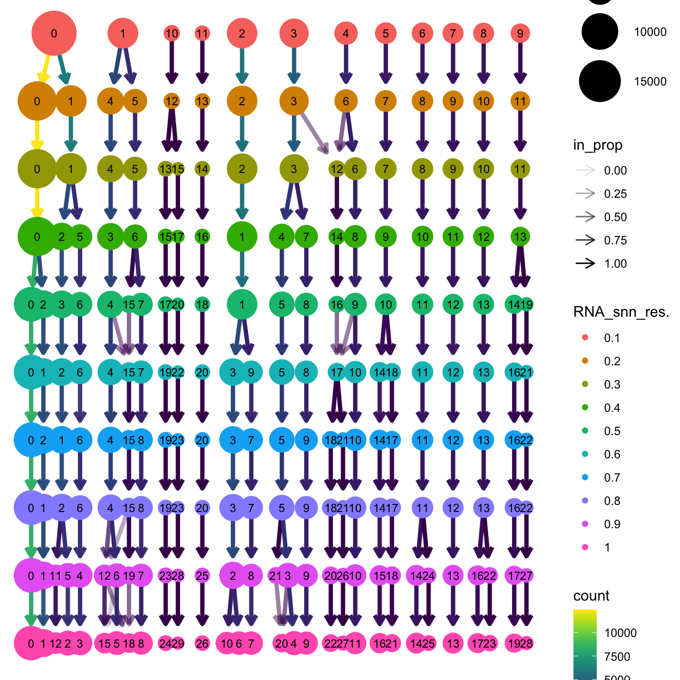

Past versions of clustree-1.png

Version	Author	Date
f460bd0	Gunjan Dixit	2024-04-26
9492583	Gunjan Dixit	2024-04-26

Based on the clustering tree, we chose an intermediate/optimum resolution where the clustering results are the most stable, with the least amount of shuffling cells.

opt_res <- "RNA_snn_res.0.4"  
n <- nlevels(seu_obj$RNA_snn_res.0.4)
seu_obj$RNA_snn_res.0.4 <- factor(seu_obj$RNA_snn_res.0.4, levels = seq(0,n-1))
seu_obj$seurat_clusters <- NULL
seu_obj$cluster <- seu_obj$RNA_snn_res.0.4
Idents(seu_obj) <- seu_obj$cluster

UMAP after clustering

Defining colours for each cell-type to be consistent with other age-related/cell type composition plots.

my_colors <- c(
  "B cells" = "steelblue",
  "CD4 T cells" = "brown",
  "Double negative T cells" = "gold",
  "CD8 T cells" = "lightgreen",
  "Pre B/T cells" = "orchid",
  "Innate lymphoid cells" = "tan",
  "Natural Killer cells" = "blueviolet",
  "Macrophages" = "green4",
  "Cycling T cells" = "turquoise",
  "Dendritic cells" = "grey80",
  "Gamma delta T cells" = "mediumvioletred",
  "Epithelial lineage" = "darkorange",
  "Granulocytes" = "olivedrab",
  "Fibroblast lineage" = "lavender",
  "None" = "white",
  "Monocytes" = "peachpuff",
  "Endothelial lineage" = "cadetblue",
  "SMG duct" = "lightpink",
  "Neuroendocrine" = "skyblue",
  "Doublet query/Other" = "#d62728"
)

UMAP displaying clusters at opt_res resolution and Broad cell Labels Level 3.

p1 <- DimPlot(seu_obj, reduction = "umap", raster = FALSE ,repel = TRUE, label = TRUE,label.size = 3.5, group.by = opt_res) +  NoLegend()

p2 <- DimPlot(seu_obj, reduction = "umap", raster = FALSE, repel = TRUE, label = TRUE, label.size = 3.5, group.by = "Broad_cell_label_3") + 
  scale_colour_manual(values = my_colors) + 
  ggtitle(paste0(tissue, ": UMAP (Azimuth Labels)")) 


p1 / p2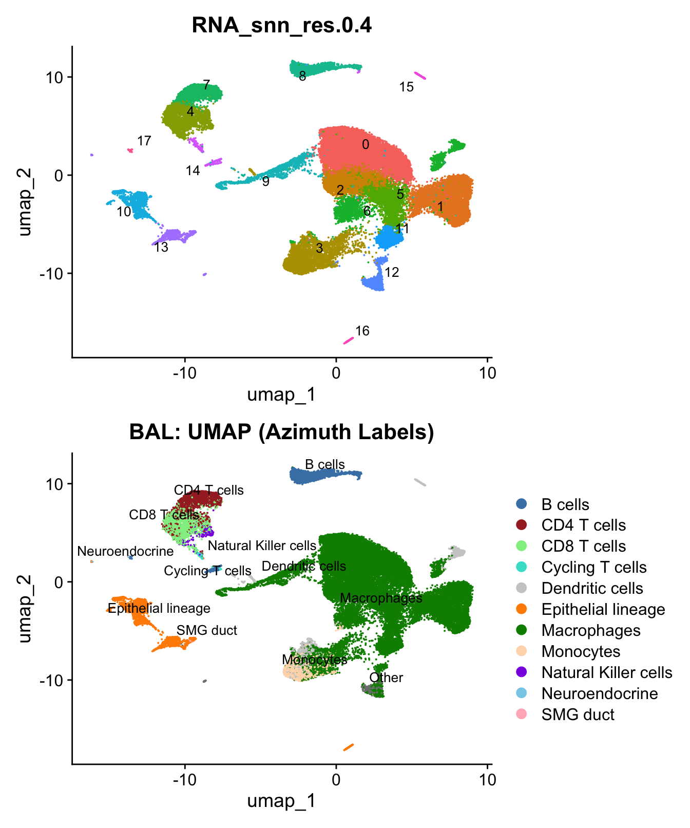 

Past versions of umap_after_clustering-1.png

Version	Author	Date
e0e83af	Gunjan Dixit	2024-06-04
320ccbd	Gunjan Dixit	2024-05-01
f460bd0	Gunjan Dixit	2024-04-26
9492583	Gunjan Dixit	2024-04-26

Save batch corrected Object

out1 <- here("output",
            "RDS", "AllBatches_Clustering_SEUs",
             paste0("G000231_Neeland_",tissue,".Clusters.SEU.rds"))
#dir.create(out1)
if (!file.exists(out1)) {
  saveRDS(seu_obj, file = out1)
}

Marker Gene Analysis

#seu_obj <- JoinLayers(seu_obj)
paed.markers <- FindAllMarkers(seu_obj, only.pos = TRUE, min.pct = 0.25, logfc.threshold = 0.25)

Extracting top 5 genes per cluster for visualization. The ‘top5’ contains the top 5 genes with the highest weighted average avg_log2FC within each cluster and the ‘best.wilcox.gene.per.cluster’ contains the single best gene with the highest weighted average avg_log2FC for each cluster.

paed.markers %>%
    group_by(cluster) %>% unique() %>% 
    top_n(n = 5, wt = avg_log2FC) -> top5

paed.markers %>%
    group_by(cluster) %>% 
    slice_head(n=1) %>% 
    pull(gene) -> best.wilcox.gene.per.cluster

best.wilcox.gene.per.cluster

 [1] "C8B"      "DEFB1"    "TMEM74B"  "SOCS3"    "CCL5"     "NR1H3"   
 [7] "VCAN"     "IL32"     "CD79A"    "TCF19"    "CTXN1"    "CXCL2"   
[13] "SLC11A1"  "KRT7"     "HIST1H1B" "PTPRS"    "KRT13"    "MZB1"    

Marker gene expression in clusters

This heatmap depicts the expression of top five genes in each cluster.

DoHeatmap(seu_obj, features = top5$gene) + NoLegend()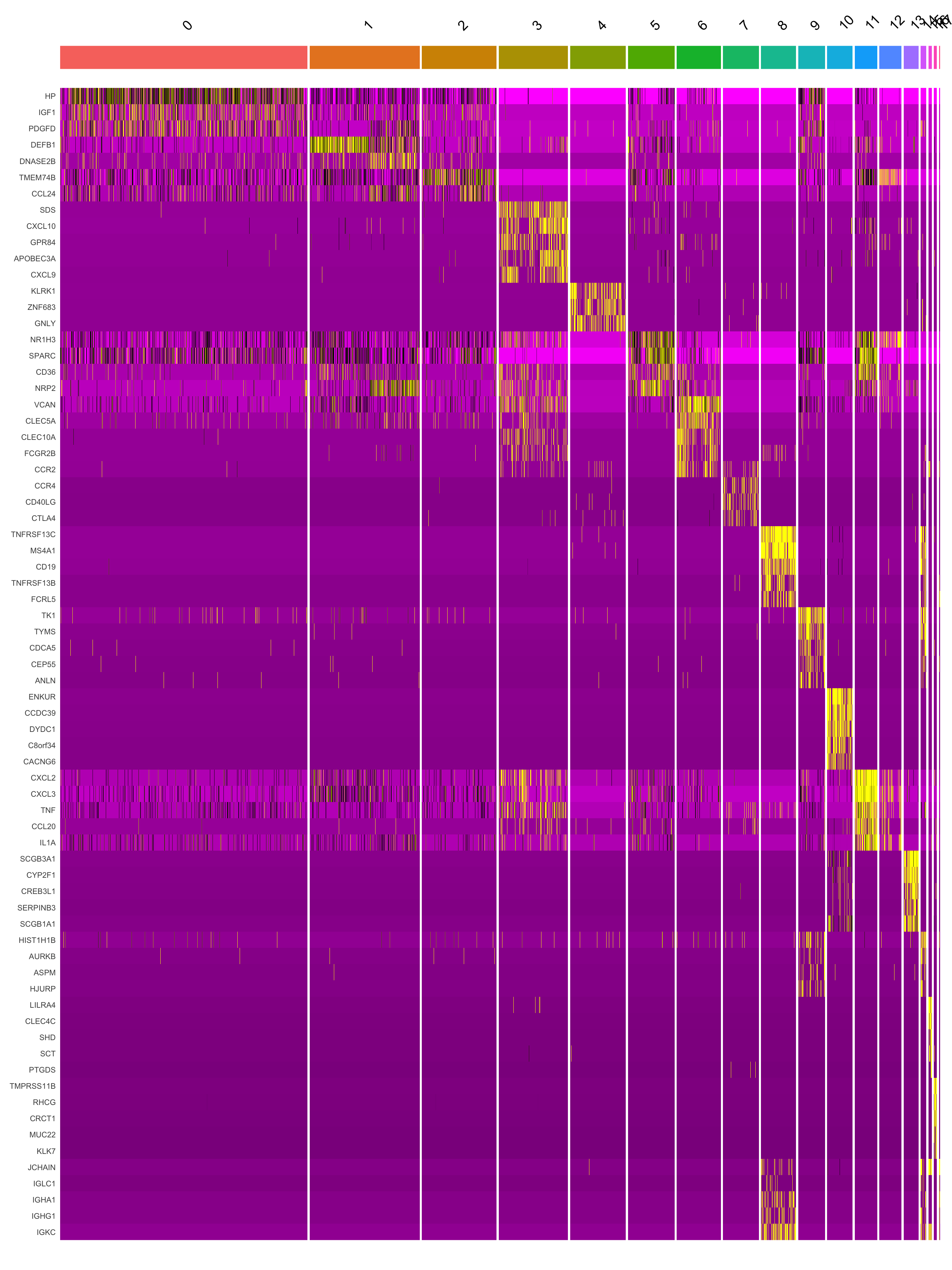

Past versions of top5_markers_heatmap-1.png

Version	Author	Date
320ccbd	Gunjan Dixit	2024-05-01

Violin plot shows the expression of top marker gene per cluster.

VlnPlot(seu_obj, features=best.wilcox.gene.per.cluster, ncol = 2, raster = FALSE, pt.size = FALSE)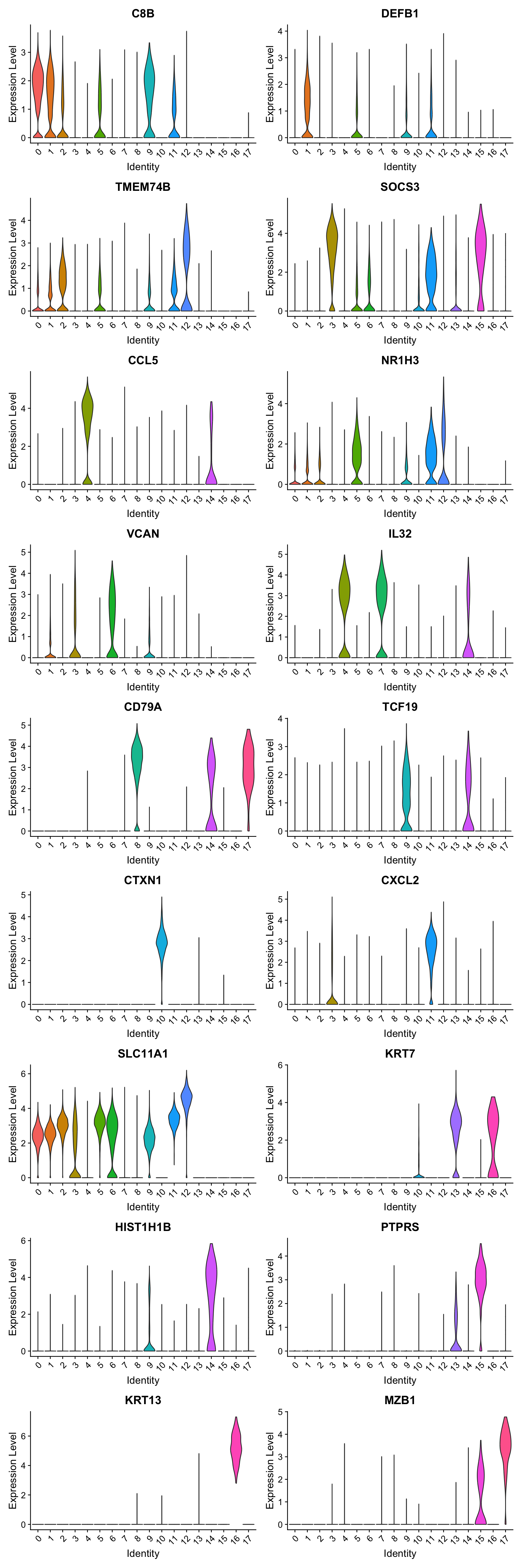

Past versions of top_marker_violinplot-1.png

Version	Author	Date
320ccbd	Gunjan Dixit	2024-05-01

Feature plot shows the expression of top marker genes per cluster.

FeaturePlot(seu_obj,features=best.wilcox.gene.per.cluster, reduction = 'umap', raster = FALSE, ncol = 2)

Past versions of top_marker_featureplot-1.png

Version	Author	Date
320ccbd	Gunjan Dixit	2024-05-01

Extract markers for each cluster

This section extracts marker genes for each cluster and save them as a CSV file.

out_markers <- here("output",
            "CSV", 
            paste(tissue,"_Marker_gene_clusters.",opt_res, sep = ""))

dir.create(out_markers, recursive = TRUE, showWarnings = FALSE)

for (cl in unique(paed.markers$cluster)) {
  cluster_data <- paed.markers %>% dplyr::filter(cluster == cl)
  file_name <- here(out_markers, paste0("G000231_Neeland_",tissue, "_cluster_", cl, ".csv"))
  write.csv(cluster_data, file = file_name)
}

Marker gene by limma-trend method (Jovana’s code)

#Idents(seu_obj) <- grp
seu_obj@meta.data$donor <- sub("_\\d+$", "", seu_obj@meta.data$Sample)

logcounts <- normCounts(DGEList(as.matrix(seu_obj[["RNA"]]$counts)),
                        log = TRUE, prior.count = 0.5)

Warning in asMethod(object): sparse->dense coercion: allocating vector of size
5.5 GiB

entrez <- AnnotationDbi::mapIds(org.Hs.eg.db,
                                keys = rownames(logcounts),
                                column = c("ENTREZID"),
                                keytype = "SYMBOL",
                                multiVals = "first")

'select()' returned 1:many mapping between keys and columns

logcounts <- logcounts[!is.na(entrez),]

maxclust <- length(levels(Idents(seu_obj))) - 1

clustgrp <- paste0("c", Idents(seu_obj))
clustgrp <- factor(clustgrp, levels = paste0("c", 0:maxclust))
sample <- seu_obj$donor

design <- model.matrix(~ 0 + clustgrp + sample)
colnames(design)[1:(length(levels(clustgrp)))] <- levels(clustgrp)

head(design)

  c0 c1 c2 c3 c4 c5 c6 c7 c8 c9 c10 c11 c12 c13 c14 c15 c16 c17 sampleeAIR035
1  0  0  0  0  0  0  0  0  0  0   0   0   0   0   0   0   1   0             0
2  0  1  0  0  0  0  0  0  0  0   0   0   0   0   0   0   0   0             0
3  0  0  0  0  0  0  0  1  0  0   0   0   0   0   0   0   0   0             0
4  0  1  0  0  0  0  0  0  0  0   0   0   0   0   0   0   0   0             0
5  0  1  0  0  0  0  0  0  0  0   0   0   0   0   0   0   0   0             0
6  0  1  0  0  0  0  0  0  0  0   0   0   0   0   0   0   0   0             0
  sampleeAIR036 sampleeAIR045 sampleeAIR046 sampleeAIR054 sampleeAIR057
1             0             0             0             0             0
2             0             0             0             0             0
3             0             0             0             0             0
4             0             0             0             0             0
5             0             0             0             0             0
6             0             0             0             0             0
  sampleeAIR059
1             0
2             0
3             0
4             0
5             0
6             0

# Create contrast matrix
mycont <- matrix(NA, ncol = length(levels(clustgrp)),
                 nrow = length(levels(clustgrp)))
rownames(mycont) <- colnames(mycont) <- levels(clustgrp)
diag(mycont) <- 1
mycont[upper.tri(mycont)] <- -1/(length(levels(factor(clustgrp))) - 1)
mycont[lower.tri(mycont)] <- -1/(length(levels(factor(clustgrp))) - 1)
mycont

             c0          c1          c2          c3          c4          c5
c0   1.00000000 -0.05882353 -0.05882353 -0.05882353 -0.05882353 -0.05882353
c1  -0.05882353  1.00000000 -0.05882353 -0.05882353 -0.05882353 -0.05882353
c2  -0.05882353 -0.05882353  1.00000000 -0.05882353 -0.05882353 -0.05882353
c3  -0.05882353 -0.05882353 -0.05882353  1.00000000 -0.05882353 -0.05882353
c4  -0.05882353 -0.05882353 -0.05882353 -0.05882353  1.00000000 -0.05882353
c5  -0.05882353 -0.05882353 -0.05882353 -0.05882353 -0.05882353  1.00000000
c6  -0.05882353 -0.05882353 -0.05882353 -0.05882353 -0.05882353 -0.05882353
c7  -0.05882353 -0.05882353 -0.05882353 -0.05882353 -0.05882353 -0.05882353
c8  -0.05882353 -0.05882353 -0.05882353 -0.05882353 -0.05882353 -0.05882353
c9  -0.05882353 -0.05882353 -0.05882353 -0.05882353 -0.05882353 -0.05882353
c10 -0.05882353 -0.05882353 -0.05882353 -0.05882353 -0.05882353 -0.05882353
c11 -0.05882353 -0.05882353 -0.05882353 -0.05882353 -0.05882353 -0.05882353
c12 -0.05882353 -0.05882353 -0.05882353 -0.05882353 -0.05882353 -0.05882353
c13 -0.05882353 -0.05882353 -0.05882353 -0.05882353 -0.05882353 -0.05882353
c14 -0.05882353 -0.05882353 -0.05882353 -0.05882353 -0.05882353 -0.05882353
c15 -0.05882353 -0.05882353 -0.05882353 -0.05882353 -0.05882353 -0.05882353
c16 -0.05882353 -0.05882353 -0.05882353 -0.05882353 -0.05882353 -0.05882353
c17 -0.05882353 -0.05882353 -0.05882353 -0.05882353 -0.05882353 -0.05882353
             c6          c7          c8          c9         c10         c11
c0  -0.05882353 -0.05882353 -0.05882353 -0.05882353 -0.05882353 -0.05882353
c1  -0.05882353 -0.05882353 -0.05882353 -0.05882353 -0.05882353 -0.05882353
c2  -0.05882353 -0.05882353 -0.05882353 -0.05882353 -0.05882353 -0.05882353
c3  -0.05882353 -0.05882353 -0.05882353 -0.05882353 -0.05882353 -0.05882353
c4  -0.05882353 -0.05882353 -0.05882353 -0.05882353 -0.05882353 -0.05882353
c5  -0.05882353 -0.05882353 -0.05882353 -0.05882353 -0.05882353 -0.05882353
c6   1.00000000 -0.05882353 -0.05882353 -0.05882353 -0.05882353 -0.05882353
c7  -0.05882353  1.00000000 -0.05882353 -0.05882353 -0.05882353 -0.05882353
c8  -0.05882353 -0.05882353  1.00000000 -0.05882353 -0.05882353 -0.05882353
c9  -0.05882353 -0.05882353 -0.05882353  1.00000000 -0.05882353 -0.05882353
c10 -0.05882353 -0.05882353 -0.05882353 -0.05882353  1.00000000 -0.05882353
c11 -0.05882353 -0.05882353 -0.05882353 -0.05882353 -0.05882353  1.00000000
c12 -0.05882353 -0.05882353 -0.05882353 -0.05882353 -0.05882353 -0.05882353
c13 -0.05882353 -0.05882353 -0.05882353 -0.05882353 -0.05882353 -0.05882353
c14 -0.05882353 -0.05882353 -0.05882353 -0.05882353 -0.05882353 -0.05882353
c15 -0.05882353 -0.05882353 -0.05882353 -0.05882353 -0.05882353 -0.05882353
c16 -0.05882353 -0.05882353 -0.05882353 -0.05882353 -0.05882353 -0.05882353
c17 -0.05882353 -0.05882353 -0.05882353 -0.05882353 -0.05882353 -0.05882353
            c12         c13         c14         c15         c16         c17
c0  -0.05882353 -0.05882353 -0.05882353 -0.05882353 -0.05882353 -0.05882353
c1  -0.05882353 -0.05882353 -0.05882353 -0.05882353 -0.05882353 -0.05882353
c2  -0.05882353 -0.05882353 -0.05882353 -0.05882353 -0.05882353 -0.05882353
c3  -0.05882353 -0.05882353 -0.05882353 -0.05882353 -0.05882353 -0.05882353
c4  -0.05882353 -0.05882353 -0.05882353 -0.05882353 -0.05882353 -0.05882353
c5  -0.05882353 -0.05882353 -0.05882353 -0.05882353 -0.05882353 -0.05882353
c6  -0.05882353 -0.05882353 -0.05882353 -0.05882353 -0.05882353 -0.05882353
c7  -0.05882353 -0.05882353 -0.05882353 -0.05882353 -0.05882353 -0.05882353
c8  -0.05882353 -0.05882353 -0.05882353 -0.05882353 -0.05882353 -0.05882353
c9  -0.05882353 -0.05882353 -0.05882353 -0.05882353 -0.05882353 -0.05882353
c10 -0.05882353 -0.05882353 -0.05882353 -0.05882353 -0.05882353 -0.05882353
c11 -0.05882353 -0.05882353 -0.05882353 -0.05882353 -0.05882353 -0.05882353
c12  1.00000000 -0.05882353 -0.05882353 -0.05882353 -0.05882353 -0.05882353
c13 -0.05882353  1.00000000 -0.05882353 -0.05882353 -0.05882353 -0.05882353
c14 -0.05882353 -0.05882353  1.00000000 -0.05882353 -0.05882353 -0.05882353
c15 -0.05882353 -0.05882353 -0.05882353  1.00000000 -0.05882353 -0.05882353
c16 -0.05882353 -0.05882353 -0.05882353 -0.05882353  1.00000000 -0.05882353
c17 -0.05882353 -0.05882353 -0.05882353 -0.05882353 -0.05882353  1.00000000

# Fill out remaining rows with 0s
zero.rows <- matrix(0, ncol = length(levels(clustgrp)),
                    nrow = (ncol(design) - length(levels(clustgrp))))
fullcont <- rbind(mycont, zero.rows)
rownames(fullcont) <- colnames(design)

fit <- lmFit(logcounts, design)

fit.cont <- contrasts.fit(fit, contrasts = fullcont)
fit.cont <- eBayes(fit.cont, trend = TRUE, robust = TRUE)

Warning: 519 very small variances detected, have been offset away from zero

summary(decideTests(fit.cont))

          c0    c1    c2    c3    c4    c5    c6    c7    c8    c9   c10   c11
Down    6696  5799  5113 10187  9743  4752  5740  9122  8810  4551  4055  4469
NotSig  5370  5844  6055  4795  5145  6962  7313  5814  5791  6576  5171  9110
Up      5045  5468  5943  2129  2223  5397  4058  2175  2510  5984  7885  3532
         c12   c13   c14   c15   c16   c17
Down    8152  4497  4023  3989  8068  4040
NotSig  6085  7580  8833 11289  7254 12425
Up      2874  5034  4255  1833  1789   646

Test relative to a threshold (TREAT)

tr <- treat(fit.cont, lfc = 0.5)
dt <- decideTests(tr)
summary(dt)

          c0    c1    c2    c3    c4    c5    c6    c7    c8    c9   c10   c11
Down      53    44    62   121   536    48    33   497   491    39   426    53
NotSig 16422 16337 16450 16616 16375 16523 16759 16401 16342 16464 15248 16561
Up       636   730   599   374   200   540   319   213   278   608  1437   497
         c12   c13   c14   c15   c16   c17
Down     482   400   303   226   610   362
NotSig 16401 16252 16349 16565 15993 16640
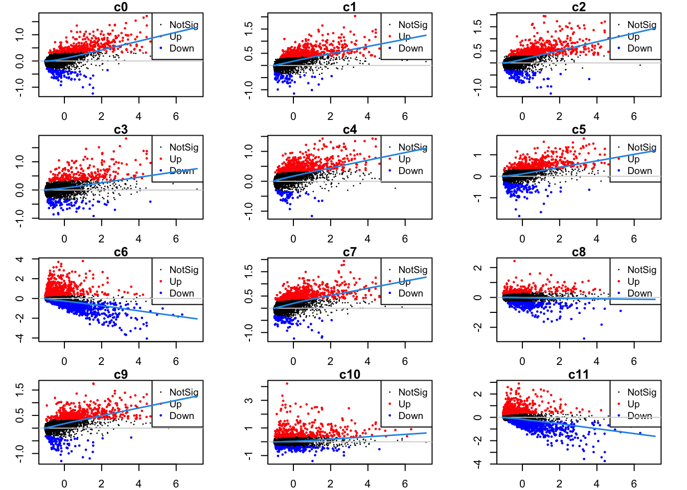
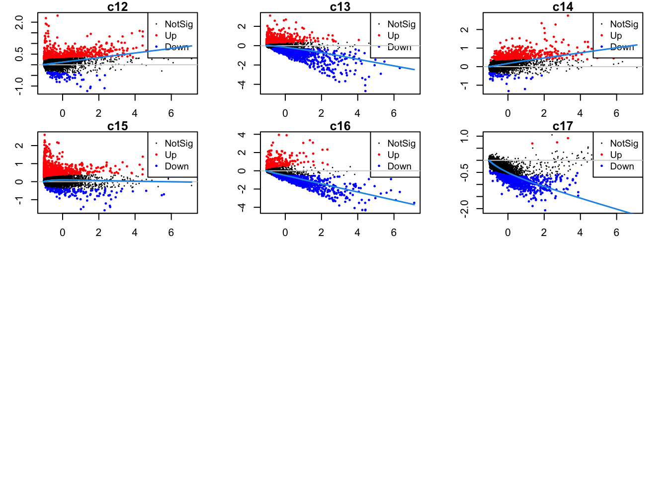
Up       228   459   459   320   508   109

Mean-difference plots per cluster

par(mfrow=c(4,3))
par(mar=c(2,3,1,2))

for(i in 1:ncol(mycont)){
  plotMD(tr, coef = i, status = dt[,i], hl.cex = 0.5)
  abline(h = 0, col = "lightgrey")
  lines(lowess(tr$Amean, tr$coefficients[,i]), lwd = 1.5, col = 4)
}

Past versions of unnamed-chunk-5-1.png

Version	Author	Date
75b471c	Gunjan Dixit	2024-06-28
324c175	Gunjan Dixit	2024-06-28
e0e83af	Gunjan Dixit	2024-06-04
f460bd0	Gunjan Dixit	2024-04-26
9492583	Gunjan Dixit	2024-04-26

Past versions of unnamed-chunk-5-2.png

Version	Author	Date
75b471c	Gunjan Dixit	2024-06-28
324c175	Gunjan Dixit	2024-06-28
e0e83af	Gunjan Dixit	2024-06-04

Reactome pathways using CameraPR

if(!file.exists(here("data/Hs.c2.cp.reactome.v7.1.entrez.rds")))
  download.file("https://bioinf.wehi.edu.au/MSigDB/v7.1/Hs.c2.cp.reactome.v7.1.entrez.rds",
                here("data/Hs.c2.cp.reactome.v7.1.entrez.rds"))
Hs.c2.reactome <- readRDS(here("data/Hs.c2.cp.reactome.v7.1.entrez.rds"))

gns <- AnnotationDbi::mapIds(org.Hs.eg.db, 
                             keys = rownames(tr), 
                             column = c("ENTREZID"),
                             keytype = "SYMBOL",
                             multiVals = "first")

'select()' returned 1:many mapping between keys and columns

options(scipen=-1, digits = 6)
contnames <- colnames(mycont)

out_markers1 <- here("output",
            "CSV", 
            paste(tissue,"_Marker_gene_clusters.limmaTrend",opt_res, sep = ""))

dir.create(out_markers1, recursive = TRUE, showWarnings = FALSE)

for(i in levels(paed.markers$cluster)){
  top <- paed.markers[paed.markers$cluster == i,]
  
  write.csv(top, file = glue("{out_markers1}/up-cluster-seurat-c{i}.csv"))
  
  top <- topTreat(tr, coef = glue("c{i}"), n = Inf)
  top <- top[top$logFC > 0, ]

  write.csv(top[1:100, ],
            file = glue("{out_markers1}/up-cluster-limma-c{i}.csv"))

  # gene set testing results
  c2.id <- ids2indices(Hs.c2.reactome, unname(gns[rownames(tr)]))

  cameraPR(tr$t[,glue("c{i}")], c2.id) %>%
    rownames_to_column(var = "Pathway") %>%
    slice_head(n = 50) %>%
    write_csv(file = here(glue("{out_markers1}/REACTOME-cluster-limma-c{i}.csv")))
}

files <- file.path(here("output/CSV/BAL_Marker_gene_clusters.limmaTrendRNA_snn_res.0.4/"), 
                   sprintf("REACTOME-cluster-limma-c%s.csv", 0:17))

for (file in files) {
   data <- read_csv(file) %>%
    arrange(PValue) %>%  
    slice_head(n = 30)   

  cluster <- gsub(".*limma-c(\\d+)\\.csv", "Cluster \\1", basename(file))

  p <- ggplot(data, aes(x = reorder(Pathway, -log10(PValue)), y = -log10(PValue), size = NGenes, color = Direction)) +
    geom_point(alpha = 0.7) +
    coord_flip() +
    scale_color_manual(values = c(Up = "green3", Down = "red3")) + 
    labs(title = cluster, x = NULL, y = "-log10(P-value)", size = "Number of Genes", color = "Direction") +
    theme_minimal() +
    theme(axis.text.y = element_text(size = 8), plot.title = element_text(hjust = 0.5))
  
  print(p)
}

Past versions of unnamed-chunk-8-1.png

Version	Author	Date
75b471c	Gunjan Dixit	2024-06-28
324c175	Gunjan Dixit	2024-06-28
e0e83af	Gunjan Dixit	2024-06-04

Past versions of unnamed-chunk-8-2.png

Version	Author	Date
75b471c	Gunjan Dixit	2024-06-28
324c175	Gunjan Dixit	2024-06-28
e0e83af	Gunjan Dixit	2024-06-04

Past versions of unnamed-chunk-8-3.png

Version	Author	Date
75b471c	Gunjan Dixit	2024-06-28
324c175	Gunjan Dixit	2024-06-28
e0e83af	Gunjan Dixit	2024-06-04

Past versions of unnamed-chunk-8-4.png

Version	Author	Date
75b471c	Gunjan Dixit	2024-06-28
324c175	Gunjan Dixit	2024-06-28
e0e83af	Gunjan Dixit	2024-06-04

Past versions of unnamed-chunk-8-5.png

Version	Author	Date
75b471c	Gunjan Dixit	2024-06-28
324c175	Gunjan Dixit	2024-06-28
e0e83af	Gunjan Dixit	2024-06-04

Past versions of unnamed-chunk-8-6.png

Version	Author	Date
75b471c	Gunjan Dixit	2024-06-28
324c175	Gunjan Dixit	2024-06-28
e0e83af	Gunjan Dixit	2024-06-04

Past versions of unnamed-chunk-8-7.png

Version	Author	Date
75b471c	Gunjan Dixit	2024-06-28
324c175	Gunjan Dixit	2024-06-28
e0e83af	Gunjan Dixit	2024-06-04

Past versions of unnamed-chunk-8-8.png

Version	Author	Date
75b471c	Gunjan Dixit	2024-06-28
324c175	Gunjan Dixit	2024-06-28
e0e83af	Gunjan Dixit	2024-06-04

Past versions of unnamed-chunk-8-9.png

Version	Author	Date
75b471c	Gunjan Dixit	2024-06-28
324c175	Gunjan Dixit	2024-06-28
e0e83af	Gunjan Dixit	2024-06-04

Past versions of unnamed-chunk-8-10.png

Version	Author	Date
75b471c	Gunjan Dixit	2024-06-28
324c175	Gunjan Dixit	2024-06-28
e0e83af	Gunjan Dixit	2024-06-04

Past versions of unnamed-chunk-8-11.png

Version	Author	Date
75b471c	Gunjan Dixit	2024-06-28
324c175	Gunjan Dixit	2024-06-28
e0e83af	Gunjan Dixit	2024-06-04

Past versions of unnamed-chunk-8-12.png

Version	Author	Date
75b471c	Gunjan Dixit	2024-06-28
324c175	Gunjan Dixit	2024-06-28
e0e83af	Gunjan Dixit	2024-06-04

Past versions of unnamed-chunk-8-13.png

Version	Author	Date
75b471c	Gunjan Dixit	2024-06-28
324c175	Gunjan Dixit	2024-06-28
e0e83af	Gunjan Dixit	2024-06-04

Past versions of unnamed-chunk-8-14.png

Version	Author	Date
75b471c	Gunjan Dixit	2024-06-28
324c175	Gunjan Dixit	2024-06-28
e0e83af	Gunjan Dixit	2024-06-04

Past versions of unnamed-chunk-8-15.png

Version	Author	Date
75b471c	Gunjan Dixit	2024-06-28
324c175	Gunjan Dixit	2024-06-28
e0e83af	Gunjan Dixit	2024-06-04

Past versions of unnamed-chunk-8-16.png

Version	Author	Date
75b471c	Gunjan Dixit	2024-06-28
324c175	Gunjan Dixit	2024-06-28
e0e83af	Gunjan Dixit	2024-06-04

Past versions of unnamed-chunk-8-17.png

Version	Author	Date
75b471c	Gunjan Dixit	2024-06-28
324c175	Gunjan Dixit	2024-06-28
e0e83af	Gunjan Dixit	2024-06-04

Past versions of unnamed-chunk-8-18.png

Version	Author	Date
75b471c	Gunjan Dixit	2024-06-28
324c175	Gunjan Dixit	2024-06-28
e0e83af	Gunjan Dixit	2024-06-04

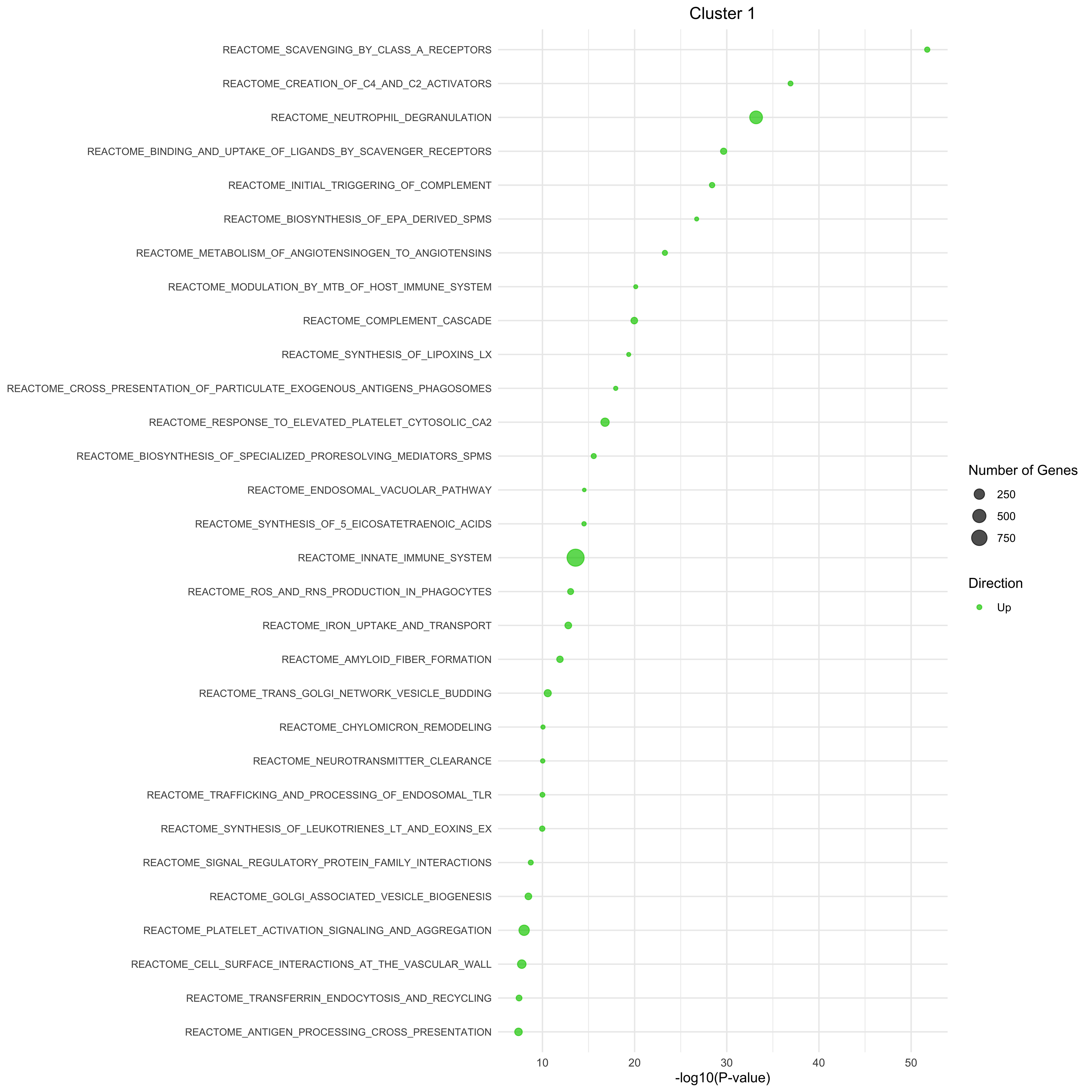
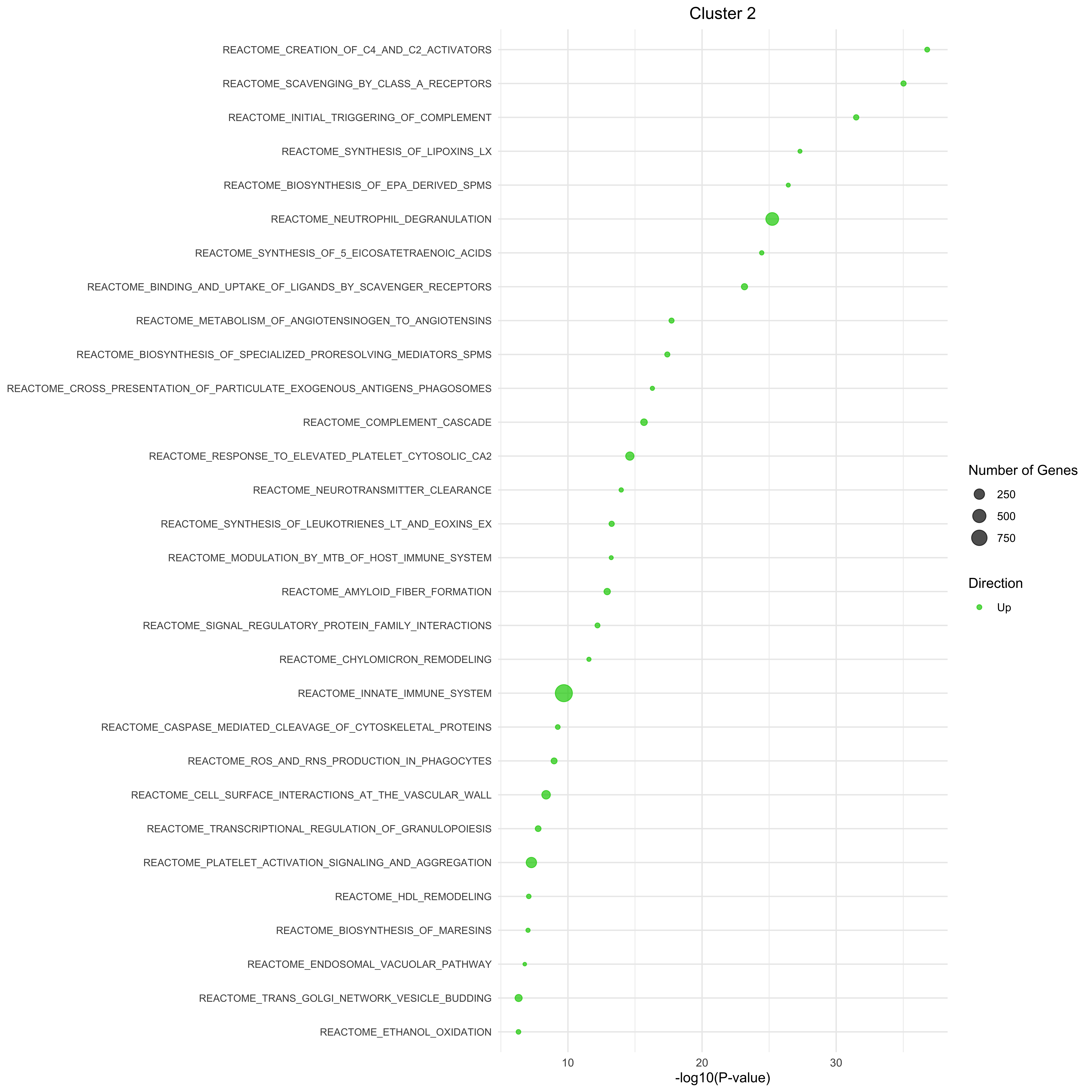
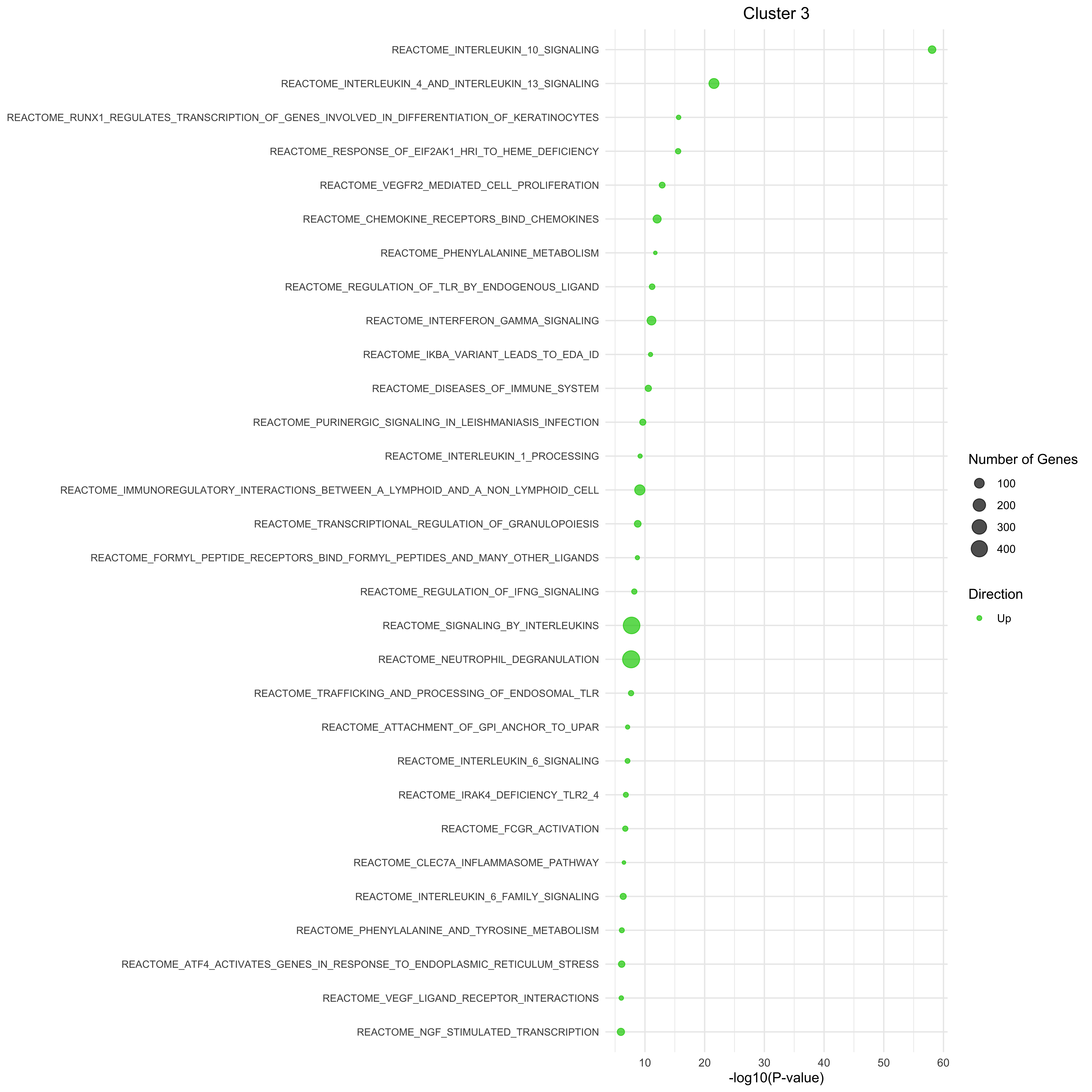
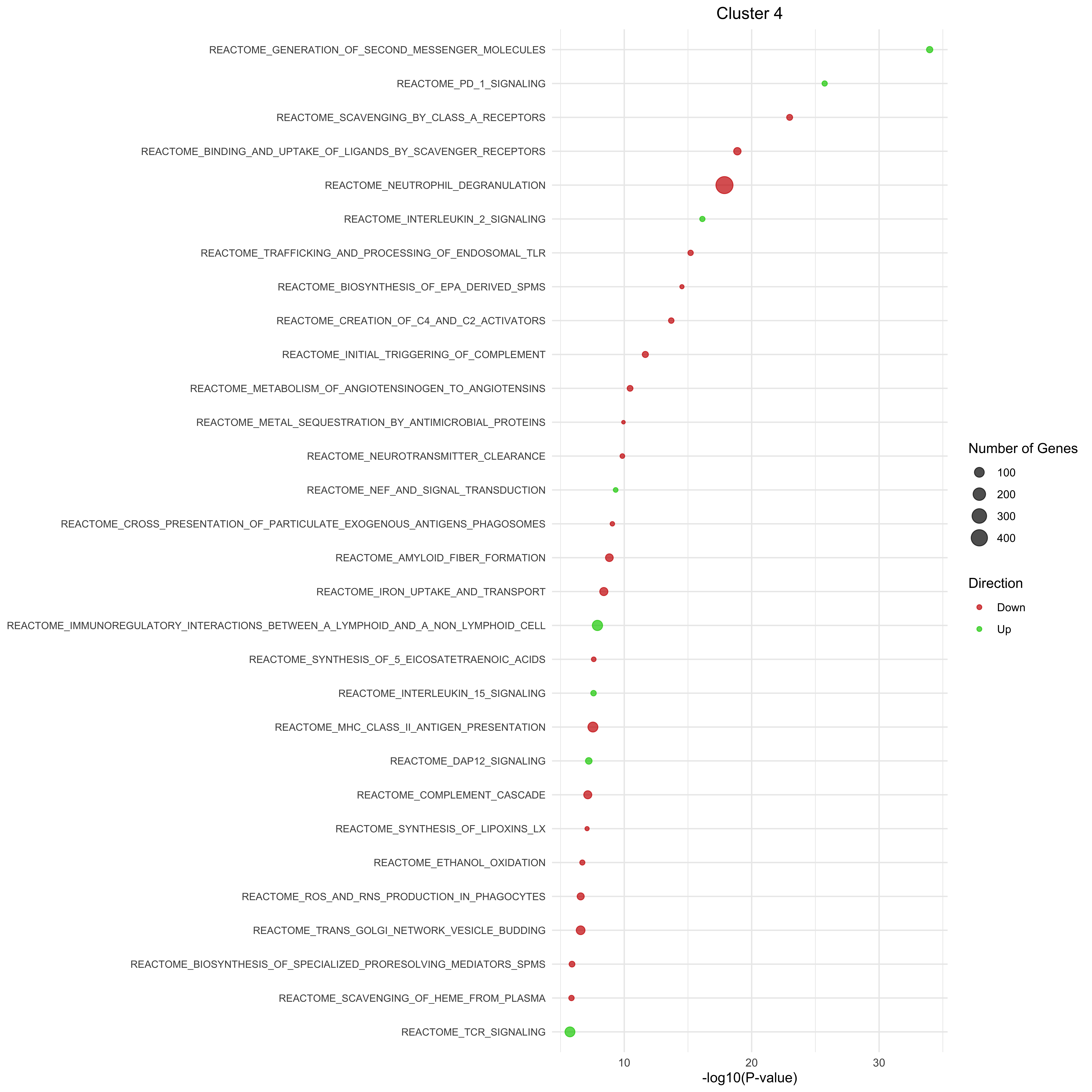
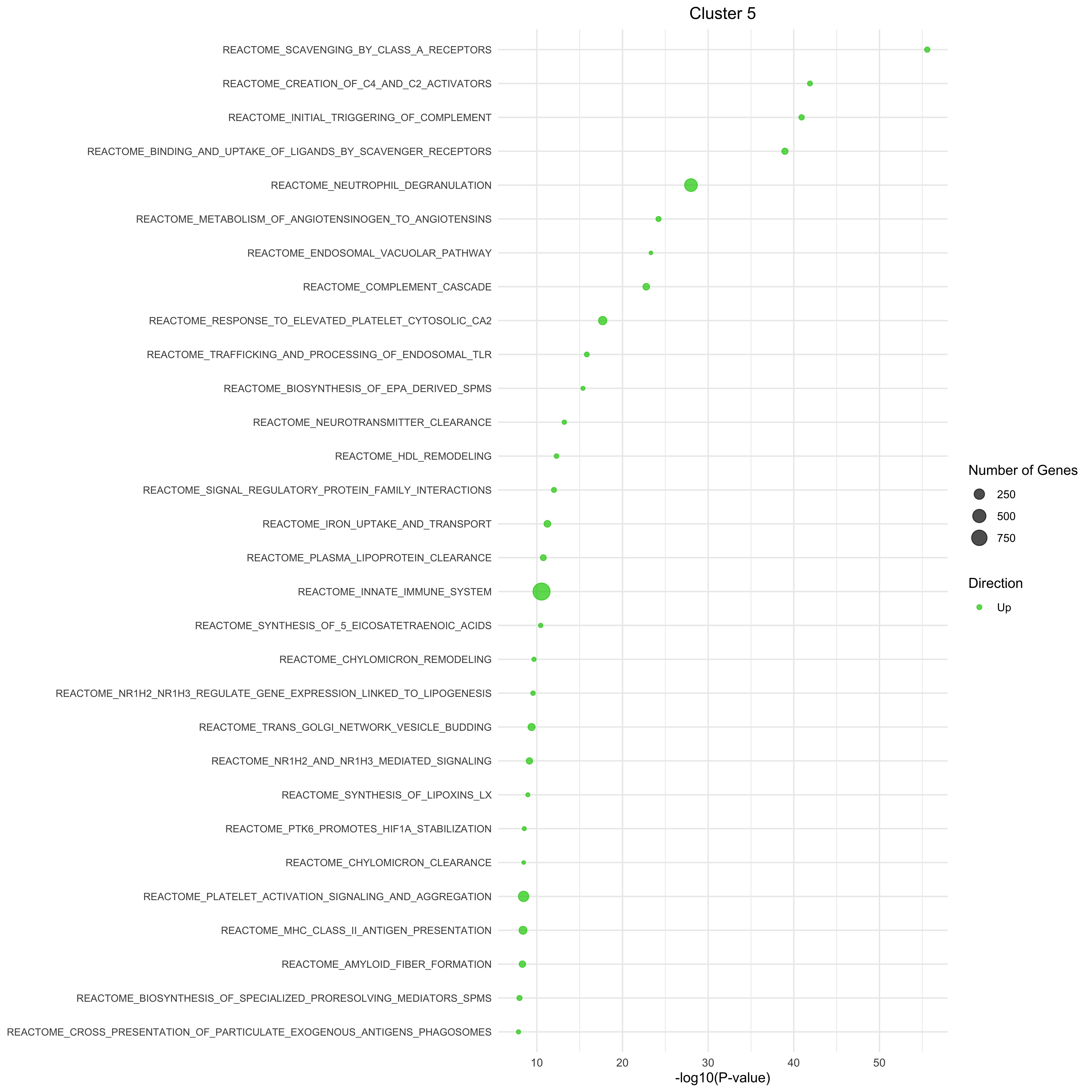
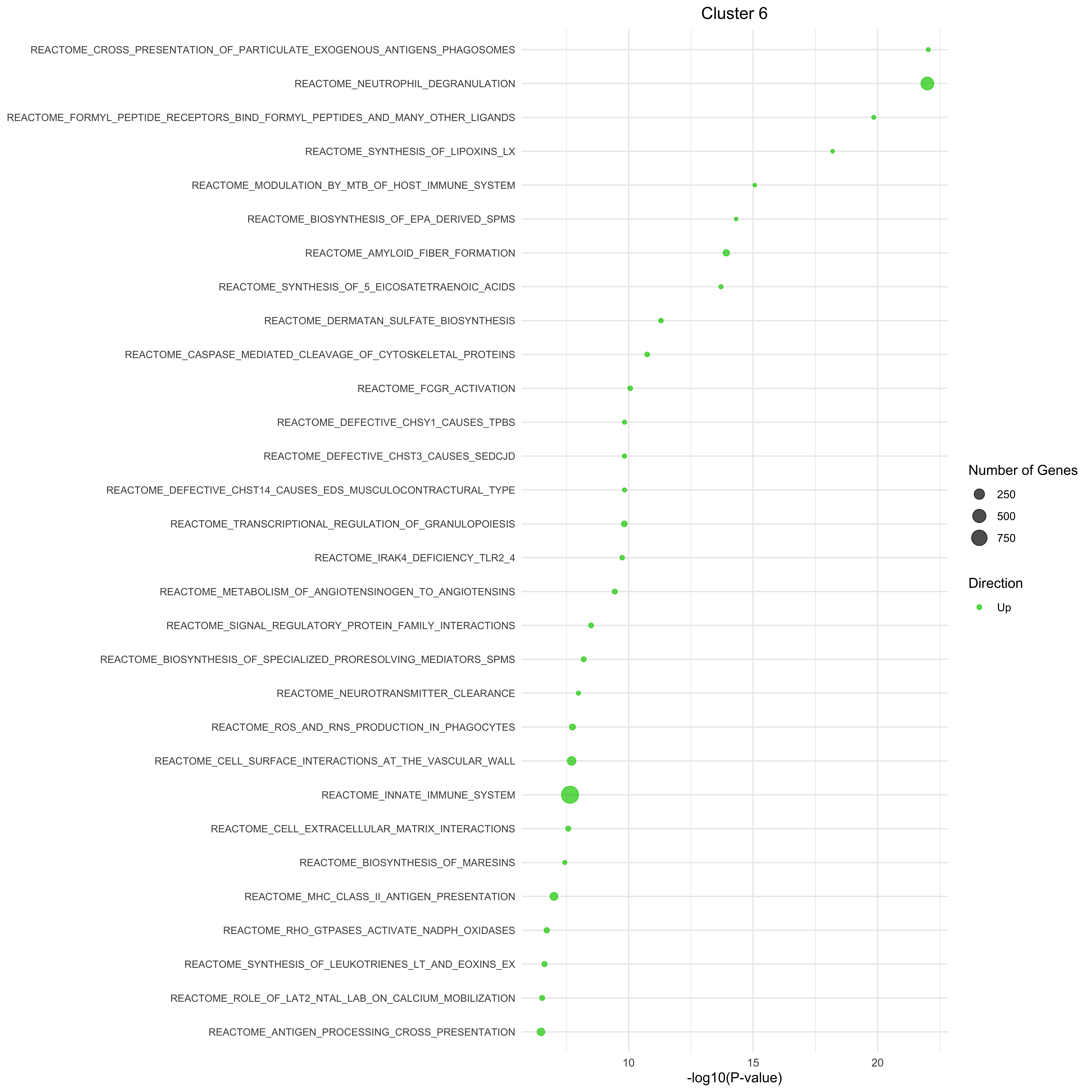
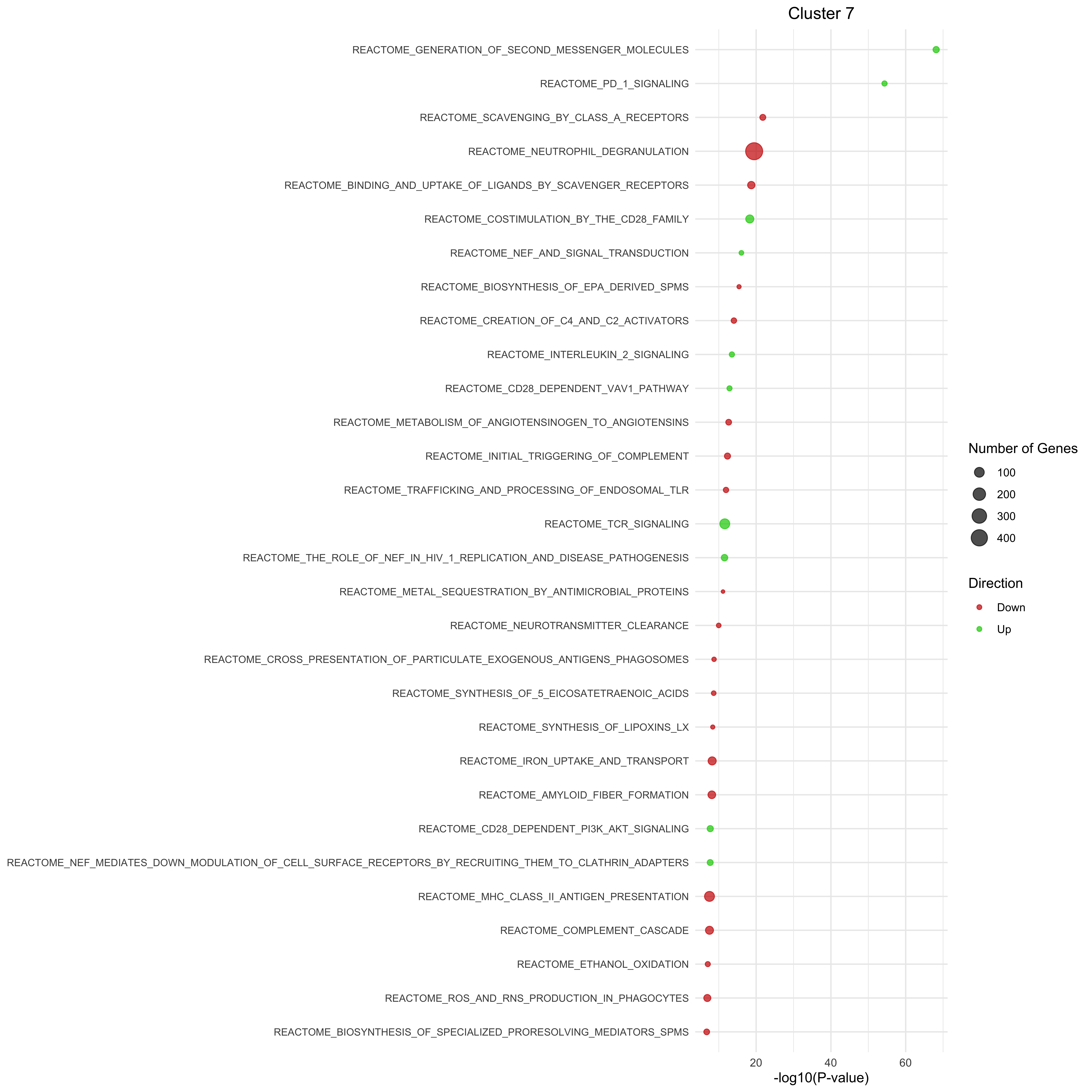
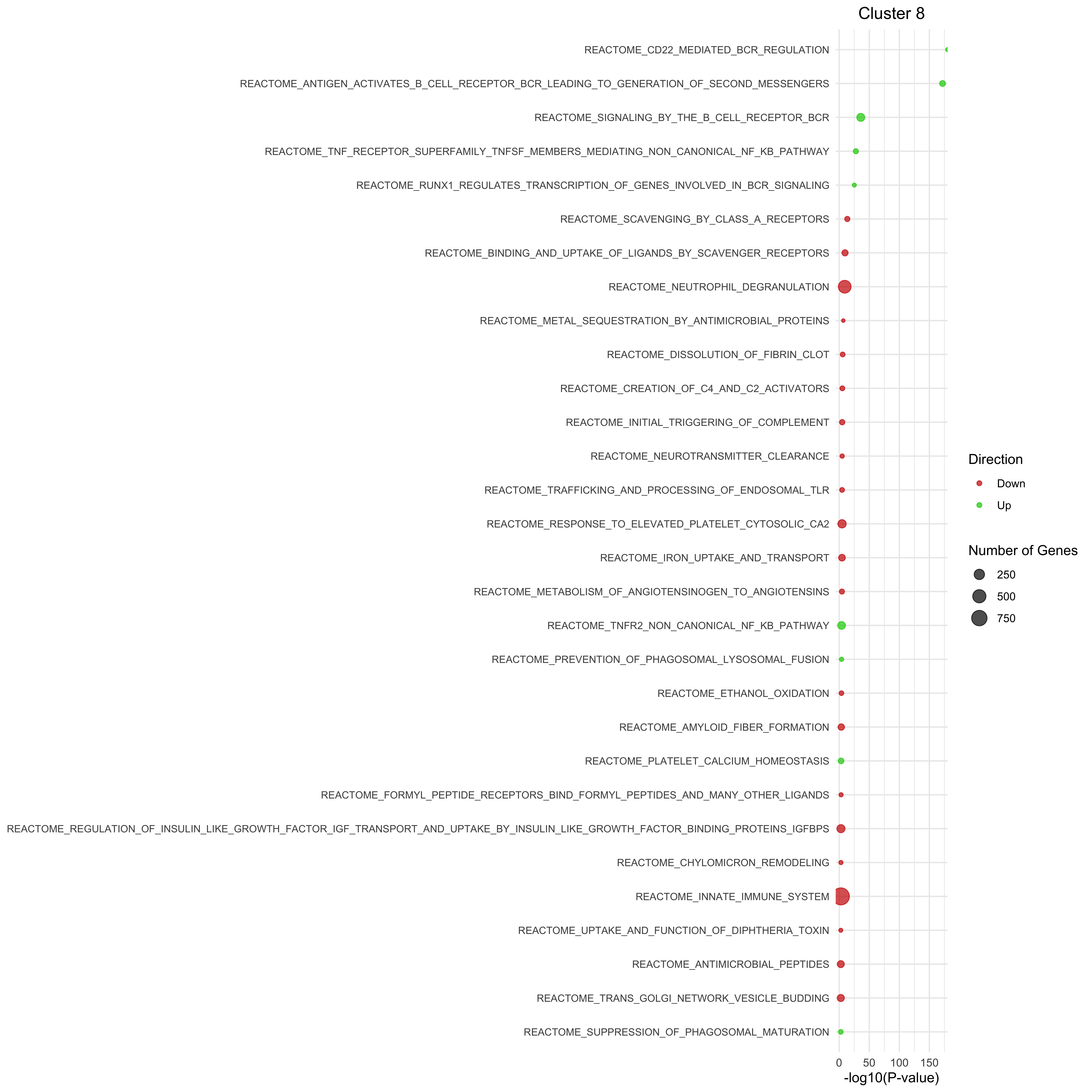
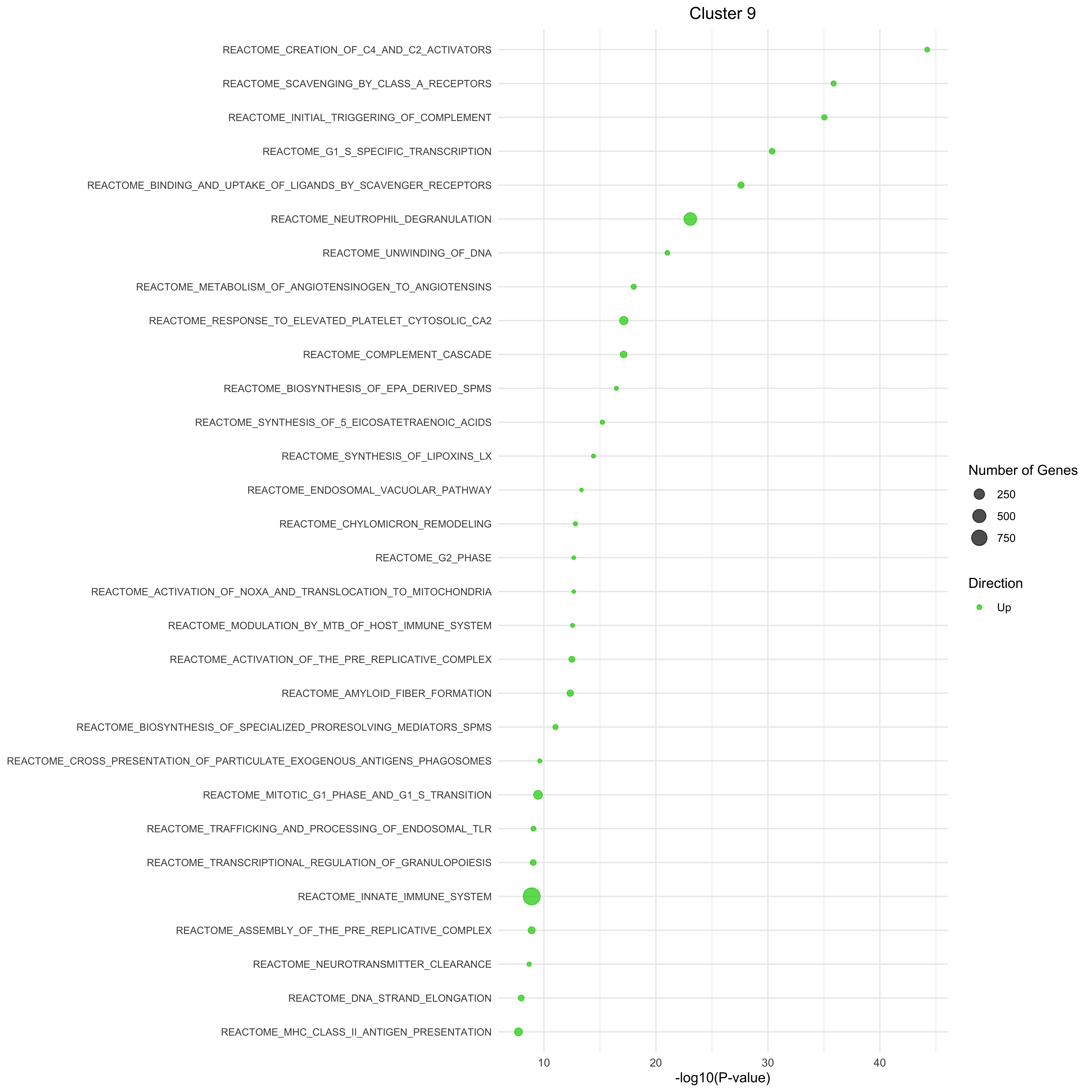
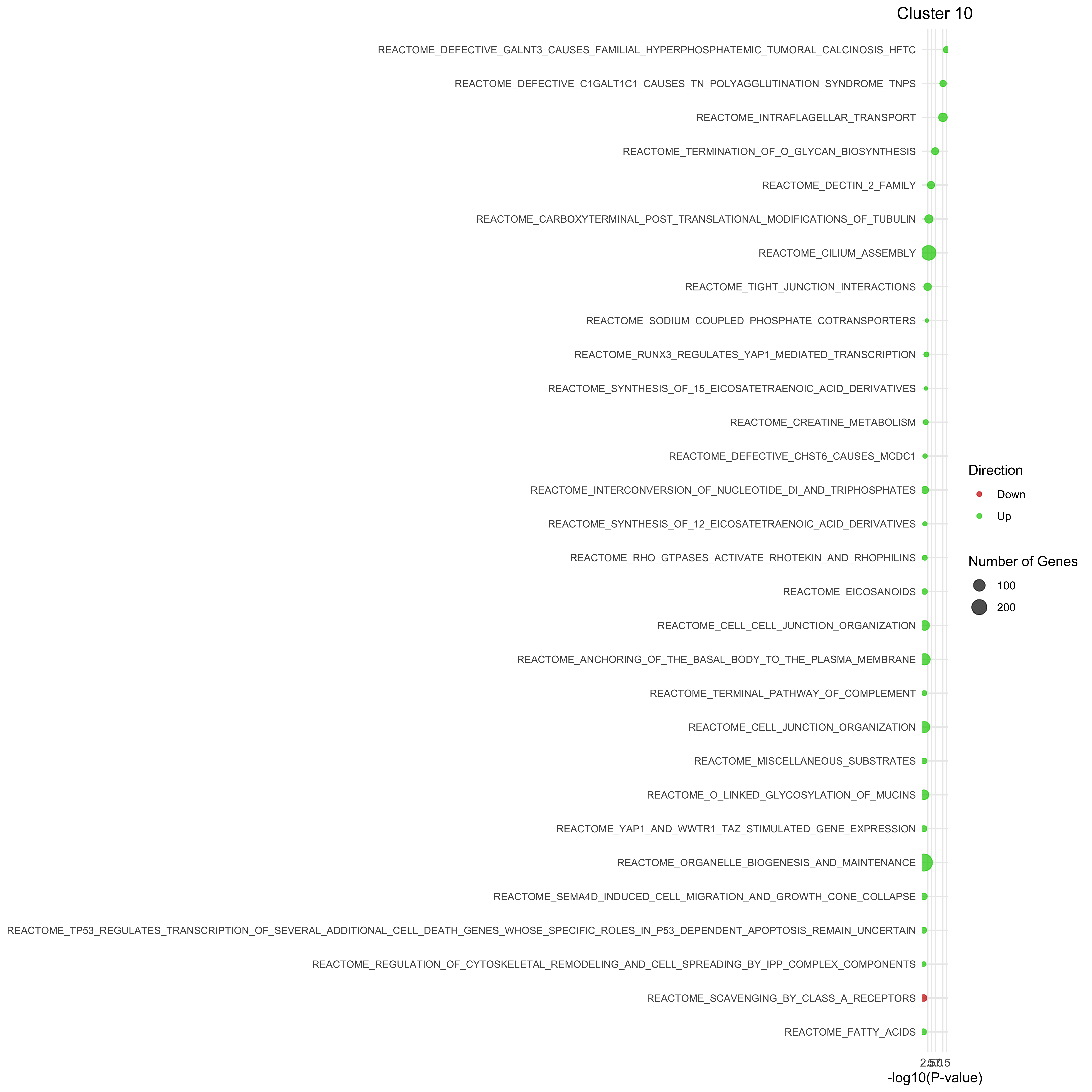
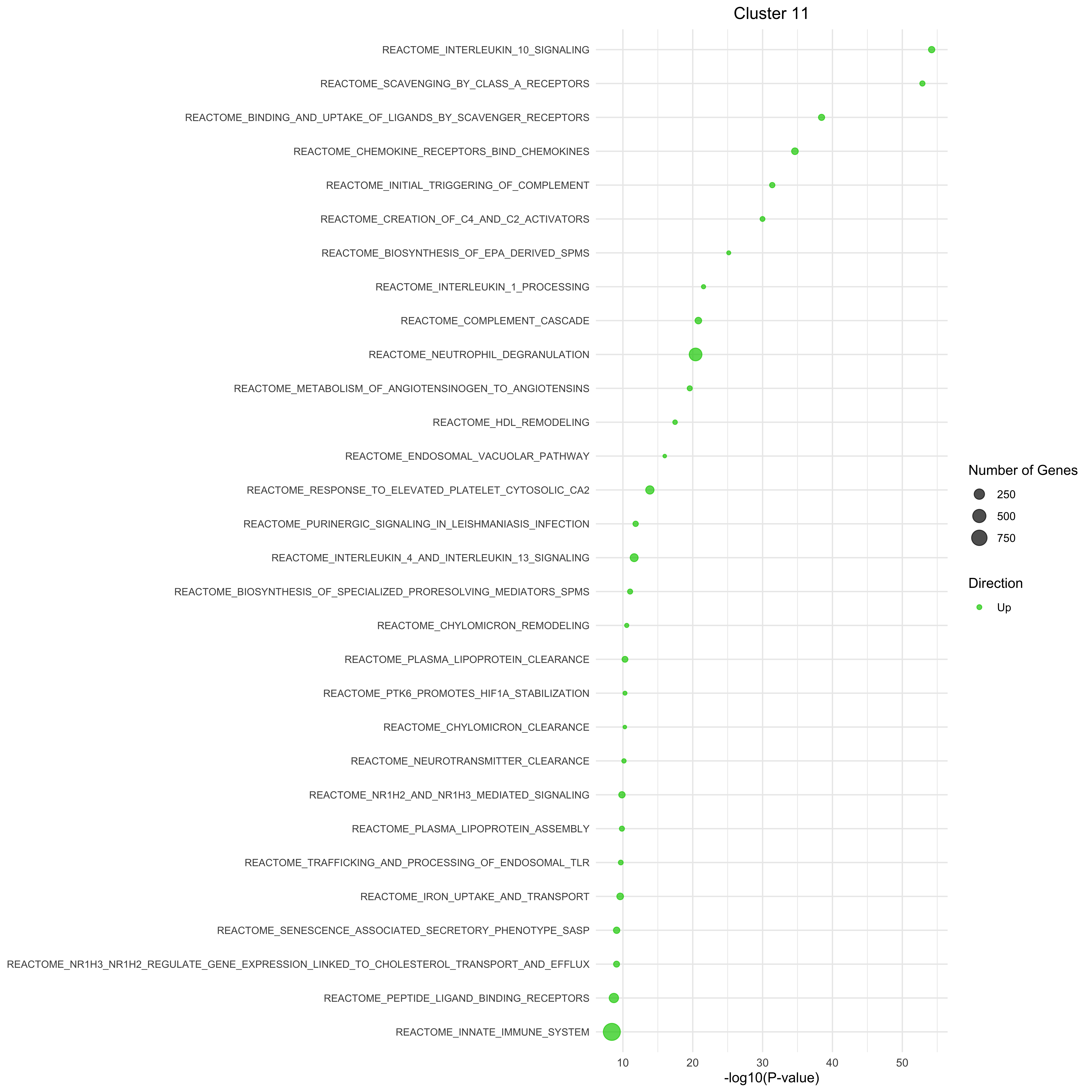
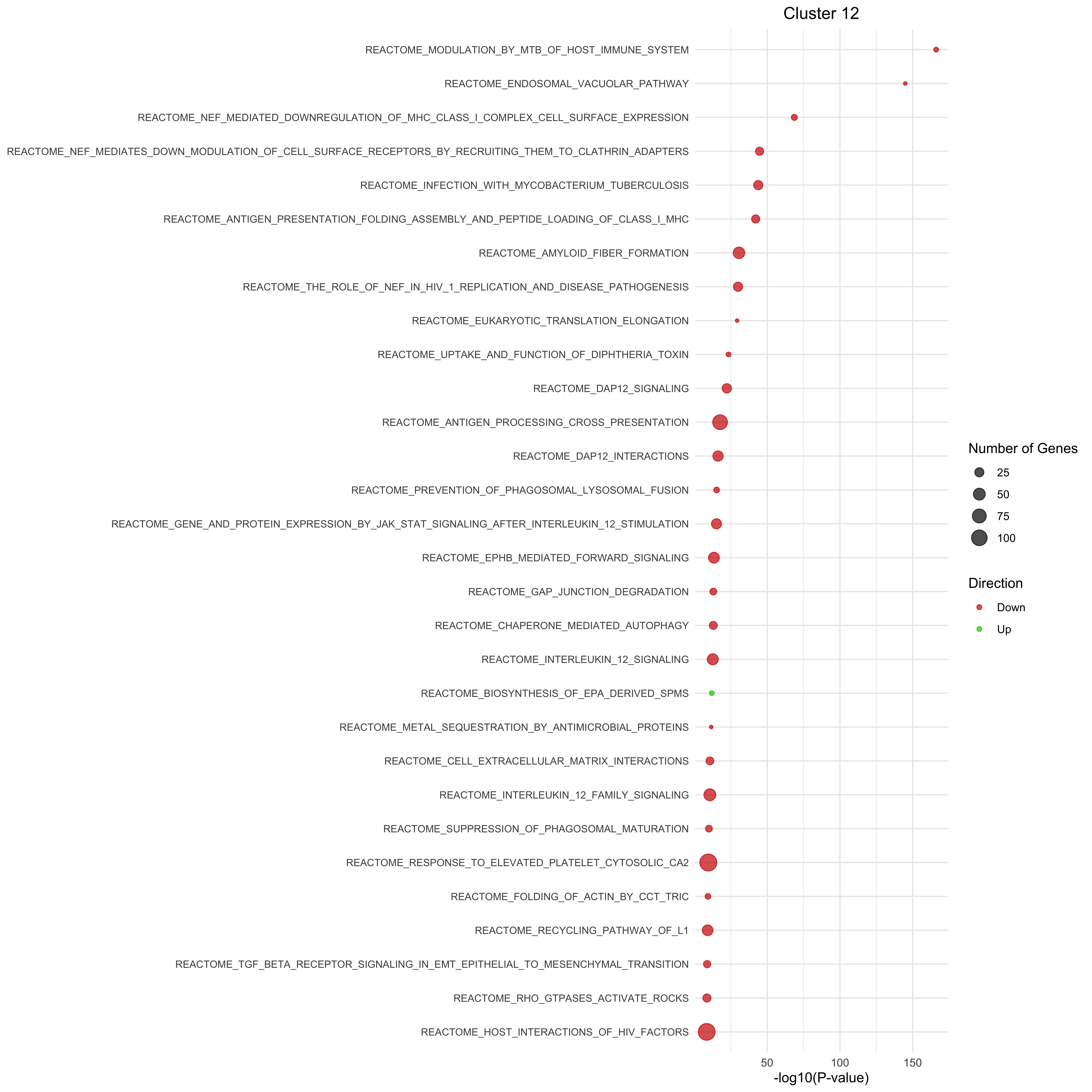
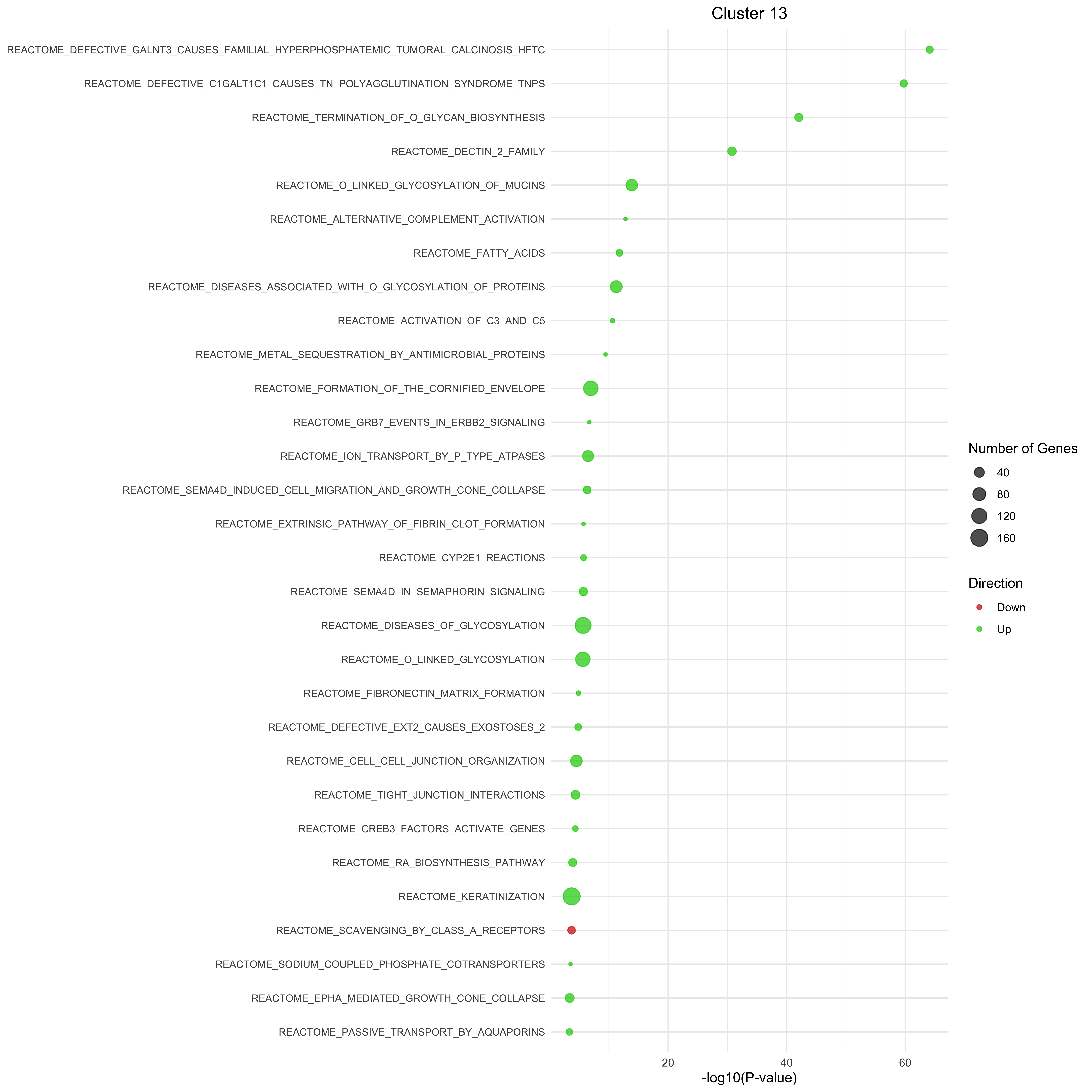
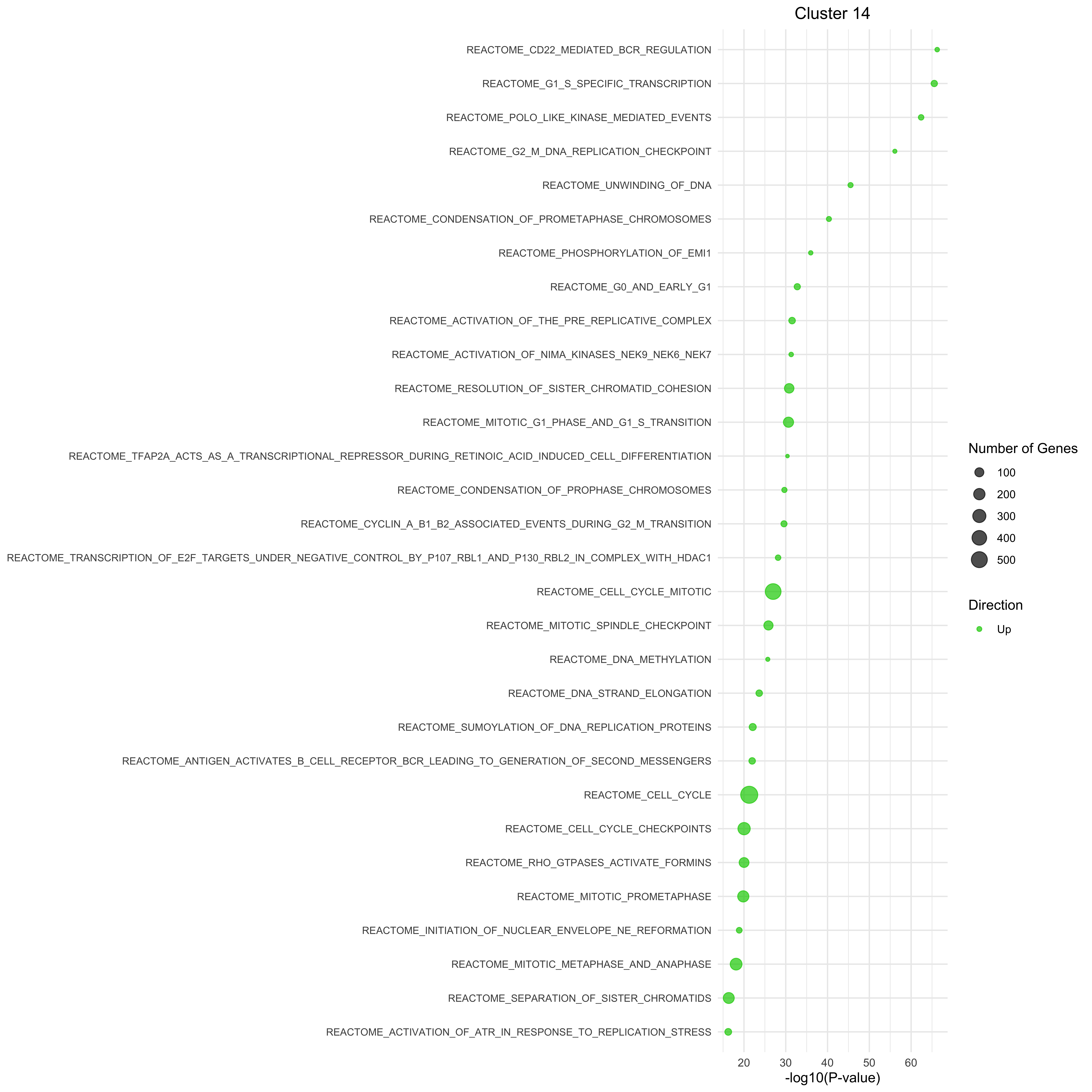
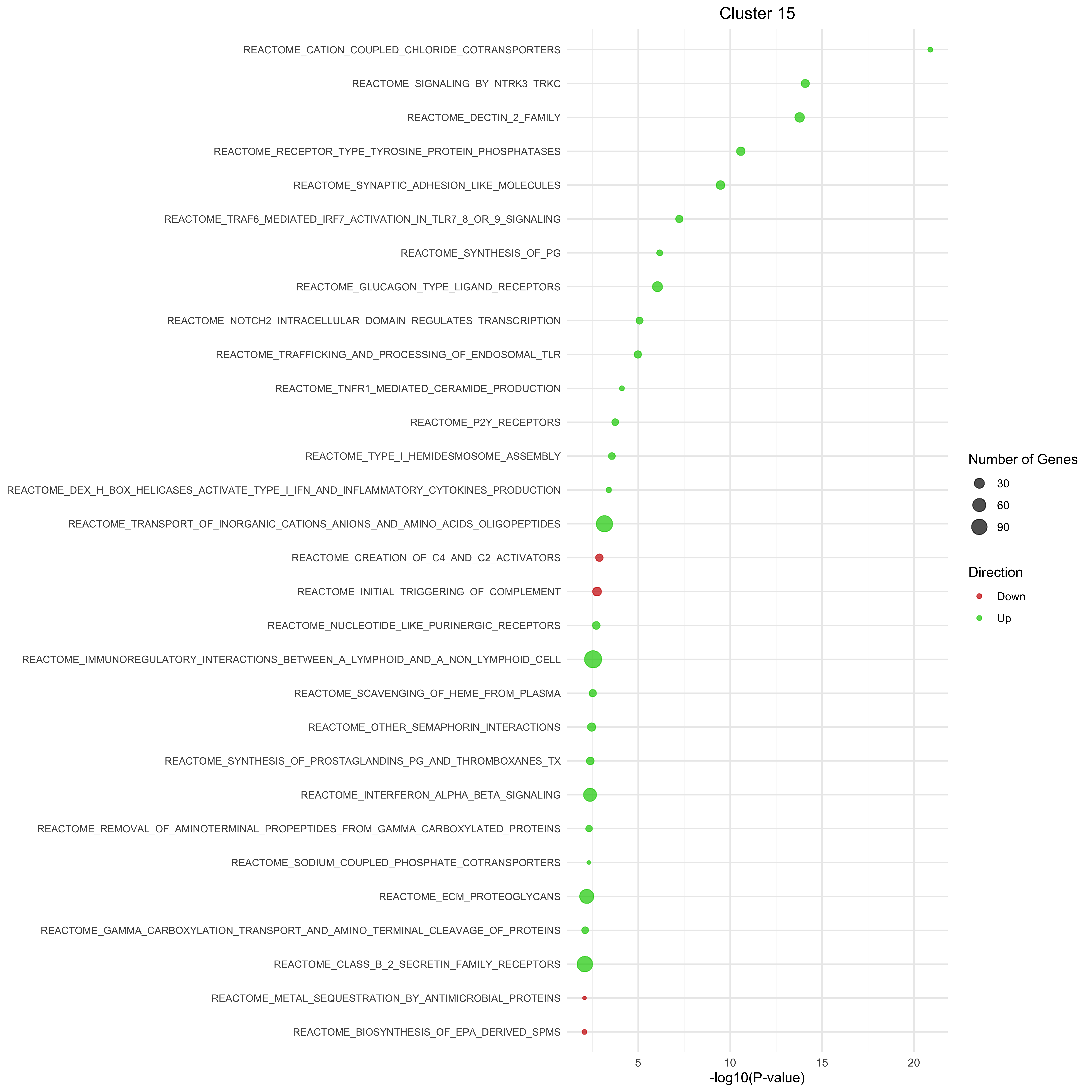
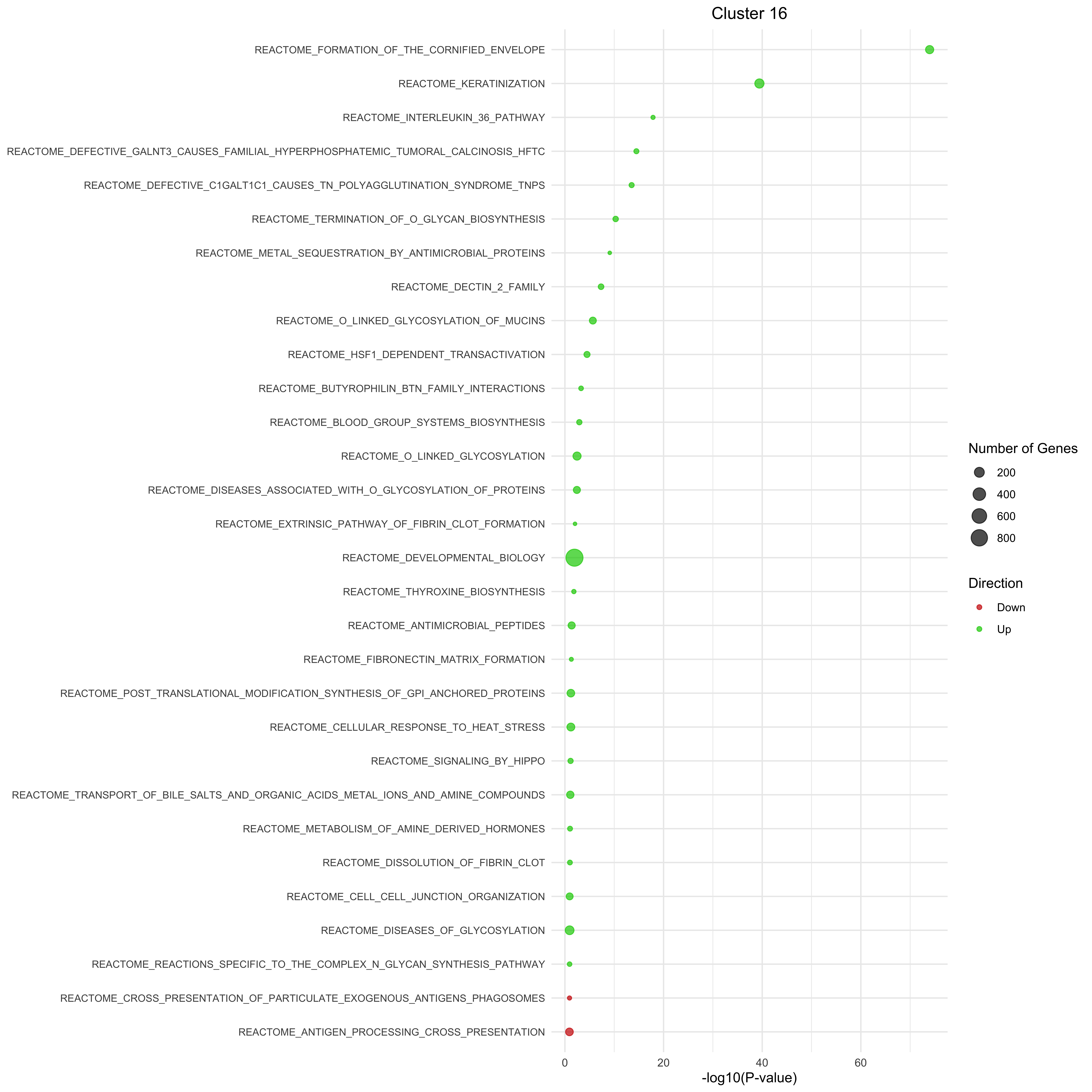
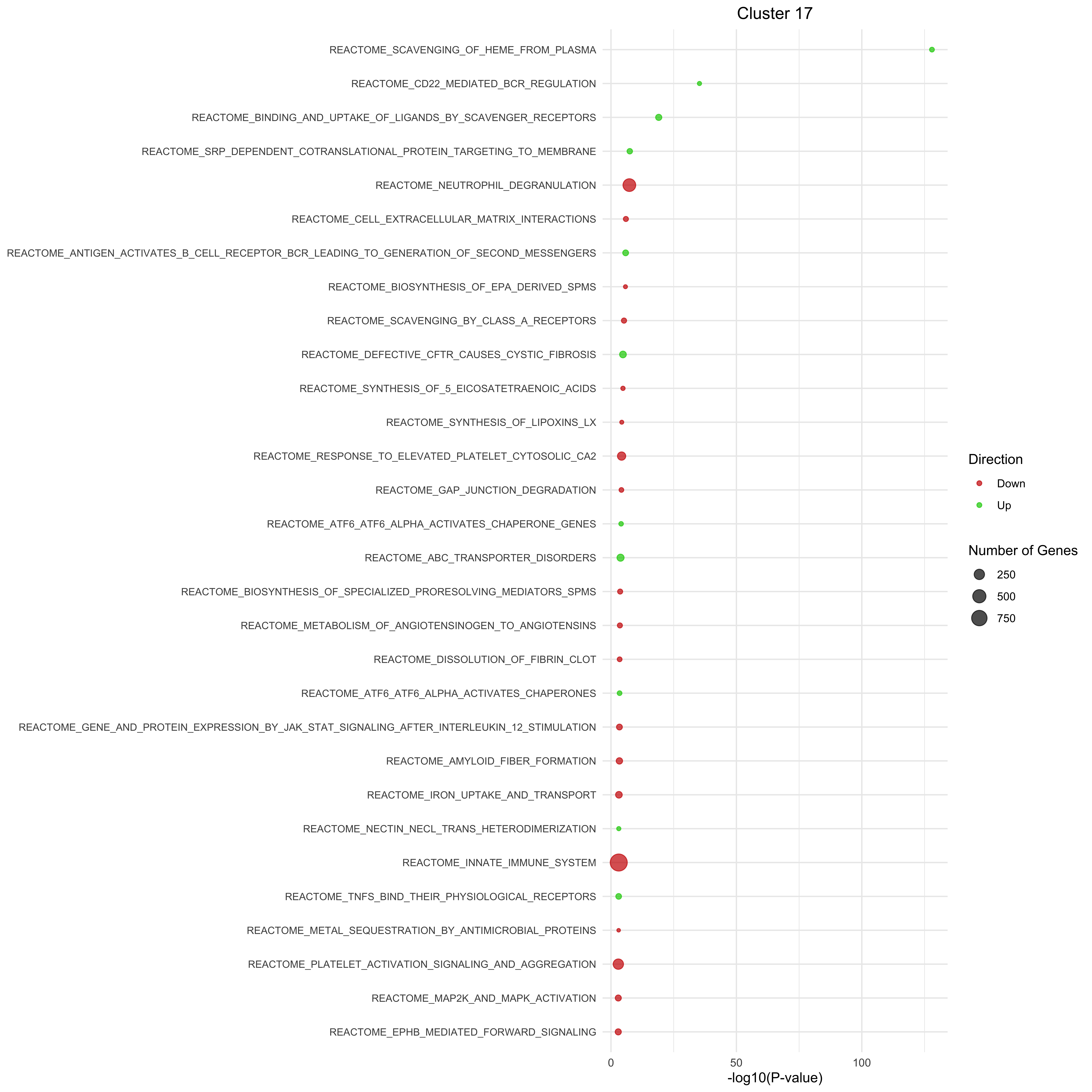
NOTE: Cluster 12: Unknown

Updated cell-type labels

cell_labels <- readxl::read_excel(here("data/Cell_labels_Mel/earlyAIR_BAL_annotations_02.05.24.xlsx"))
new_cluster_names <- cell_labels %>% 
  dplyr::select(cluster, annotation) %>% 
  deframe()

seu_obj <- RenameIdents(seu_obj, new_cluster_names)
seu_obj@meta.data$cell_labels <- Idents(seu_obj)

p3 <- DimPlot(seu_obj, reduction = "umap", raster = FALSE, repel = TRUE, label = TRUE, label.size = 3.5) + ggtitle(paste0(tissue, ": UMAP with Updated cell types"))

p1 / p3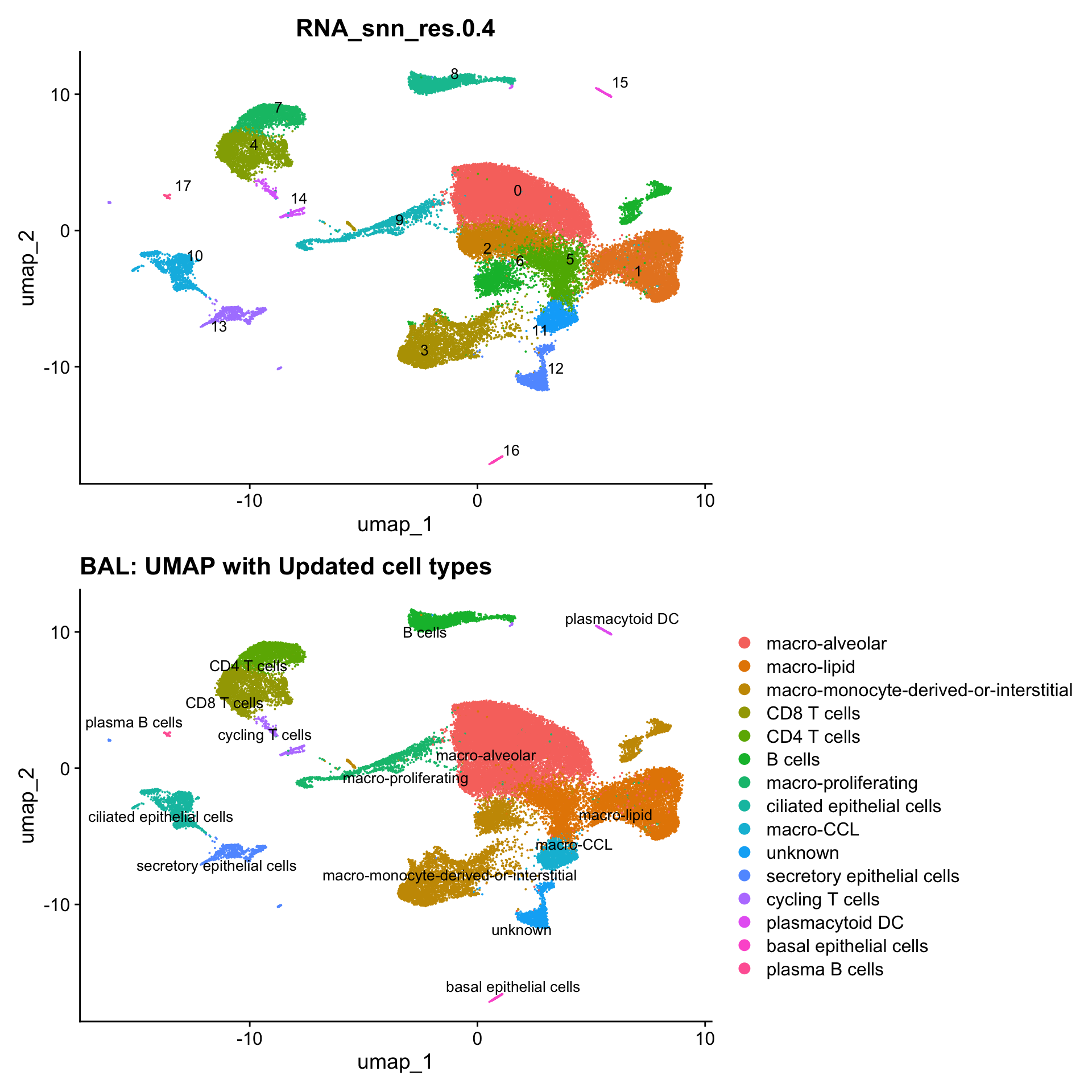

Past versions of unnamed-chunk-9-1.png

Version	Author	Date
77c742e	Gunjan Dixit	2024-06-26
e0e83af	Gunjan Dixit	2024-06-04

p3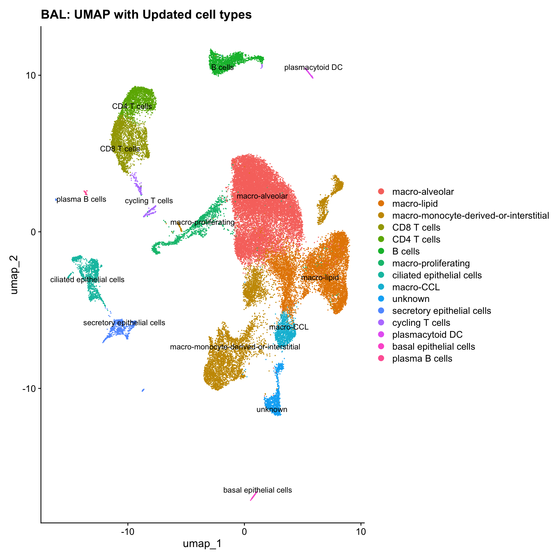

Past versions of unnamed-chunk-9-2.png

Version	Author	Date
77c742e	Gunjan Dixit	2024-06-26
e0e83af	Gunjan Dixit	2024-06-04

seu_obj@meta.data %>%
  ggplot(aes(x = cell_labels, fill = cell_labels)) +
  geom_bar() +
  geom_text(aes(label = ..count..), stat = "count",
            vjust = -0.5, colour = "black", size = 2) +
  theme(axis.text.x = element_text(angle = 90, vjust = 0.5, hjust = 1)) +
  NoLegend() + ggtitle(paste0(tissue, " : Counts per cell-type"))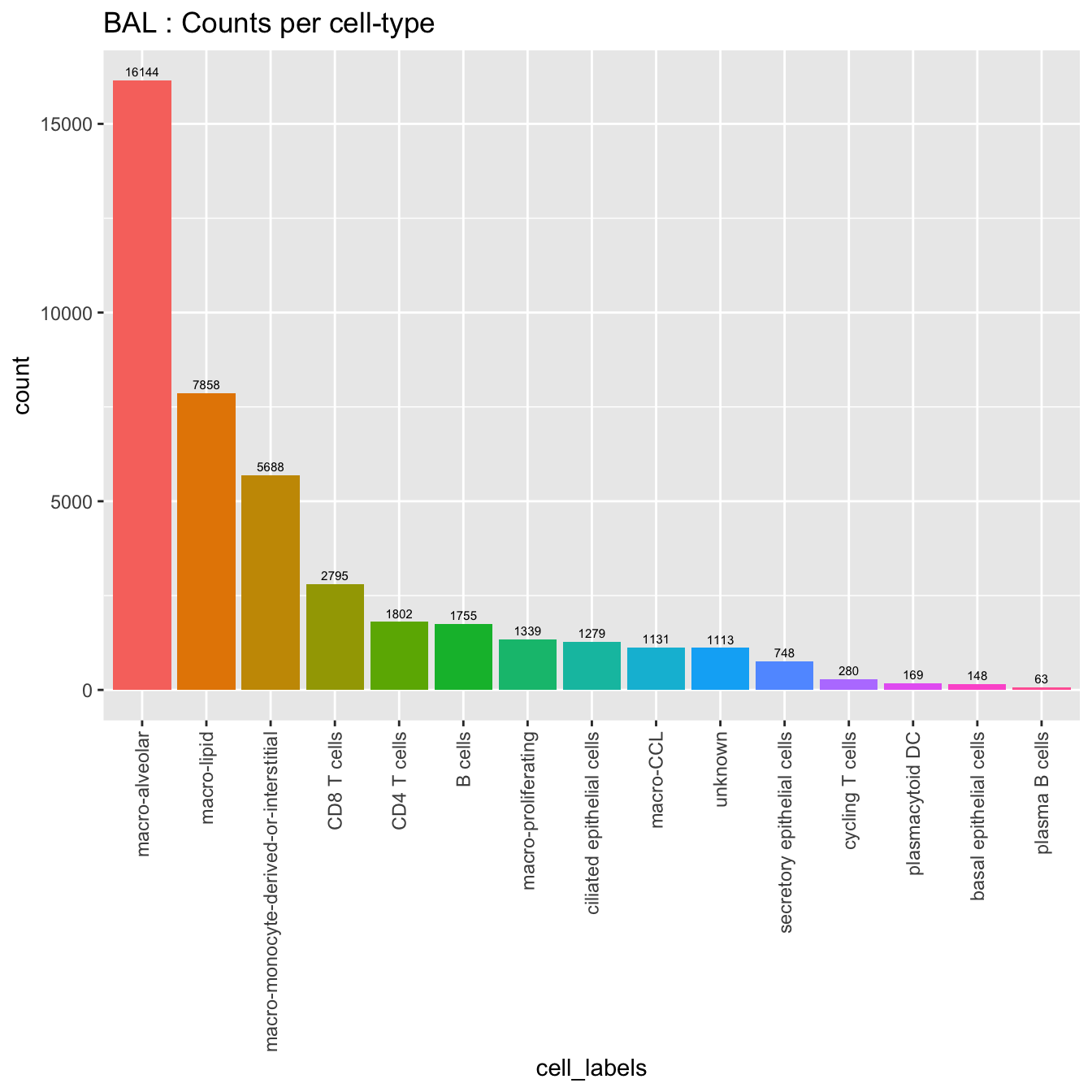

Past versions of unnamed-chunk-10-1.png

Version	Author	Date
e0e83af	Gunjan Dixit	2024-06-04

Reclustering Macro polulation

The marker genes for this reclustering can be found here-

BAL_Macro_population_res.0.7

idx <- which(Idents(seu_obj) %in% c("macro-monocyte-derived-or-interstitial", "macro-proliferating", "macro-lipid", "macro-alveolar", "macro-CCL"))
paed_sub <- seu_obj[,idx]
mito_genes <- grep("^MT-", rownames(paed_sub), value = TRUE)
paed_sub@meta.data$donor <- sub("_\\d+$", "", paed_sub@meta.data$Sample)
paed_sub <- subset(paed_sub, features = setdiff(rownames(paed_sub), mito_genes))
paed_sub

An object of class Seurat 
17518 features across 32160 samples within 1 assay 
Active assay: RNA (17518 features, 1990 variable features)
 3 layers present: counts, data, scale.data
 3 dimensional reductions calculated: pca, umap, umap.unintegrated

paed_sub <- paed_sub %>%
  NormalizeData() %>%
  FindVariableFeatures() %>%
  ScaleData() %>%
  RunPCA() 
  
paed_sub <- RunUMAP(paed_sub, dims = 1:30, reduction = "pca", reduction.name = "umap.new")

meta_data_columns <- colnames(paed_sub@meta.data)
columns_to_remove <- grep("^RNA_snn_res", meta_data_columns, value = TRUE)
paed_sub@meta.data <- paed_sub@meta.data[, !(colnames(paed_sub@meta.data) %in% columns_to_remove)]


resolutions <- seq(0.1, 1, by = 0.1)
paed_sub <- FindNeighbors(paed_sub, reduction = "pca", dims = 1:30)
paed_sub <- FindClusters(paed_sub, resolution = resolutions, algorithm = 3)

Modularity Optimizer version 1.3.0 by Ludo Waltman and Nees Jan van Eck

Number of nodes: 32160
Number of edges: 1020809

Running smart local moving algorithm...
Maximum modularity in 10 random starts: 0.9661
Number of communities: 8
Elapsed time: 25 seconds
Modularity Optimizer version 1.3.0 by Ludo Waltman and Nees Jan van Eck

Number of nodes: 32160
Number of edges: 1020809

Running smart local moving algorithm...
Maximum modularity in 10 random starts: 0.9505
Number of communities: 9
Elapsed time: 25 seconds
Modularity Optimizer version 1.3.0 by Ludo Waltman and Nees Jan van Eck

Number of nodes: 32160
Number of edges: 1020809

Running smart local moving algorithm...
Maximum modularity in 10 random starts: 0.9356
Number of communities: 11
Elapsed time: 24 seconds
Modularity Optimizer version 1.3.0 by Ludo Waltman and Nees Jan van Eck

Number of nodes: 32160
Number of edges: 1020809

Running smart local moving algorithm...
Maximum modularity in 10 random starts: 0.9215
Number of communities: 15
Elapsed time: 23 seconds
Modularity Optimizer version 1.3.0 by Ludo Waltman and Nees Jan van Eck

Number of nodes: 32160
Number of edges: 1020809

Running smart local moving algorithm...
Maximum modularity in 10 random starts: 0.9121
Number of communities: 18
Elapsed time: 22 seconds
Modularity Optimizer version 1.3.0 by Ludo Waltman and Nees Jan van Eck

Number of nodes: 32160
Number of edges: 1020809

Running smart local moving algorithm...
Maximum modularity in 10 random starts: 0.9039
Number of communities: 18
Elapsed time: 21 seconds
Modularity Optimizer version 1.3.0 by Ludo Waltman and Nees Jan van Eck

Number of nodes: 32160
Number of edges: 1020809

Running smart local moving algorithm...
Maximum modularity in 10 random starts: 0.8958
Number of communities: 18
Elapsed time: 21 seconds
Modularity Optimizer version 1.3.0 by Ludo Waltman and Nees Jan van Eck

Number of nodes: 32160
Number of edges: 1020809

Running smart local moving algorithm...
Maximum modularity in 10 random starts: 0.8877
Number of communities: 19
Elapsed time: 20 seconds
Modularity Optimizer version 1.3.0 by Ludo Waltman and Nees Jan van Eck

Number of nodes: 32160
Number of edges: 1020809

Running smart local moving algorithm...
Maximum modularity in 10 random starts: 0.8805
Number of communities: 20
Elapsed time: 19 seconds
Modularity Optimizer version 1.3.0 by Ludo Waltman and Nees Jan van Eck

Number of nodes: 32160
Number of edges: 1020809

Running smart local moving algorithm...
Maximum modularity in 10 random starts: 0.8735
Number of communities: 21
Elapsed time: 19 seconds

DimHeatmap(paed_sub, dims = 1:10, cells = 500, balanced = TRUE)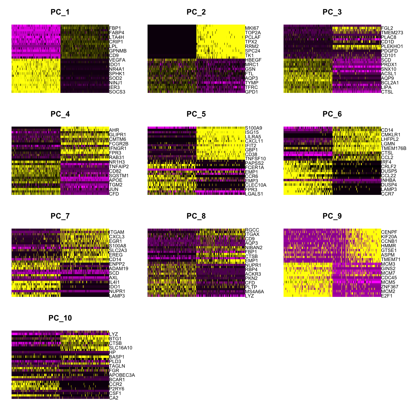

Past versions of unnamed-chunk-12-1.png

Version	Author	Date
ec13ee8	Gunjan Dixit	2024-06-26
77c742e	Gunjan Dixit	2024-06-26

clustree(paed_sub, prefix = "RNA_snn_res.")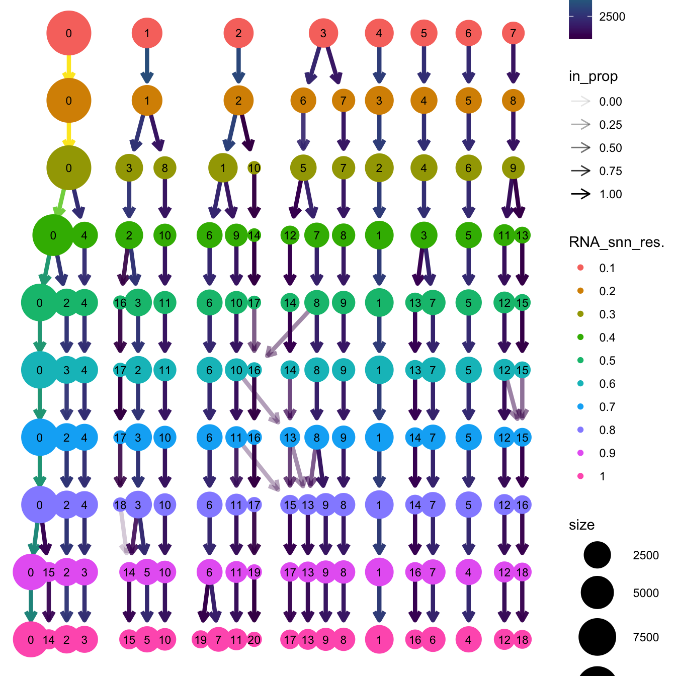

Past versions of unnamed-chunk-12-2.png

Version	Author	Date
ec13ee8	Gunjan Dixit	2024-06-26
77c742e	Gunjan Dixit	2024-06-26

opt_res <- "RNA_snn_res.0.7"  
n <- nlevels(paed_sub$RNA_snn_res.0.7)
paed_sub$RNA_snn_res.0.7 <- factor(paed_sub$RNA_snn_res.0.7, levels = seq(0,n-1))
paed_sub$seurat_clusters <- NULL
Idents(paed_sub) <- paed_sub$RNA_snn_res.0.7

DimPlot(paed_sub, reduction = "umap.new", group.by = "RNA_snn_res.0.7", label = TRUE, label.size = 4.5, repel = TRUE, raster = FALSE )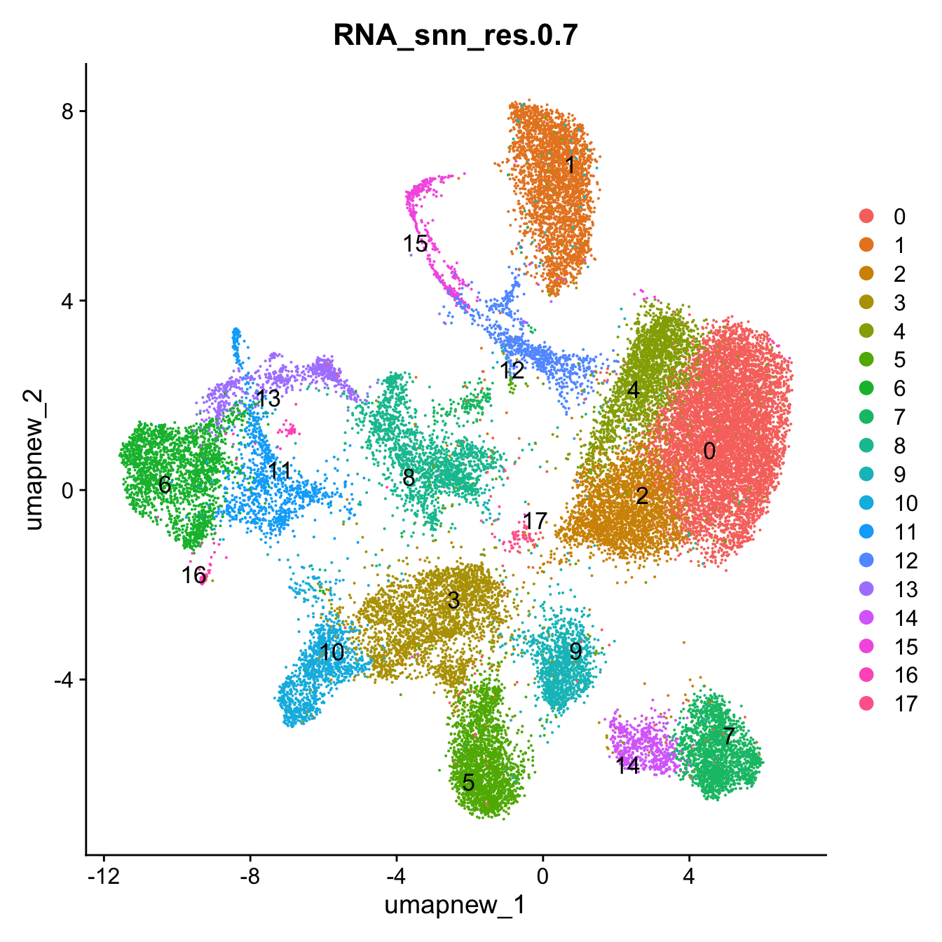

Past versions of unnamed-chunk-14-1.png

Version	Author	Date
0af5a78	Gunjan Dixit	2024-07-30
c20f60f	Gunjan Dixit	2024-07-08
ec13ee8	Gunjan Dixit	2024-06-26
77c742e	Gunjan Dixit	2024-06-26

DimPlot(paed_sub, reduction = "umap.new", group.by = "predicted.ann_finest_level", label = TRUE, label.size = 4.5, repel = TRUE, raster = FALSE )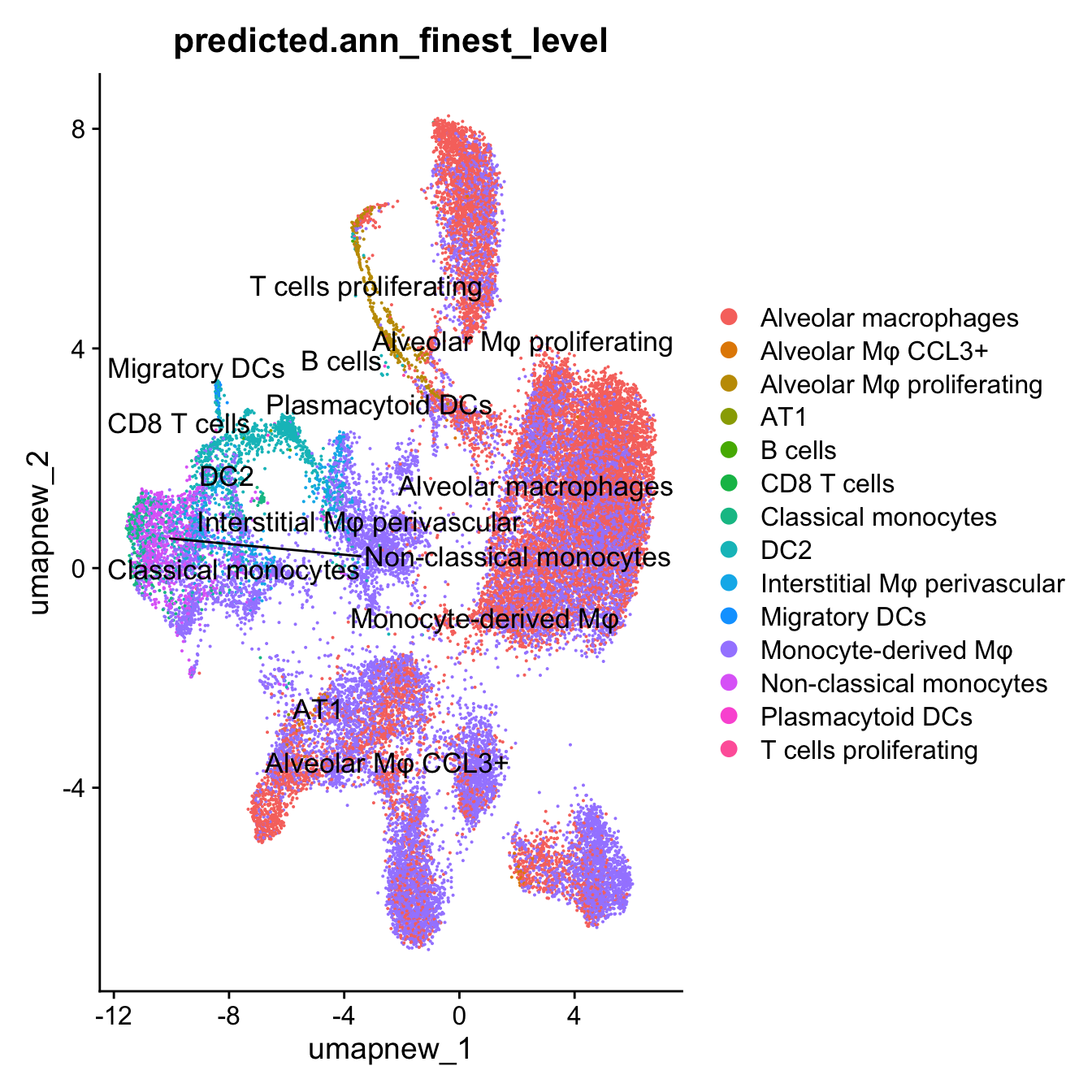

Past versions of unnamed-chunk-15-1.png

Version	Author	Date
0af5a78	Gunjan Dixit	2024-07-30
c20f60f	Gunjan Dixit	2024-07-08
ec13ee8	Gunjan Dixit	2024-06-26
77c742e	Gunjan Dixit	2024-06-26

DimPlot(paed_sub, reduction = "umap.new", group.by = "predicted.ann_level_3", label = TRUE, label.size = 4.5, repel = TRUE, raster = FALSE )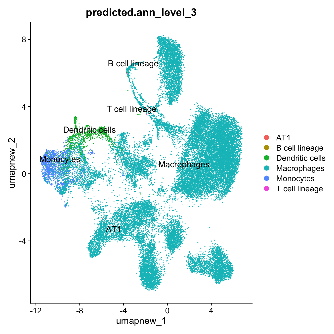

Past versions of unnamed-chunk-15-2.png

Version	Author	Date
0af5a78	Gunjan Dixit	2024-07-30

DimPlot(paed_sub, reduction = "umap.new", group.by = "predicted.ann_level_4", label = TRUE, label.size = 4.5, repel = TRUE, raster = FALSE )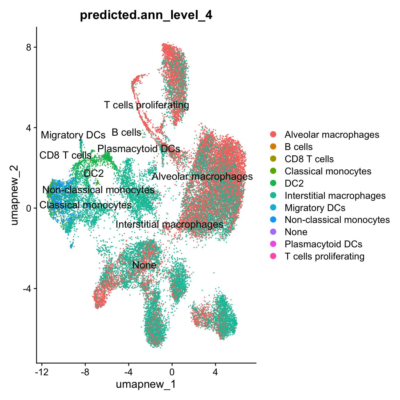

Past versions of unnamed-chunk-15-3.png

Version	Author	Date
0af5a78	Gunjan Dixit	2024-07-30

DimPlot(paed_sub, reduction = "umap.new", group.by = "predicted.ann_level_5", label = TRUE, label.size = 4.5, repel = TRUE, raster = FALSE )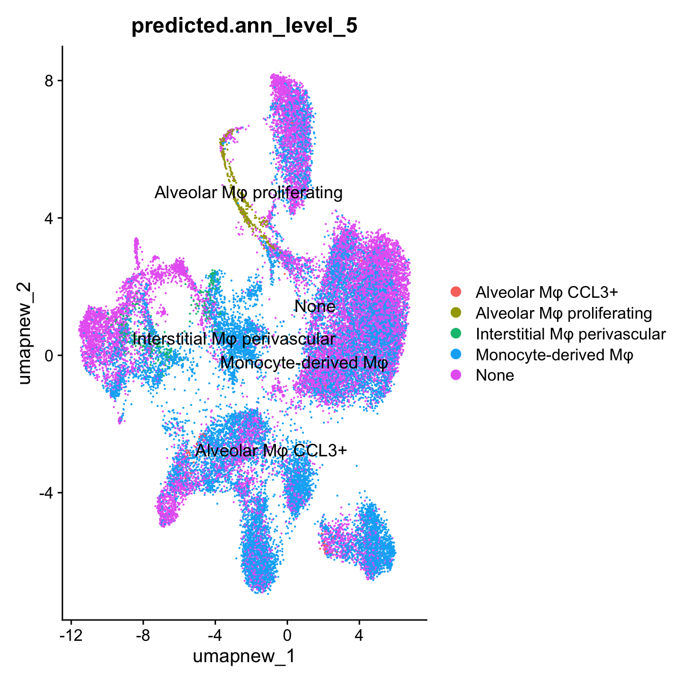

Past versions of unnamed-chunk-15-4.png

Version	Author	Date
0af5a78	Gunjan Dixit	2024-07-30

paed_sub.markers <- FindAllMarkers(paed_sub, only.pos = TRUE, min.pct = 0.25, logfc.threshold = 0.25)

Calculating cluster 0

Calculating cluster 1

Calculating cluster 2

Calculating cluster 3

Calculating cluster 4

Calculating cluster 5

Calculating cluster 6

Calculating cluster 7

Calculating cluster 8

Calculating cluster 9

Calculating cluster 10

Calculating cluster 11

Calculating cluster 12

Calculating cluster 13

Calculating cluster 14

Calculating cluster 15

Calculating cluster 16

Calculating cluster 17

paed_sub.markers %>%
    group_by(cluster) %>% unique() %>% 
    top_n(n = 10, wt = avg_log2FC) -> top10

paed_sub.markers %>%
    group_by(cluster) %>% 
    slice_head(n=1) %>% 
    pull(gene) -> best.wilcox.gene.per.cluster

best.wilcox.gene.per.cluster

 [1] "THBS1"    "DEFB1"    "APP"      "NR1H3"    "SENP3"    "PRDX2"   
 [7] "SERPINB9" "NRP2"     "VCAN"     "PLA1A"    "CXCL2"    "SOCS3"   
[13] "E2F1"     "CLEC10A"  "NRP2"     "MKI67"    "PROK2"    "TMSB4X"  

FeaturePlot(paed_sub,features=best.wilcox.gene.per.cluster, reduction = 'umap.new', raster = FALSE, label = T, ncol = 3)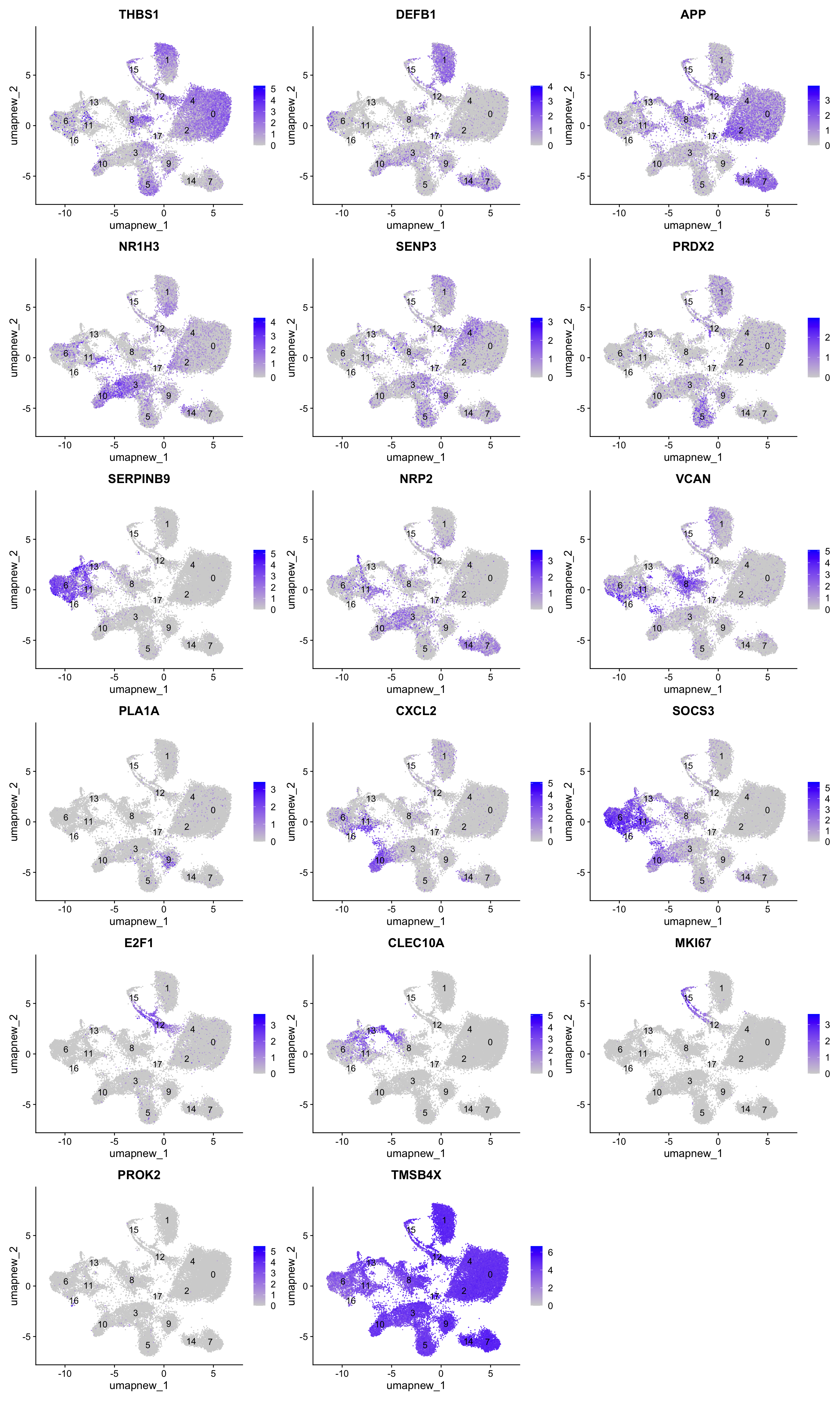

Past versions of unnamed-chunk-16-1.png

Version	Author	Date
0af5a78	Gunjan Dixit	2024-07-30

out_markers <- here("output",
            "CSV", 
            paste(tissue,"_Marker_genes_Reclustered_macro_population.",opt_res, sep = ""))

dir.create(out_markers, recursive = TRUE, showWarnings = FALSE)

for (cl in unique(paed_sub.markers$cluster)) {
  cluster_data <- paed_sub.markers %>% dplyr::filter(cluster == cl)
  file_name <- here(out_markers, paste0("G000231_Neeland_",tissue, "_cluster_", cl, ".csv"))
  write.csv(cluster_data, file = file_name)
}

Marker-analysis of Macro population using Limma

paed_sub@meta.data$donor <- sub("_\\d+$", "", paed_sub@meta.data$Sample)

logcounts <- normCounts(DGEList(as.matrix(paed_sub[["RNA"]]$counts)),
                        log = TRUE, prior.count = 0.5)

Warning in asMethod(object): sparse->dense coercion: allocating vector of size
4.2 GiB

entrez <- AnnotationDbi::mapIds(org.Hs.eg.db,
                                keys = rownames(logcounts),
                                column = c("ENTREZID"),
                                keytype = "SYMBOL",
                                multiVals = "first")

'select()' returned 1:many mapping between keys and columns

logcounts <- logcounts[!is.na(entrez),]

maxclust <- length(levels(Idents(paed_sub))) - 1

clustgrp <- paste0("c", Idents(paed_sub))
clustgrp <- factor(clustgrp, levels = paste0("c", 0:maxclust))
sample <- paed_sub$donor

design <- model.matrix(~ 0 + clustgrp + sample)
colnames(design)[1:(length(levels(clustgrp)))] <- levels(clustgrp)

head(design)

  c0 c1 c2 c3 c4 c5 c6 c7 c8 c9 c10 c11 c12 c13 c14 c15 c16 c17 sampleeAIR035
1  0  1  0  0  0  0  0  0  0  0   0   0   0   0   0   0   0   0             0
2  0  1  0  0  0  0  0  0  0  0   0   0   0   0   0   0   0   0             0
3  0  1  0  0  0  0  0  0  0  0   0   0   0   0   0   0   0   0             0
4  0  1  0  0  0  0  0  0  0  0   0   0   0   0   0   0   0   0             0
5  0  1  0  0  0  0  0  0  0  0   0   0   0   0   0   0   0   0             0
6  0  0  0  0  0  0  0  0  0  0   0   0   0   0   0   1   0   0             0
  sampleeAIR036 sampleeAIR045 sampleeAIR046 sampleeAIR054 sampleeAIR057
1             0             0             0             0             0
2             0             0             0             0             0
3             0             0             0             0             0
4             0             0             0             0             0
5             0             0             0             0             0
6             0             0             0             0             0
  sampleeAIR059
1             0
2             0
3             0
4             0
5             0
6             0

# Create contrast matrix
mycont <- matrix(NA, ncol = length(levels(clustgrp)),
                 nrow = length(levels(clustgrp)))
rownames(mycont) <- colnames(mycont) <- levels(clustgrp)
diag(mycont) <- 1
mycont[upper.tri(mycont)] <- -1/(length(levels(factor(clustgrp))) - 1)
mycont[lower.tri(mycont)] <- -1/(length(levels(factor(clustgrp))) - 1)
mycont

            c0         c1         c2         c3         c4         c5
c0   1.0000000 -0.0588235 -0.0588235 -0.0588235 -0.0588235 -0.0588235
c1  -0.0588235  1.0000000 -0.0588235 -0.0588235 -0.0588235 -0.0588235
c2  -0.0588235 -0.0588235  1.0000000 -0.0588235 -0.0588235 -0.0588235
c3  -0.0588235 -0.0588235 -0.0588235  1.0000000 -0.0588235 -0.0588235
c4  -0.0588235 -0.0588235 -0.0588235 -0.0588235  1.0000000 -0.0588235
c5  -0.0588235 -0.0588235 -0.0588235 -0.0588235 -0.0588235  1.0000000
c6  -0.0588235 -0.0588235 -0.0588235 -0.0588235 -0.0588235 -0.0588235
c7  -0.0588235 -0.0588235 -0.0588235 -0.0588235 -0.0588235 -0.0588235
c8  -0.0588235 -0.0588235 -0.0588235 -0.0588235 -0.0588235 -0.0588235
c9  -0.0588235 -0.0588235 -0.0588235 -0.0588235 -0.0588235 -0.0588235
c10 -0.0588235 -0.0588235 -0.0588235 -0.0588235 -0.0588235 -0.0588235
c11 -0.0588235 -0.0588235 -0.0588235 -0.0588235 -0.0588235 -0.0588235
c12 -0.0588235 -0.0588235 -0.0588235 -0.0588235 -0.0588235 -0.0588235
c13 -0.0588235 -0.0588235 -0.0588235 -0.0588235 -0.0588235 -0.0588235
c14 -0.0588235 -0.0588235 -0.0588235 -0.0588235 -0.0588235 -0.0588235
c15 -0.0588235 -0.0588235 -0.0588235 -0.0588235 -0.0588235 -0.0588235
c16 -0.0588235 -0.0588235 -0.0588235 -0.0588235 -0.0588235 -0.0588235
c17 -0.0588235 -0.0588235 -0.0588235 -0.0588235 -0.0588235 -0.0588235
            c6         c7         c8         c9        c10        c11
c0  -0.0588235 -0.0588235 -0.0588235 -0.0588235 -0.0588235 -0.0588235
c1  -0.0588235 -0.0588235 -0.0588235 -0.0588235 -0.0588235 -0.0588235
c2  -0.0588235 -0.0588235 -0.0588235 -0.0588235 -0.0588235 -0.0588235
c3  -0.0588235 -0.0588235 -0.0588235 -0.0588235 -0.0588235 -0.0588235
c4  -0.0588235 -0.0588235 -0.0588235 -0.0588235 -0.0588235 -0.0588235
c5  -0.0588235 -0.0588235 -0.0588235 -0.0588235 -0.0588235 -0.0588235
c6   1.0000000 -0.0588235 -0.0588235 -0.0588235 -0.0588235 -0.0588235
c7  -0.0588235  1.0000000 -0.0588235 -0.0588235 -0.0588235 -0.0588235
c8  -0.0588235 -0.0588235  1.0000000 -0.0588235 -0.0588235 -0.0588235
c9  -0.0588235 -0.0588235 -0.0588235  1.0000000 -0.0588235 -0.0588235
c10 -0.0588235 -0.0588235 -0.0588235 -0.0588235  1.0000000 -0.0588235
c11 -0.0588235 -0.0588235 -0.0588235 -0.0588235 -0.0588235  1.0000000
c12 -0.0588235 -0.0588235 -0.0588235 -0.0588235 -0.0588235 -0.0588235
c13 -0.0588235 -0.0588235 -0.0588235 -0.0588235 -0.0588235 -0.0588235
c14 -0.0588235 -0.0588235 -0.0588235 -0.0588235 -0.0588235 -0.0588235
c15 -0.0588235 -0.0588235 -0.0588235 -0.0588235 -0.0588235 -0.0588235
c16 -0.0588235 -0.0588235 -0.0588235 -0.0588235 -0.0588235 -0.0588235
c17 -0.0588235 -0.0588235 -0.0588235 -0.0588235 -0.0588235 -0.0588235
           c12        c13        c14        c15        c16        c17
c0  -0.0588235 -0.0588235 -0.0588235 -0.0588235 -0.0588235 -0.0588235
c1  -0.0588235 -0.0588235 -0.0588235 -0.0588235 -0.0588235 -0.0588235
c2  -0.0588235 -0.0588235 -0.0588235 -0.0588235 -0.0588235 -0.0588235
c3  -0.0588235 -0.0588235 -0.0588235 -0.0588235 -0.0588235 -0.0588235
c4  -0.0588235 -0.0588235 -0.0588235 -0.0588235 -0.0588235 -0.0588235
c5  -0.0588235 -0.0588235 -0.0588235 -0.0588235 -0.0588235 -0.0588235
c6  -0.0588235 -0.0588235 -0.0588235 -0.0588235 -0.0588235 -0.0588235
c7  -0.0588235 -0.0588235 -0.0588235 -0.0588235 -0.0588235 -0.0588235
c8  -0.0588235 -0.0588235 -0.0588235 -0.0588235 -0.0588235 -0.0588235
c9  -0.0588235 -0.0588235 -0.0588235 -0.0588235 -0.0588235 -0.0588235
c10 -0.0588235 -0.0588235 -0.0588235 -0.0588235 -0.0588235 -0.0588235
c11 -0.0588235 -0.0588235 -0.0588235 -0.0588235 -0.0588235 -0.0588235
c12  1.0000000 -0.0588235 -0.0588235 -0.0588235 -0.0588235 -0.0588235
c13 -0.0588235  1.0000000 -0.0588235 -0.0588235 -0.0588235 -0.0588235
c14 -0.0588235 -0.0588235  1.0000000 -0.0588235 -0.0588235 -0.0588235
c15 -0.0588235 -0.0588235 -0.0588235  1.0000000 -0.0588235 -0.0588235
c16 -0.0588235 -0.0588235 -0.0588235 -0.0588235  1.0000000 -0.0588235
c17 -0.0588235 -0.0588235 -0.0588235 -0.0588235 -0.0588235  1.0000000

# Fill out remaining rows with 0s
zero.rows <- matrix(0, ncol = length(levels(clustgrp)),
                    nrow = (ncol(design) - length(levels(clustgrp))))
fullcont <- rbind(mycont, zero.rows)
rownames(fullcont) <- colnames(design)

fit <- lmFit(logcounts, design)

fit.cont <- contrasts.fit(fit, contrasts = fullcont)
fit.cont <- eBayes(fit.cont, trend = TRUE, robust = TRUE)

Warning: 2233 very small variances detected, have been offset away from zero

summary(decideTests(fit.cont))

          c0    c1    c2    c3    c4    c5    c6    c7    c8    c9   c10   c11
Down    2851  1462  2185  1572  1194  1432  8242  1405  2855  1193  2121  5726
NotSig 11300 11435 11419 12200  9311 12279  7103 11554 11675 11326 13173  9060
Up      2960  4214  3507  3339  6606  3400  1766  4152  2581  4592  1817  2325
         c12   c13   c14   c15   c16   c17
Down    1095  4218  1065  1136  5477  4738
NotSig 11392 10052 12769 11430 10915 12255
Up      4624  2841  3277  4545   719   118

Test relative to a threshold (TREAT)

#tr <- treat(fit.cont, fc=1.1) #10% fold change from documentation
tr <- treat(fit.cont, lfc=0.25)
dt <- decideTests(tr)
summary(dt)

          c0    c1    c2    c3    c4    c5    c6    c7    c8    c9   c10   c11
Down     104    62   106    91    56   144  1472    84   236    98   119   825
NotSig 16623 16549 16484 16754 16525 16564 15154 16401 16691 16541 16672 15836
Up       384   500   521   266   530   403   485   626   184   472   320   450
         c12   c13   c14   c15   c16   c17
Down      84   860    47   137  1492   853
NotSig 16446 15700 16575 16210 15391 16254
Up       581   551   489   764   228     4

Mean-difference plots per cluster

par(mfrow=c(4,3))
par(mar=c(2,3,1,2))

for(i in 1:ncol(mycont)){
  plotMD(tr, coef = i, status = dt[,i], hl.cex = 0.5)
  abline(h = 0, col = "lightgrey")
  lines(lowess(tr$Amean, tr$coefficients[,i]), lwd = 1.5, col = 4)
}

Past versions of unnamed-chunk-22-1.png

Version	Author	Date
0af5a78	Gunjan Dixit	2024-07-30
75b471c	Gunjan Dixit	2024-06-28
324c175	Gunjan Dixit	2024-06-28

Past versions of unnamed-chunk-22-2.png

Version	Author	Date
0af5a78	Gunjan Dixit	2024-07-30

Marker-gene dot plot

#Top 10 marker genes from limma analysis
DefaultAssay(paed_sub) <- "RNA"

contnames <- colnames(mycont)
top_markers <- NULL
n_markers <- 10
limma_markers_by_cluster <- vector("list", length = length(contnames))
names(limma_markers_by_cluster) <- contnames

for (i in seq_along(contnames)) {
  top <- topTreat(tr, coef = i, n = Inf)
  top <- top[top$logFC > 0.25, ]  # Filter for significant markers
  
  top_markers <- c(top_markers, 
                   setNames(rownames(top)[1:n_markers], 
                            rep(contnames[i], n_markers)))
  markers <- rownames(top)
  limma_markers_by_cluster[[contnames[i]]] <- markers
}

# Remove NA and duplicate markers
top_markers <- top_markers[!is.na(top_markers)]
top_markers <- top_markers[!duplicated(top_markers)]

cols <- paletteer::paletteer_d("pals::glasbey")[factor(names(top_markers))]

DotPlot(paed_sub,    
        features = unname(top_markers),
        group.by = opt_res,
        cols = c("azure1", "blueviolet"),
        dot.scale = 3, assay = "RNA") +
    RotatedAxis() +
    FontSize(y.text = 8, x.text = 12) +
    labs(y = element_blank(), x = element_blank()) +
    coord_flip() +
  theme(axis.text.y = element_text(color = cols)) +
  ggtitle("Top 10 cluster marker genes (Limma)")

Warning: Vectorized input to `element_text()` is not officially supported.
ℹ Results may be unexpected or may change in future versions of ggplot2.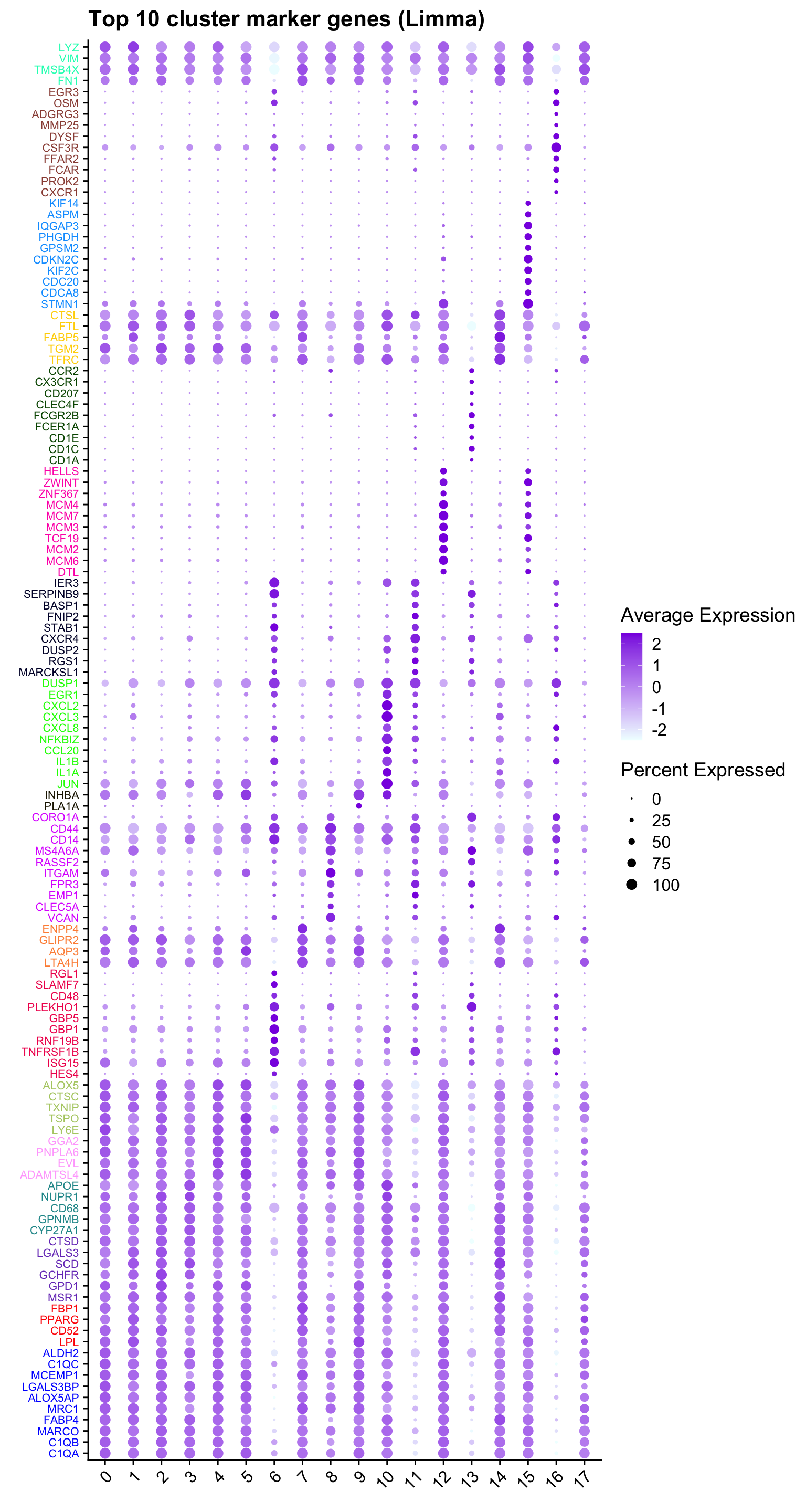

Past versions of unnamed-chunk-23-1.png

Version	Author	Date
0af5a78	Gunjan Dixit	2024-07-30
c20f60f	Gunjan Dixit	2024-07-08
324c175	Gunjan Dixit	2024-06-28

Top 10 marker genes from Seurat

## Seurat top markers
top10 <- paed_sub.markers %>%
    group_by(cluster) %>%
    top_n(n = 10, wt = avg_log2FC) %>%
    ungroup() %>%
    distinct(gene, .keep_all = TRUE) %>%
    arrange(cluster, desc(avg_log2FC))

cluster_colors <- paletteer::paletteer_d("pals::glasbey")[factor(top10$cluster)]

DotPlot(paed_sub,    
        features = unique(top10$gene),
        group.by = opt_res,
        cols = c("azure1", "blueviolet"),
        dot.scale = 3, assay = "RNA") +
    RotatedAxis() +
    FontSize(y.text = 8, x.text = 12) +
    labs(y = element_blank(), x = element_blank()) +
    coord_flip() +
    theme(axis.text.y = element_text(color = cluster_colors)) +
    ggtitle("Top 10 marker genes per cluster (Seurat)")

Warning: Vectorized input to `element_text()` is not officially supported.
ℹ Results may be unexpected or may change in future versions of ggplot2.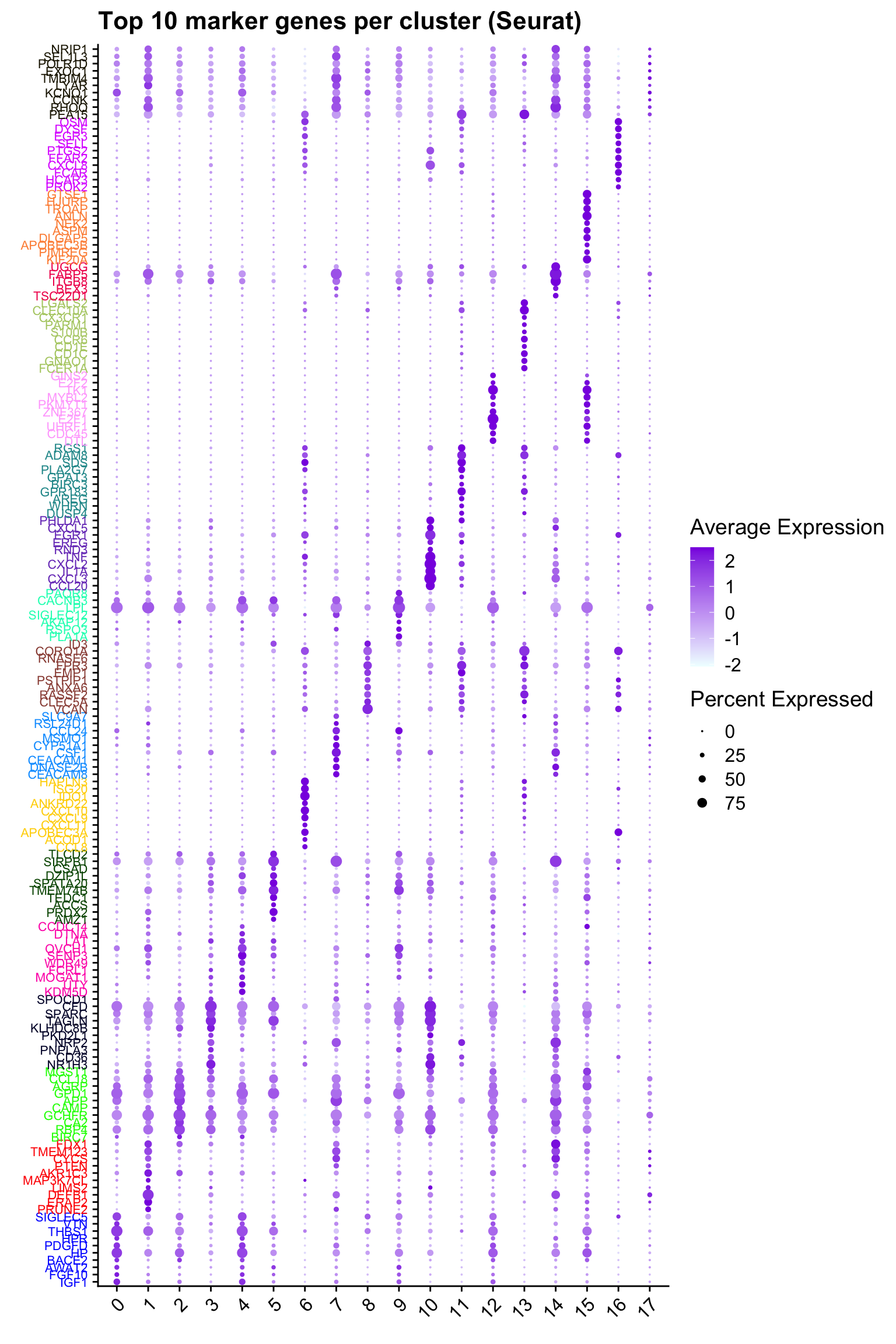

Past versions of unnamed-chunk-24-1.png

Version	Author	Date
0af5a78	Gunjan Dixit	2024-07-30
324c175	Gunjan Dixit	2024-06-28

df_table <- as.data.frame(table(paed_sub$RNA_snn_res.0.1, paed_sub$predicted.ann_finest_level))
ggplot(df_table, aes(Var1, Freq, fill = Var2)) +
  geom_bar(stat = "identity") +
  labs(x = "RNA_snn_res.0.1", y = "Count", fill = "predicted ann_finest_level") +
  theme_minimal() +
  ggtitle("Stacked Bar Plot of predicted.ann_finest_level")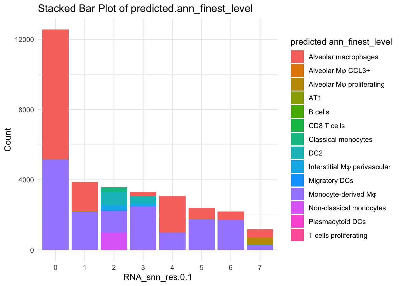

Past versions of unnamed-chunk-25-1.png

Version	Author	Date
0af5a78	Gunjan Dixit	2024-07-30

# Filter cells with >= 10 counts
valid_levels <- names(table(paed_sub$predicted.ann_finest_level)[table(paed_sub$predicted.ann_finest_level) >= 10])
paed_sub_filtered <- subset(paed_sub, subset = predicted.ann_finest_level %in% valid_levels)

# Stacked bar plot with filtered cells
df_table_filtered <- as.data.frame(table(paed_sub_filtered$RNA_snn_res.0.1, paed_sub_filtered$predicted.ann_finest_level))
ggplot(df_table_filtered, aes(x = Var1, y = Freq, fill = Var2)) +
    geom_bar(stat = "identity") +
    labs(x = "RNA_snn_res.0.1", y = "Count", fill = "predicted ann_finest_level") +
    theme_minimal() +
    ggtitle("Stacked Bar Plot of predicted.ann_finest_level")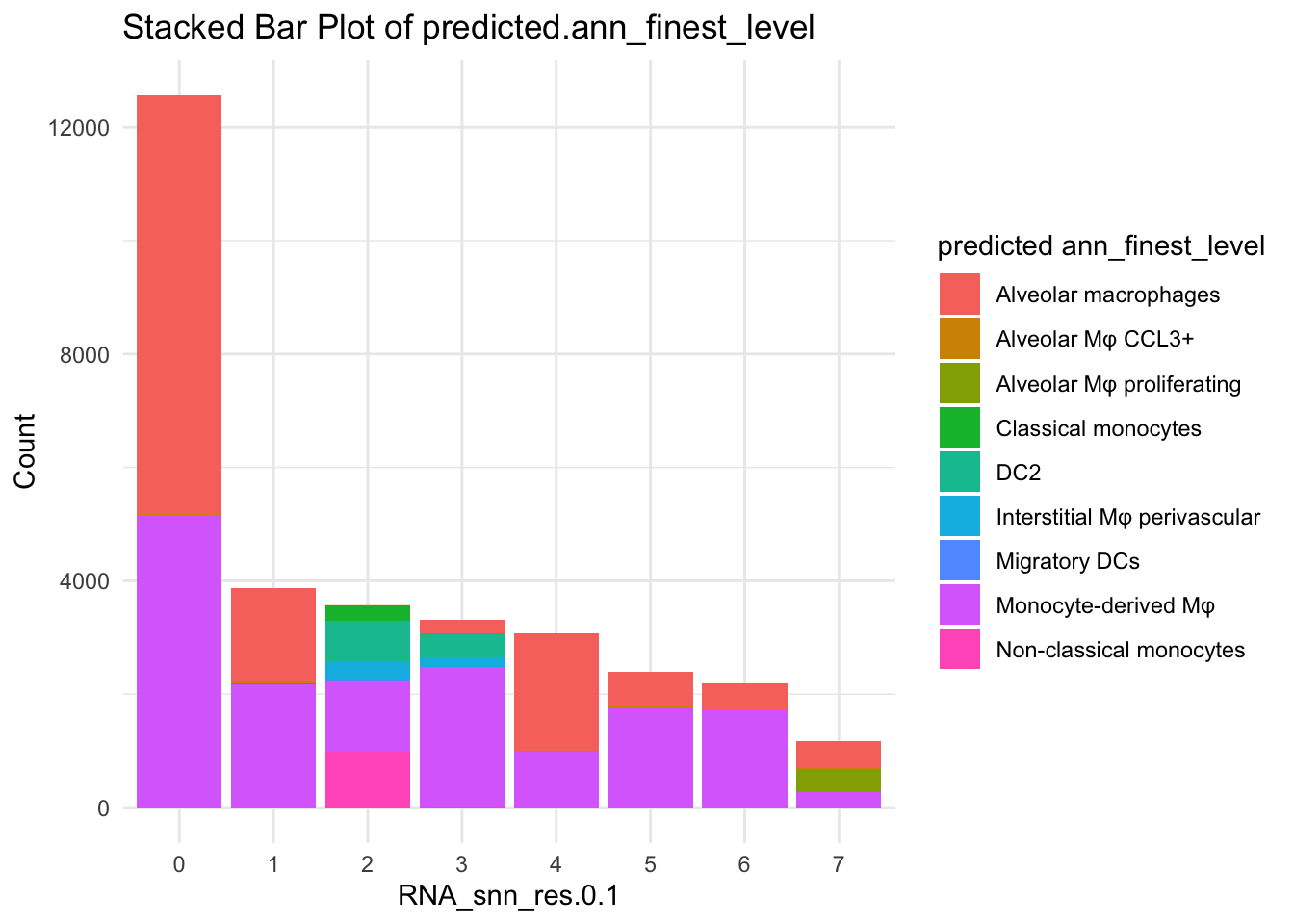

Past versions of unnamed-chunk-25-2.png

Version	Author	Date
0af5a78	Gunjan Dixit	2024-07-30

Overlapping and Unique markers between Seurat and Limma approach

limma_markers_by_cluster <- setNames(limma_markers_by_cluster, gsub("^c", "", names(limma_markers_by_cluster)))
limma_markers_df <- do.call(rbind, lapply(names(limma_markers_by_cluster), function(cluster) {
  data.frame(cluster = cluster, gene = limma_markers_by_cluster[[cluster]], stringsAsFactors = FALSE)
}))

seurat_markers_df <- paed_sub.markers[, c("cluster", "gene")]

marker_comparison_list <- list()
for (cluster in unique(names(limma_markers_by_cluster))) {
  limma_genes <- limma_markers_df$gene[limma_markers_df$cluster == cluster]
  seurat_genes <- seurat_markers_df$gene[seurat_markers_df$cluster == cluster]
  
  overlap <- intersect(limma_genes, seurat_genes)
  unique_limma <- setdiff(limma_genes, seurat_genes)
  unique_seurat <- setdiff(seurat_genes, limma_genes)
  
  marker_comparison_list[[cluster]] <- data.frame(
    Cluster = cluster,
    Category = c("Overlapping", "Unique Limma", "Unique Seurat"),
    Count = c(length(overlap), length(unique_limma), length(unique_seurat))
  )
}
marker_comparison_df <- do.call(rbind, marker_comparison_list)

marker_comparison_df$Cluster <- factor(marker_comparison_df$Cluster, levels = sort(as.numeric(unique(marker_comparison_df$Cluster))))

ggplot(marker_comparison_df, aes(x = Cluster, y = Count, fill = Category)) +
  geom_bar(stat = "identity", position = "stack") +
  theme_minimal() +
  labs(title = "Comparison of Marker Genes by Cluster (lfc: 0.25)",
       y = "Number of Genes",
       x = "Cluster") +
  scale_fill_manual(values = c("Overlapping" = "darkgreen", "Unique Limma" = "cornflowerblue", "Unique Seurat" = "darkorchid1"))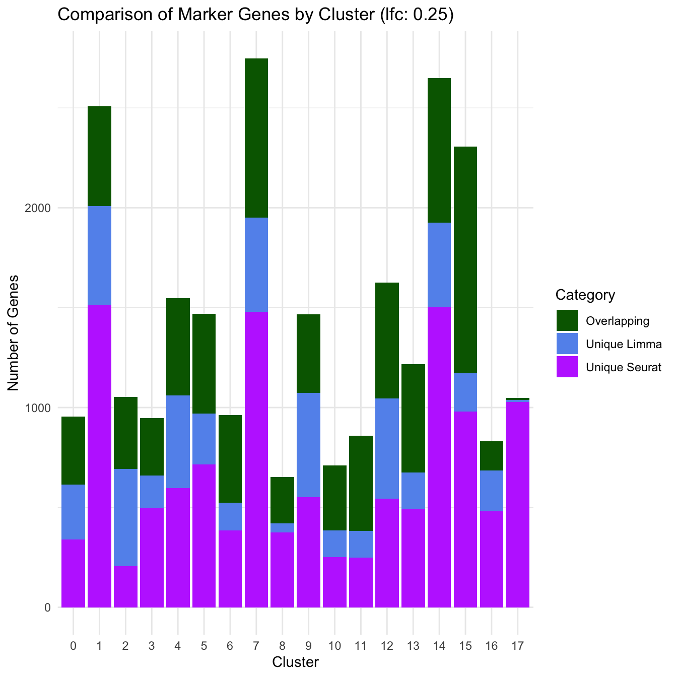

Past versions of unnamed-chunk-26-1.png

Version	Author	Date
0af5a78	Gunjan Dixit	2024-07-30
c20f60f	Gunjan Dixit	2024-07-08

Update Macro labels

cell_labels <- readxl::read_excel(here("data/Cell_labels_Mel_v2/earlyAIR_BAL_macrophage_reclustering_annotations_16.07.24.xlsx"))
new_cluster_names <- cell_labels %>% 
  dplyr::select(cluster, annotation) %>% 
  deframe()

paed_sub <- RenameIdents(paed_sub, new_cluster_names)
paed_sub@meta.data$cell_labels_v2 <- Idents(paed_sub)

DimPlot(paed_sub, reduction = "umap.new", raster = FALSE, repel = TRUE, label = TRUE, label.size = 3.5) + ggtitle(paste0(tissue, ": UMAP with Updated subclustering labels"))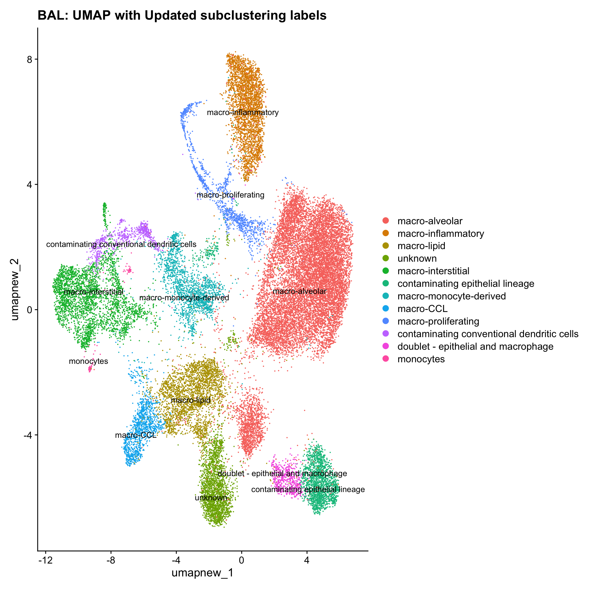

Past versions of unnamed-chunk-27-1.png

Version	Author	Date
0af5a78	Gunjan Dixit	2024-07-30
c20f60f	Gunjan Dixit	2024-07-08

Excluding contaminating labels

idx <- which(grepl("^contaminating", Idents(paed_sub)))
paed_clean <- paed_sub[, -idx]
DimPlot(paed_clean, reduction = "umap.new", raster = FALSE, repel = TRUE, label = TRUE, label.size = 3.5) + ggtitle(paste0(tissue, ":Updated subclustering (clean)"))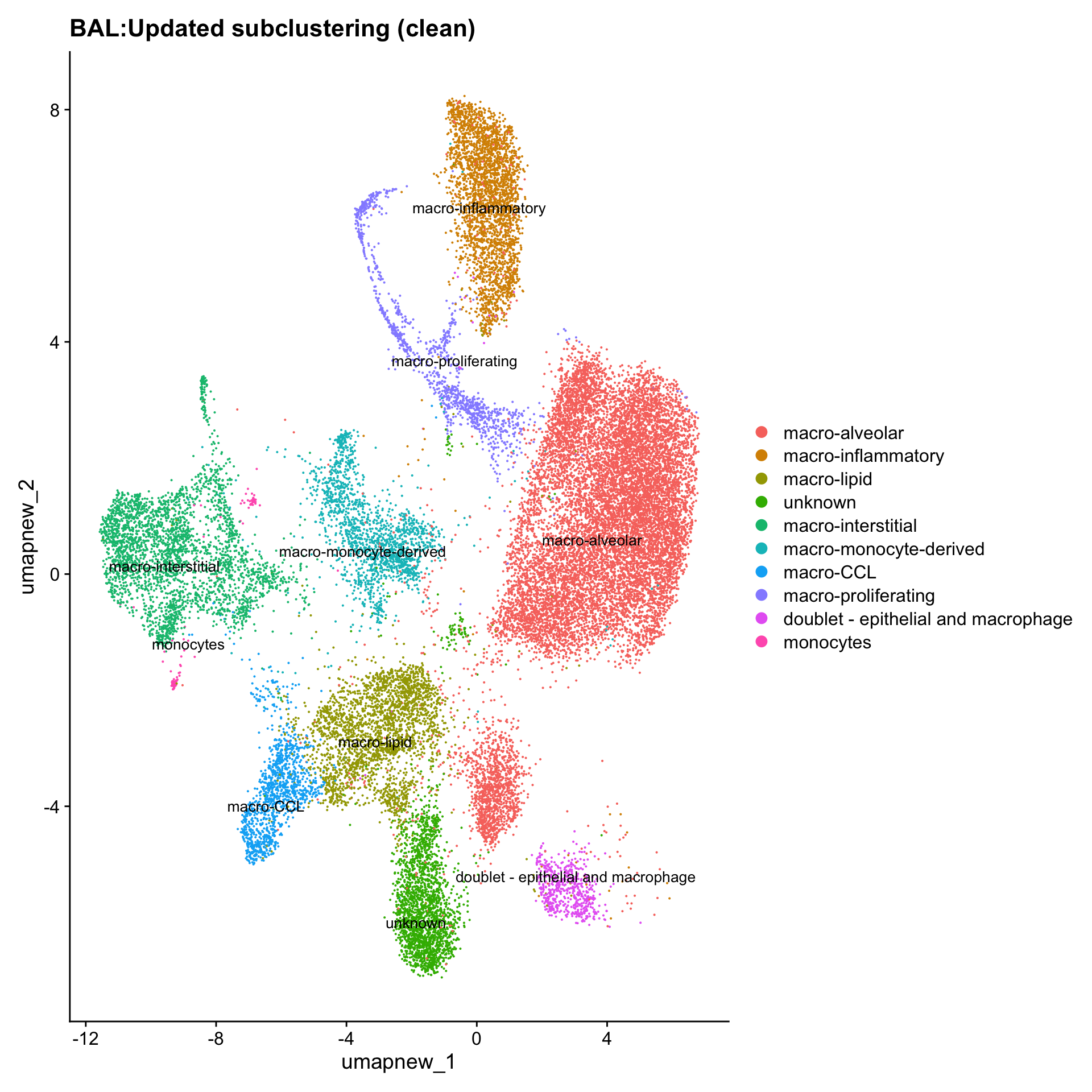

paed_clean <- paed_clean %>%
NormalizeData() %>%
FindVariableFeatures() %>%
ScaleData() %>%
RunPCA()

Normalizing layer: counts

Finding variable features for layer counts

Centering and scaling data matrix

Warning: Different features in new layer data than already exists for
scale.data

PC_ 1 
Positive:  CD52, FABP4, MRC1, FBP1, MCEMP1, LTA4H, CRIP1, LPL, MSR1, ABCG1 
       PECAM1, CYP27A1, GPNMB, PPARG, CD9, GPD1, PCOLCE2, IGFBP2, ANXA1, SCD 
       LYZ, MME, ANXA2, AMIGO2, LGALS3, C8B, EVL, TSPAN3, PDLIM1, GCHFR 
Negative:  SOCS3, IER3, SERPINB9, SOD2, NINJ1, ZFP36, SPHK1, MARCKS, IL4I1, GPR132 
       LILRB2, PFKFB3, NR4A1, C15orf48, IDO1, VEGFA, CCL3, NFKBIA, JUNB, ICAM1 
       STAB1, DUSP1, PIM3, SAT1, NR4A3, TNFRSF1B, TIMP1, HAPLN3, ATF3, CD300E 
PC_ 2 
Positive:  TYMS, MKI67, KIFC1, TOP2A, CENPM, HIST1H1B, RRM2, BIRC5, PCLAF, TPX2 
       CDK1, SPC24, FOXM1, MYBL2, TK1, ANLN, CDCA5, CDT1, UHRF1, ASF1B 
       PRC1, CEP55, AURKB, NCAPG, NDC80, TCF19, GTSE1, CIT, DTL, HJURP 
Negative:  GPD1, C5AR1, MSR1, CD9, TGM2, TFRC, GSN, TYMP, AQP3, ABCG1 
       PCOLCE2, MRC1, EVL, CYP27A1, MCEMP1, FTL, HMOX1, SLC19A3, INHBA, ADGRE3 
       GLRX, RGCC, FCGR3A, ACE, CFD, HBEGF, SQSTM1, CACNB3, TMEM273, LTA4H 
PC_ 3 
Positive:  THBS1, FGL2, TMEM273, CISH, PLAC8, MCEMP1, ISG15, MRC1, HP, PLEKHO1 
       NFE2, PDGFD, IGF1, ADGRE3, CD101, TNFSF10, CD1D, IFI6, IL3RA, AWAT2 
       CD69, ITGAM, ECSCR, FGF10, MS4A6A, IFITM3, MYB, MEFV, PTGER3, AQP3 
Negative:  CSTB, CTSL, TFRC, SCD, LIPA, CXCL3, NR1H3, ABCA1, GPNMB, CD83 
       CD36, APOC1, CXCL2, FTL, AQP9, PLPP3, RMDN3, NRP2, CCL20, LGALS3 
       GCHFR, BCL2A1, ACSL1, LGALS1, CTSB, CCL18, IL1A, PHLDA1, MACC1, SDCBP 
PC_ 4 
Positive:  MS4A6A, GLIPR1, TPM4, CYBB, FPR3, CMTM6, EIF1, CLIC4, CD47, AHR 
       TMEM176B, TMEM123, TMEM176A, SNX2, EVI2B, IFNGR1, RNF13, DEFB1, DNAJA1, MPEG1 
       STT3B, FAM49B, LAMP2, ANXA2, HACD4, EIF4G2, TRAM1, SPPL2A, SNX3, SGMS2 
Negative:  CFD, JUN, SQSTM1, NUPR1, TAGLN, CYP27A1, APOE, TNFAIP2, CCL20, PLAUR 
       TNF, IL1A, TGM2, BCAR1, G0S2, CXCL8, PPP1R15A, CD82, CD83, GPD1 
       GSN, CCL3, CCL4, SDC4, PKD2L1, INHBA, FGR, CD276, BTG2, CXCL2 
PC_ 5 
Positive:  FPR3, EMP1, RASSF2, LMNA, CLEC10A, EMP3, CLEC5A, A2M, RNASE1, CXCR4 
       LGALS1, CST7, ANXA6, BCAT1, F13A1, MYADM, SNCA, ADAM8, PAPSS2, PMP22 
       NRP2, RNASE6, GPAT3, CORO1A, S100A10, ARL4C, ARHGEF40, GPR183, CCR7, CRIP1 
Negative:  CXCL10, APOBEC3A, S100A9, ISG15, CCL8, GBP1, CXCL11, IFIT2, ISG20, IDO1 
       GLUL, GBP5, MX1, IFI6, ACOD1, LILRA5, IFIT3, RSAD2, SERPING1, WARS 
       CD38, GCH1, C8B, IL1RN, GBP2, CALHM6, IL1B, PCOLCE2, LILRB1, TNFSF10 

paed_clean <- RunUMAP(paed_clean, dims = 1:30, reduction = "pca", reduction.name = "umap.clean")

17:10:19 UMAP embedding parameters a = 0.9922 b = 1.112

Found more than one class "dist" in cache; using the first, from namespace 'spam'

Also defined by 'BiocGenerics'

17:10:19 Read 29638 rows and found 30 numeric columns

17:10:19 Using Annoy for neighbor search, n_neighbors = 30

Found more than one class "dist" in cache; using the first, from namespace 'spam'

Also defined by 'BiocGenerics'

17:10:20 Building Annoy index with metric = cosine, n_trees = 50

0%   10   20   30   40   50   60   70   80   90   100%

[----|----|----|----|----|----|----|----|----|----|

**************************************************|
17:10:21 Writing NN index file to temp file /var/folders/q8/kw1r78g12qn793xm7g0zvk94x2bh70/T//RtmpKldB7O/file267c7f876a0d
17:10:21 Searching Annoy index using 1 thread, search_k = 3000
17:10:26 Annoy recall = 100%
17:10:27 Commencing smooth kNN distance calibration using 1 thread with target n_neighbors = 30
17:10:28 Initializing from normalized Laplacian + noise (using RSpectra)
17:10:28 Commencing optimization for 200 epochs, with 1283702 positive edges
17:10:37 Optimization finished

DimPlot(paed_clean, reduction = "umap.clean", group.by = "cell_labels_v2",raster = FALSE, repel = TRUE, label = TRUE, label.size = 4.5) + ggtitle(paste0(tissue, ": Updated subclustering (clean)"))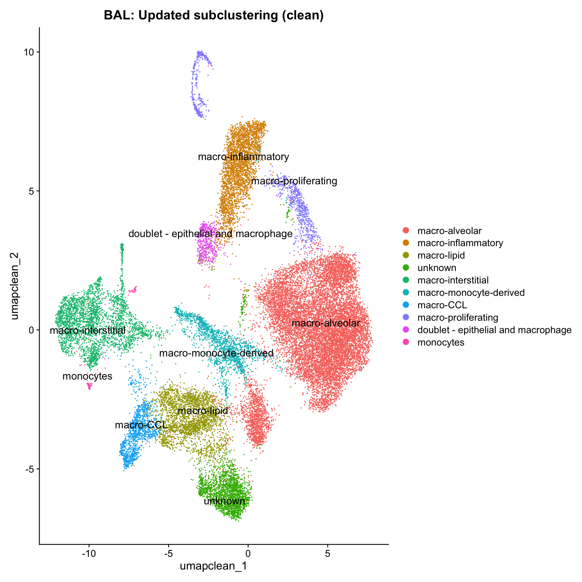

Past versions of unnamed-chunk-29-1.png

Version	Author	Date
0af5a78	Gunjan Dixit	2024-07-30

Reclustering Tcell polulation

This includes CD4 T cell, CD8 T cell, NK cell, NK-T cell, proliferating or cycling T/NK cell.

The marker genes for this reclustering can be found

idx <- which(Idents(seu_obj) %in% c("CD4 T cells", "CD8 T cells", "NK-T cells", "proliferating T/NK", "cycling T cells"))
paed_sub <- seu_obj[,idx]
mito_genes <- grep("^MT-", rownames(paed_sub), value = TRUE)
paed_sub <- subset(paed_sub, features = setdiff(rownames(paed_sub), mito_genes))
paed_sub

An object of class Seurat 
17518 features across 4877 samples within 1 assay 
Active assay: RNA (17518 features, 1990 variable features)
 3 layers present: counts, data, scale.data
 3 dimensional reductions calculated: pca, umap, umap.unintegrated

paed_sub <- paed_sub %>%
  NormalizeData() %>%
  FindVariableFeatures() %>%
  ScaleData() %>%
  RunPCA() 
  
paed_sub <- RunUMAP(paed_sub, dims = 1:30, reduction = "pca", reduction.name = "umap.new")

meta_data_columns <- colnames(paed_sub@meta.data)
columns_to_remove <- grep("^RNA_snn_res", meta_data_columns, value = TRUE)
paed_sub@meta.data <- paed_sub@meta.data[, !(colnames(paed_sub@meta.data) %in% columns_to_remove)]


resolutions <- seq(0.1, 1, by = 0.1)
paed_sub <- FindNeighbors(paed_sub, reduction = "pca", dims = 1:30)
paed_sub <- FindClusters(paed_sub, resolution = resolutions, algorithm = 3)

Modularity Optimizer version 1.3.0 by Ludo Waltman and Nees Jan van Eck

Number of nodes: 4877
Number of edges: 185348

Running smart local moving algorithm...
Maximum modularity in 10 random starts: 0.9386
Number of communities: 5
Elapsed time: 2 seconds
Modularity Optimizer version 1.3.0 by Ludo Waltman and Nees Jan van Eck

Number of nodes: 4877
Number of edges: 185348

Running smart local moving algorithm...
Maximum modularity in 10 random starts: 0.9134
Number of communities: 8
Elapsed time: 2 seconds
Modularity Optimizer version 1.3.0 by Ludo Waltman and Nees Jan van Eck

Number of nodes: 4877
Number of edges: 185348

Running smart local moving algorithm...
Maximum modularity in 10 random starts: 0.8944
Number of communities: 10
Elapsed time: 1 seconds
Modularity Optimizer version 1.3.0 by Ludo Waltman and Nees Jan van Eck

Number of nodes: 4877
Number of edges: 185348

Running smart local moving algorithm...
Maximum modularity in 10 random starts: 0.8777
Number of communities: 12
Elapsed time: 2 seconds
Modularity Optimizer version 1.3.0 by Ludo Waltman and Nees Jan van Eck

Number of nodes: 4877
Number of edges: 185348

Running smart local moving algorithm...
Maximum modularity in 10 random starts: 0.8625
Number of communities: 13
Elapsed time: 1 seconds
Modularity Optimizer version 1.3.0 by Ludo Waltman and Nees Jan van Eck

Number of nodes: 4877
Number of edges: 185348

Running smart local moving algorithm...
Maximum modularity in 10 random starts: 0.8499
Number of communities: 13
Elapsed time: 1 seconds
Modularity Optimizer version 1.3.0 by Ludo Waltman and Nees Jan van Eck

Number of nodes: 4877
Number of edges: 185348

Running smart local moving algorithm...
Maximum modularity in 10 random starts: 0.8376
Number of communities: 14
Elapsed time: 1 seconds
Modularity Optimizer version 1.3.0 by Ludo Waltman and Nees Jan van Eck

Number of nodes: 4877
Number of edges: 185348

Running smart local moving algorithm...
Maximum modularity in 10 random starts: 0.8279
Number of communities: 16
Elapsed time: 1 seconds
Modularity Optimizer version 1.3.0 by Ludo Waltman and Nees Jan van Eck

Number of nodes: 4877
Number of edges: 185348

Running smart local moving algorithm...
Maximum modularity in 10 random starts: 0.8186
Number of communities: 16
Elapsed time: 1 seconds
Modularity Optimizer version 1.3.0 by Ludo Waltman and Nees Jan van Eck

Number of nodes: 4877
Number of edges: 185348

Running smart local moving algorithm...
Maximum modularity in 10 random starts: 0.8096
Number of communities: 17
Elapsed time: 1 seconds

DimHeatmap(paed_sub, dims = 1:10, cells = 500, balanced = TRUE)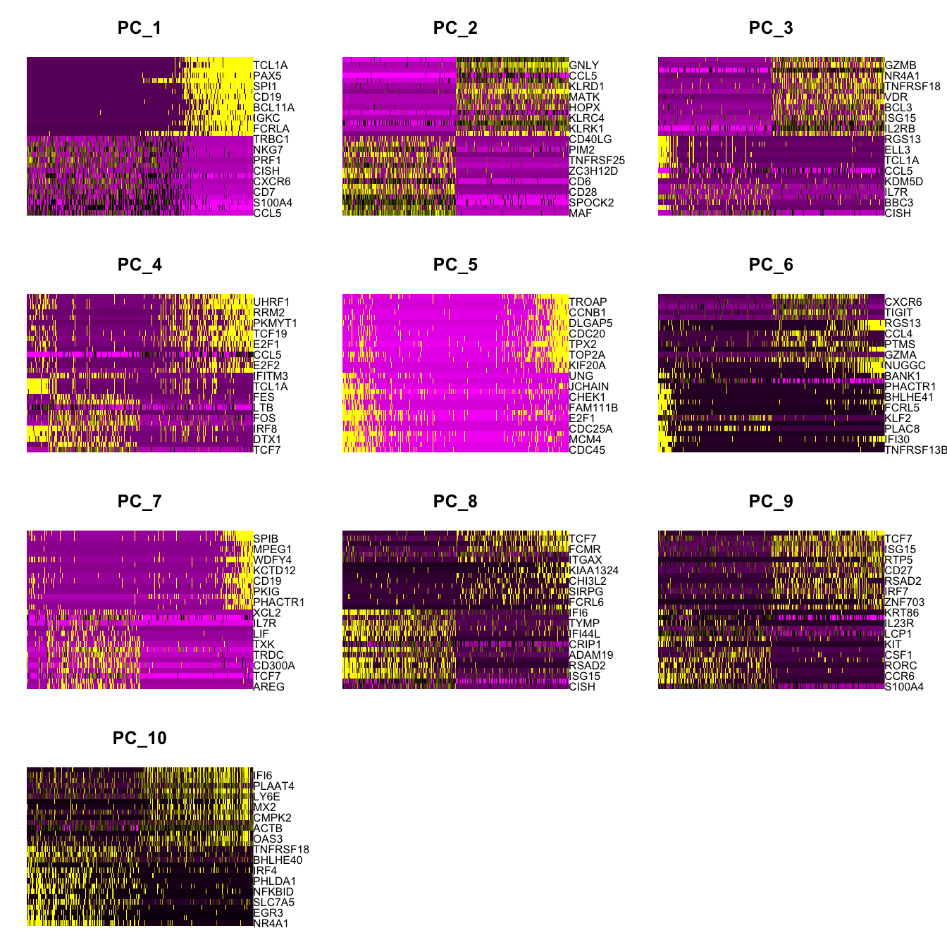

Past versions of unnamed-chunk-31-1.png

Version	Author	Date
c20f60f	Gunjan Dixit	2024-07-08

clustree(paed_sub, prefix = "RNA_snn_res.")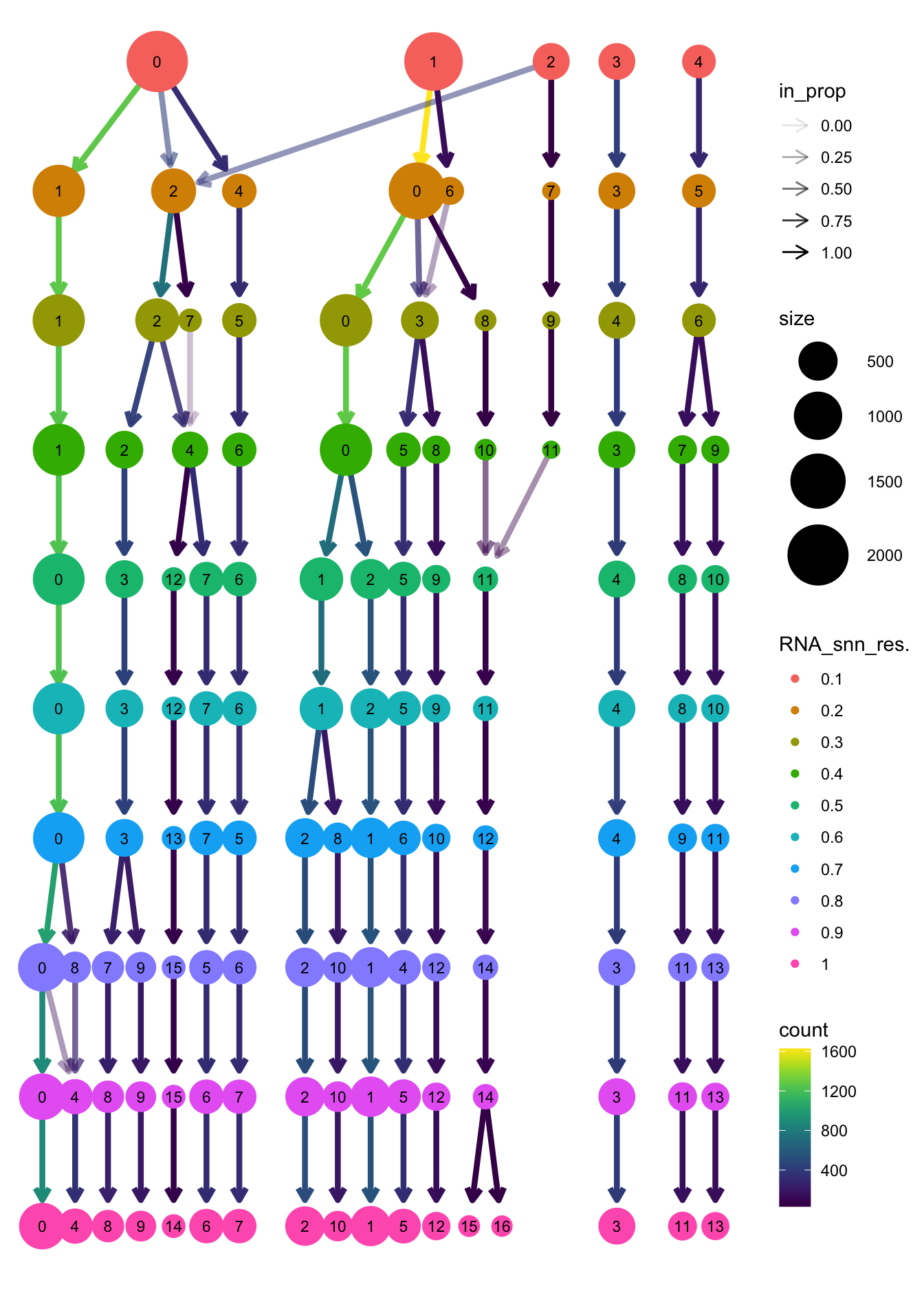

opt_res <- "RNA_snn_res.0.4"  
n <- nlevels(paed_sub$RNA_snn_res.0.4)
paed_sub$RNA_snn_res.0.4 <- factor(paed_sub$RNA_snn_res.0.4, levels = seq(0,n-1))
paed_sub$seurat_clusters <- NULL
paed_sub$cluster <- paed_sub$RNA_snn_res.0.4
Idents(paed_sub) <- paed_sub$cluster

paed_sub.markers <- FindAllMarkers(paed_sub, only.pos = TRUE, min.pct = 0.25, logfc.threshold = 0.25)

Calculating cluster 0

Calculating cluster 1

Calculating cluster 2

Calculating cluster 3

Calculating cluster 4

Calculating cluster 5

Calculating cluster 6

Calculating cluster 7

Calculating cluster 8

Calculating cluster 9

Calculating cluster 10

Calculating cluster 11

paed_sub.markers %>%
    group_by(cluster) %>% unique() %>% 
    top_n(n = 5, wt = avg_log2FC) -> top5

paed_sub.markers %>%
    group_by(cluster) %>% 
    slice_head(n=1) %>% 
    pull(gene) -> best.wilcox.gene.per.cluster

best.wilcox.gene.per.cluster

 [1] "CD4"    "CCL5"   "TCF7"   "NMUR1"  "AREG"   "MAF"    "GZMB"   "CD79A" 
 [9] "CXCR5"  "TYMS"   "SCART1" "CX3CR1"

Feature plot shows the expression of top marker genes per cluster.

FeaturePlot(paed_sub,features=best.wilcox.gene.per.cluster, reduction = 'umap.new', raster = FALSE, ncol = 2, label = TRUE)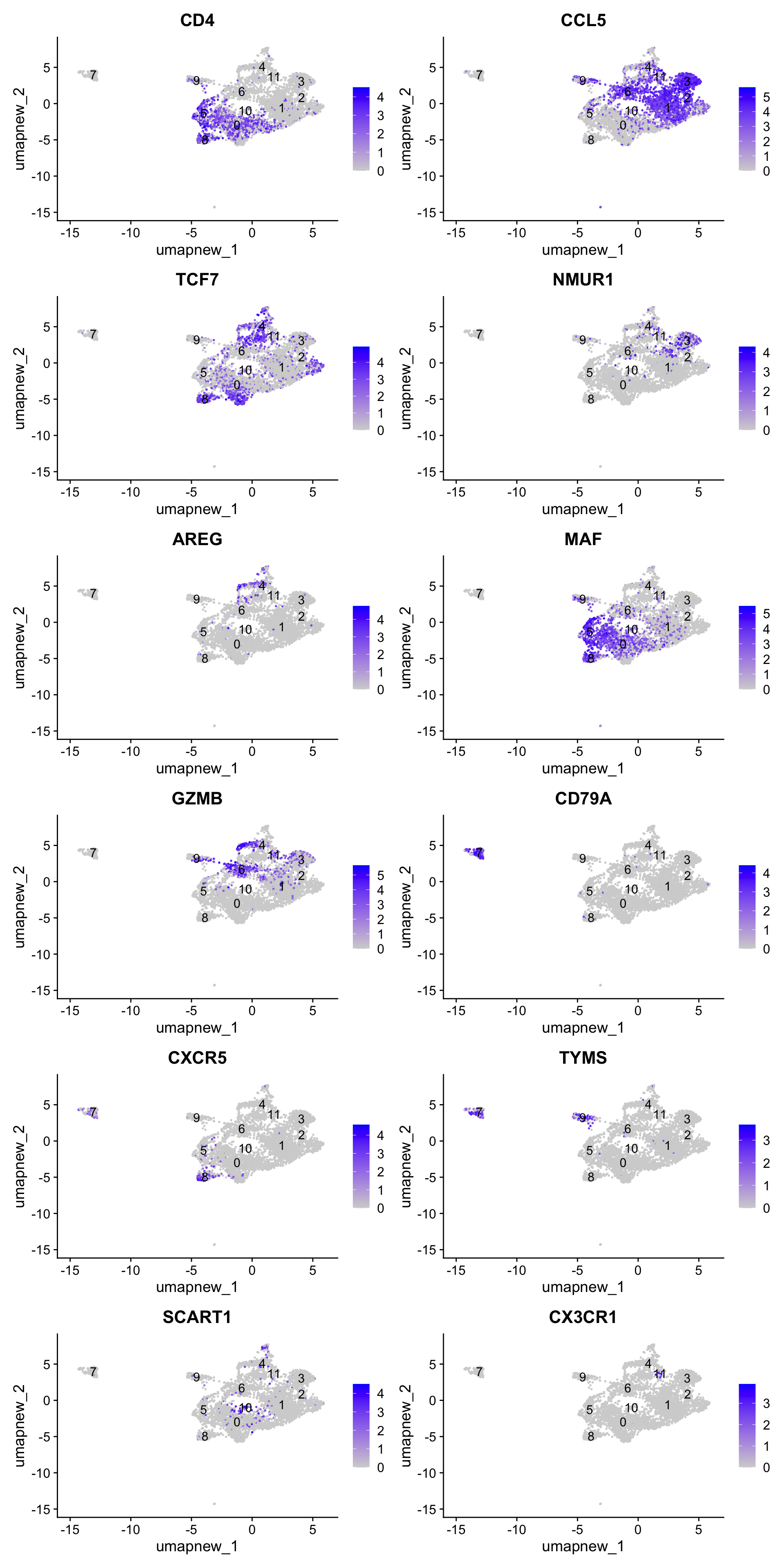

Top 10 marker genes from Seurat

## Seurat top markers
top10 <- paed_sub.markers %>%
    group_by(cluster) %>%
    top_n(n = 10, wt = avg_log2FC) %>%
    ungroup() %>%
    distinct(gene, .keep_all = TRUE) %>%
    arrange(cluster, desc(avg_log2FC))

cluster_colors <- paletteer::paletteer_d("pals::glasbey")[factor(top10$cluster)]

DotPlot(paed_sub,    
        features = unique(top10$gene),
        group.by = opt_res,
        cols = c("azure1", "blueviolet"),
        dot.scale = 3, assay = "RNA") +
    RotatedAxis() +
    FontSize(y.text = 8, x.text = 12) +
    labs(y = element_blank(), x = element_blank()) +
    coord_flip() +
    theme(axis.text.y = element_text(color = cluster_colors)) +
    ggtitle("Top 10 marker genes per cluster (Seurat)")

Warning: Vectorized input to `element_text()` is not officially supported.
ℹ Results may be unexpected or may change in future versions of ggplot2.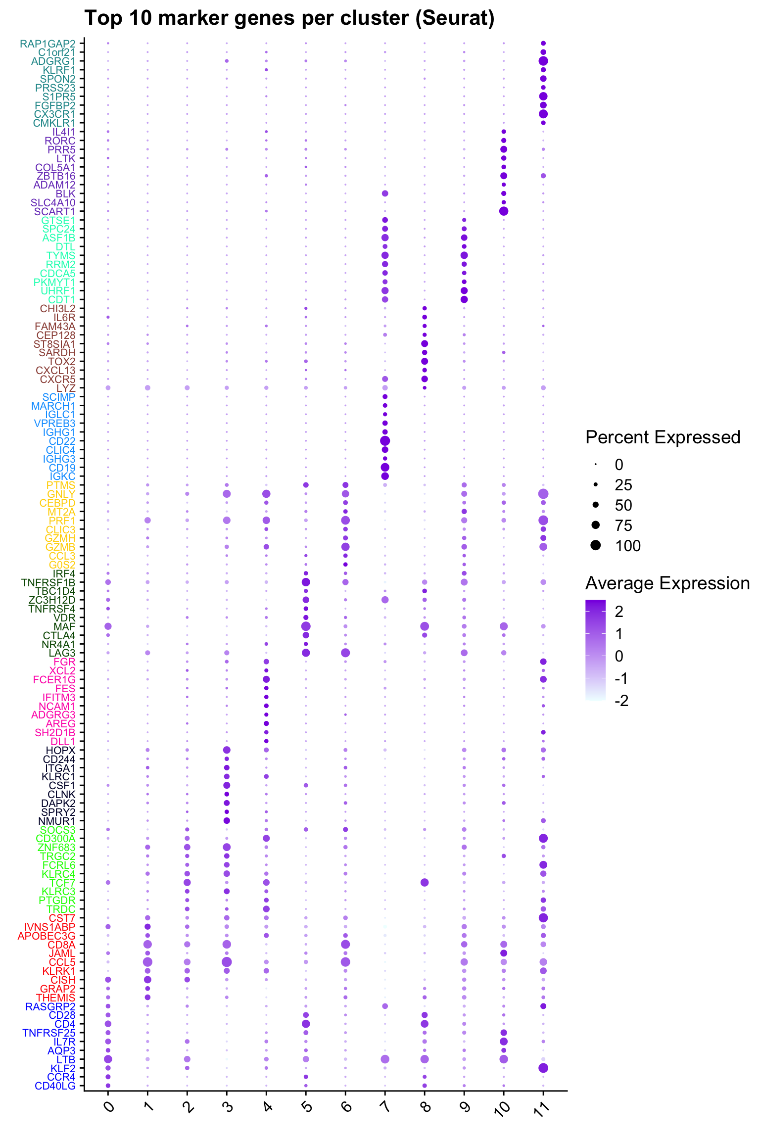

Past versions of unnamed-chunk-36-1.png

Version	Author	Date
0af5a78	Gunjan Dixit	2024-07-30

out_markers <- here("output",
            "CSV", 
            paste(tissue,"_Marker_genes_Reclustered_Tcell_population.",opt_res, sep = ""))

dir.create(out_markers, recursive = TRUE, showWarnings = FALSE)

for (cl in unique(paed_sub.markers$cluster)) {
  cluster_data <- paed_sub.markers %>% dplyr::filter(cluster == cl)
  file_name <- here(out_markers, paste0("G000231_Neeland_",tissue, "_cluster_", cl, ".csv"))
  write.csv(cluster_data, file = file_name)
}

Update T cell subclustering labels

cell_labels <- readxl::read_excel(here("data/Cell_labels_Mel_v2/earlyAIR_NB_BB_BAL_T-NK_annotations_16.07.24.xlsx"), sheet = "BAL")
new_cluster_names <- cell_labels %>% 
  dplyr::select(cluster, annotation) %>% 
  deframe()

paed_sub <- RenameIdents(paed_sub, new_cluster_names)
paed_sub@meta.data$cell_labels_v2 <- Idents(paed_sub)

DimPlot(paed_sub, reduction = "umap.new", raster = FALSE, repel = TRUE, label = TRUE, label.size = 3.5) + ggtitle(paste0(tissue, ": UMAP with Updated cell types"))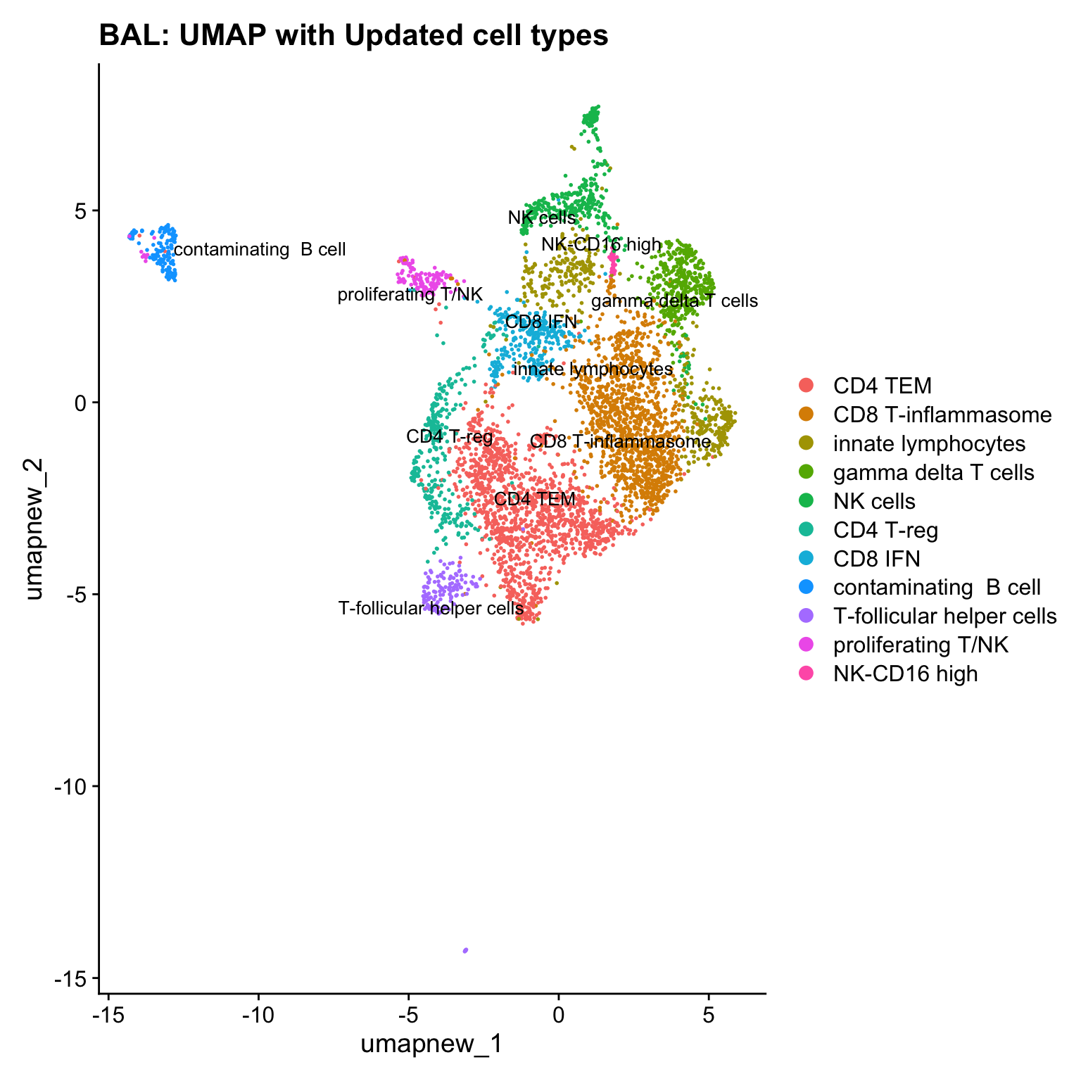

Past versions of unnamed-chunk-38-1.png

Version	Author	Date
0af5a78	Gunjan Dixit	2024-07-30

Excluding contaminating labels

idx <- which(grepl("^contaminating", Idents(paed_sub)))
paed_clean <- paed_sub[, -idx]
DimPlot(paed_clean, reduction = "umap.new", raster = FALSE, repel = TRUE, label = TRUE, label.size = 3.5) + ggtitle(paste0(tissue, ": Updated subclustering (clean)"))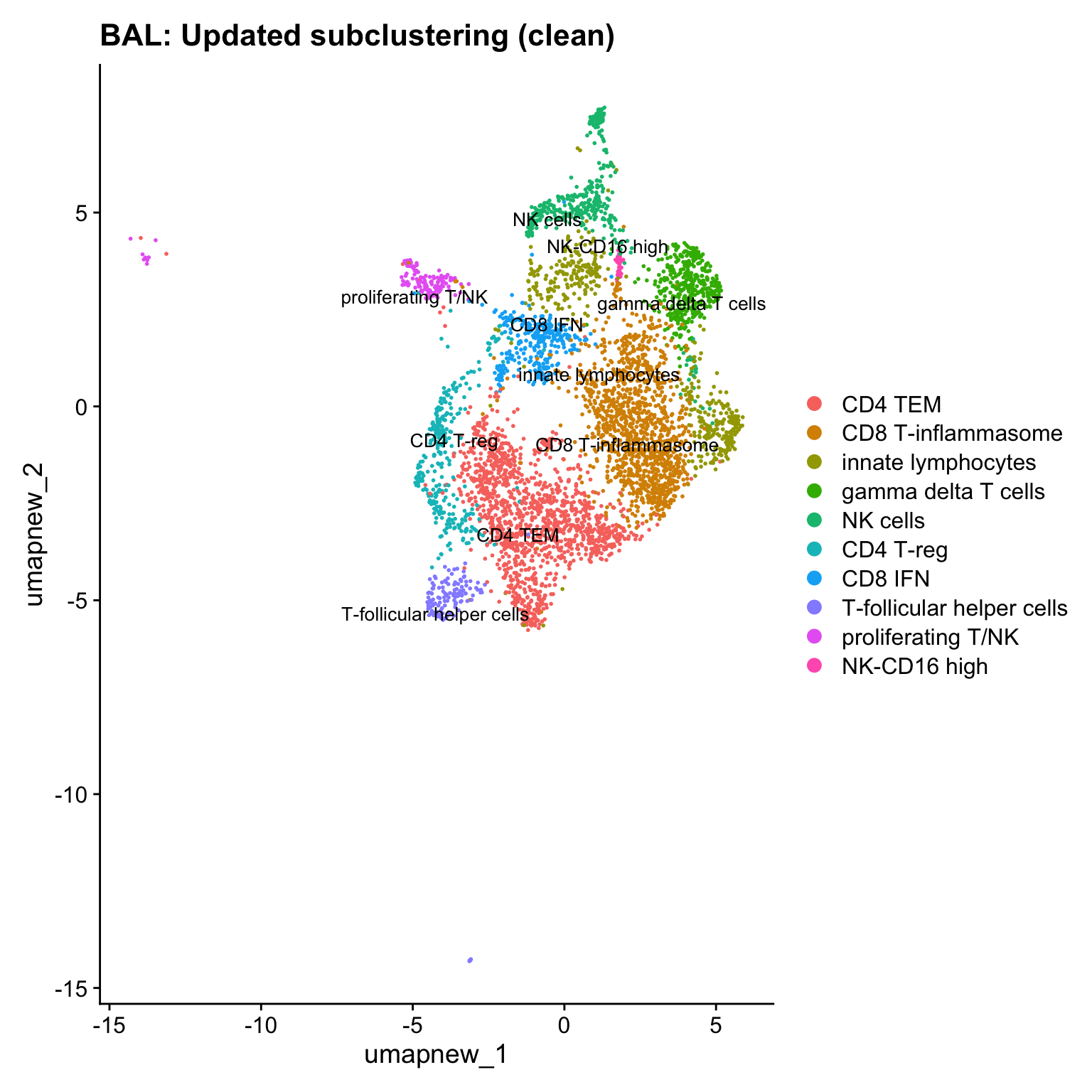

paed_clean <- paed_clean %>%
NormalizeData() %>%
FindVariableFeatures() %>%
ScaleData() %>%
RunPCA()

Normalizing layer: counts

Finding variable features for layer counts

Centering and scaling data matrix

Warning: Different features in new layer data than already exists for
scale.data

PC_ 1 
Positive:  IL7R, TCF7, CISH, PTGDR, KLRK1, TSC22D3, KLRC3, AOAH, TRGC2, FCRL6 
       OBSCN, TRGC1, PLXDC1, KLRC4, CCDC141, SCML4, NMUR1, SPRY2, PTGER2, TRDC 
       TC2N, NELL2, FCGBP, ADAMTS10, ABCB1, LEF1, TRGJP2, TTN, GCSAM, PIK3R1 
Negative:  TYMS, CDT1, UHRF1, RRM2, MKI67, HIST1H1B, KIFC1, ASF1B, MYBL2, AURKB 
       ZWINT, TOP2A, TK1, PKMYT1, CDCA5, SPC24, DTL, E2F1, FOXM1, BIRC5 
       PCLAF, STMN1, HIST1H2BH, ESPL1, TPX2, NUSAP1, GTSE1, ASPM, CDK1, E2F2 
PC_ 2 
Positive:  MAF, CD4, SPOCK2, LTB, CD28, CCR4, ZC3H12D, CD6, CTLA4, TNFRSF25 
       CD5, TNFRSF4, PIM2, AQP3, PBXIP1, CD40LG, ICOS, COL5A3, TMEM173, CTSH 
       IL7R, CCR6, IL6R, TNFRSF1B, ADAM19, NPDC1, IL2RA, CERK, SLAMF1, TBC1D4 
Negative:  NKG7, CTSW, GNLY, CCL5, PRF1, ZNF683, KLRD1, CD8A, MATK, ITGAX 
       HOPX, KLRC4, CD7, KLRK1, GZMB, NCR1, KLRC3, PIK3AP1, KLRC1, NMUR1 
       RIN3, FCRL6, AOAH, FGR, TRDC, KIR2DL4, GZMA, IL2RB, ITM2C, SPRY2 
PC_ 3 
Positive:  FURIN, DUSP2, SRGN, GZMB, TNFRSF18, NR4A1, IL2RB, FOSL2, GNLY, CD38 
       DDIT4, CD7, VDR, ZFP36, ISG15, BCL3, IFI6, SOCS3, FOS, AREG 
       JUNB, IFITM3, HAPLN3, IRF8, SBNO2, SH2D2A, NR4A2, ISG20, NFKBIA, NR4A3 
Negative:  CISH, VIM, HIST1H1C, ANXA1, RRM2, CRIP1, BBC3, HIST1H1B, GRAP2, PLP2 
       TOP2A, ASPM, TRIB3, MKI67, TYMS, CCL5, HIST1H1D, KIFC1, NCAPG, ANKRD28 
       HIST1H2BH, KDM5D, STMN1, HJURP, FAM111A, CKS1B, TC2N, CDK1, UTY, JAML 
PC_ 4 
Positive:  LAG3, CCL5, CXCR6, CD8A, GZMA, CCR5, IL32, PTMS, TIGIT, CCL4 
       CSF1, TRBC2, GPR25, ITGA1, DUSP4, ABI3, DAPK2, PRDM1, CCL4L2, TNFRSF1B 
       LBH, PLAAT4, PHLDA1, PDCD1, FASLG, CD6, S100A4, JUN, CCL3, GZMH 
Negative:  TCF7, AREG, PLAC8, DLL1, KLF2, CD300A, IL7R, TRDC, NCAM1, IFITM3 
       LTB, SH2D1B, TXK, KIT, FES, TNFRSF18, RIPOR2, ITGAM, PTGDR, SELL 
       LIF, ADGRG3, SLC16A3, XCL2, FGR, IRF8, S1PR1, KLRF1, SORL1, BHLHE40 
PC_ 5 
Positive:  CXCR5, TOX2, TCF7, IGHM, FCMR, POU2AF1, CHI3L2, GNG4, ID3, CD7 
       KIAA1324, SARDH, ITGAX, SIRPG, NMUR1, RTP5, CDK5R1, ZNF703, IL21, ST8SIA1 
       TBC1D4, FCRL6, CXXC5, TSPOAP1, MAGEH1, FAM43A, CXCL13, KCNK5, LTBP3, SPRY2 
Negative:  CISH, VIM, ISG15, ANXA1, CRIP1, RSAD2, OAS3, MX1, CMPK2, ADAM19 
       LGALS1, IFI44L, OAS1, IFI6, IFIT1, MYADM, XAF1, LY6E, TYMP, CCR5 
       PRF1, BHLHE40, GBP1, OAS2, OASL, IFI44, USP18, GZMB, IRF7, APOBEC3G 

paed_clean <- RunUMAP(paed_clean, dims = 1:30, reduction = "pca", reduction.name = "umap.clean")

17:11:23 UMAP embedding parameters a = 0.9922 b = 1.112

Found more than one class "dist" in cache; using the first, from namespace 'spam'

Also defined by 'BiocGenerics'

17:11:23 Read 4724 rows and found 30 numeric columns

17:11:23 Using Annoy for neighbor search, n_neighbors = 30

Found more than one class "dist" in cache; using the first, from namespace 'spam'

Also defined by 'BiocGenerics'

17:11:23 Building Annoy index with metric = cosine, n_trees = 50

0%   10   20   30   40   50   60   70   80   90   100%

[----|----|----|----|----|----|----|----|----|----|

**************************************************|
17:11:23 Writing NN index file to temp file /var/folders/q8/kw1r78g12qn793xm7g0zvk94x2bh70/T//RtmpKldB7O/file267c1634c7cd
17:11:23 Searching Annoy index using 1 thread, search_k = 3000
17:11:24 Annoy recall = 100%
17:11:24 Commencing smooth kNN distance calibration using 1 thread with target n_neighbors = 30
17:11:25 Initializing from normalized Laplacian + noise (using RSpectra)
17:11:25 Commencing optimization for 500 epochs, with 194062 positive edges
17:11:29 Optimization finished

DimPlot(paed_clean, reduction = "umap.clean", group.by = "cell_labels_v2",raster = FALSE, repel = TRUE, label = TRUE, label.size = 4.5) + ggtitle(paste0(tissue, ": Updated subclustering (clean)"))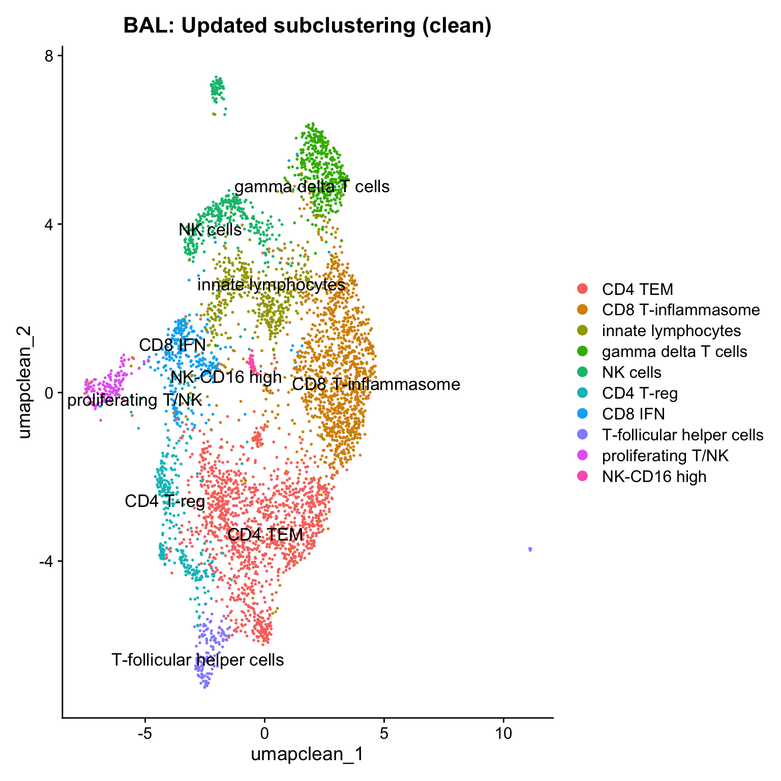

Session Info

sessioninfo::session_info()

─ Session info ───────────────────────────────────────────────────────────────
 setting  value
 version  R version 4.3.2 (2023-10-31)
 os       macOS Sonoma 14.5
 system   aarch64, darwin20
 ui       X11
 language (EN)
 collate  en_US.UTF-8
 ctype    en_US.UTF-8
 tz       Australia/Melbourne
 date     2024-07-30
 pandoc   3.1.1 @ /Users/dixitgunjan/Desktop/RStudio.app/Contents/Resources/app/quarto/bin/tools/ (via rmarkdown)

─ Packages ───────────────────────────────────────────────────────────────────
 package              * version    date (UTC) lib source
 abind                  1.4-5      2016-07-21 [1] CRAN (R 4.3.0)
 AnnotationDbi        * 1.64.1     2023-11-02 [1] Bioconductor
 backports              1.4.1      2021-12-13 [1] CRAN (R 4.3.0)
 beeswarm               0.4.0      2021-06-01 [1] CRAN (R 4.3.0)
 Biobase              * 2.62.0     2023-10-26 [1] Bioconductor
 BiocGenerics         * 0.48.1     2023-11-02 [1] Bioconductor
 BiocManager            1.30.22    2023-08-08 [1] CRAN (R 4.3.0)
 BiocStyle            * 2.30.0     2023-10-26 [1] Bioconductor
 Biostrings             2.70.2     2024-01-30 [1] Bioconductor 3.18 (R 4.3.2)
 bit                    4.0.5      2022-11-15 [1] CRAN (R 4.3.0)
 bit64                  4.0.5      2020-08-30 [1] CRAN (R 4.3.0)
 bitops                 1.0-7      2021-04-24 [1] CRAN (R 4.3.0)
 blob                   1.2.4      2023-03-17 [1] CRAN (R 4.3.0)
 bslib                  0.6.1      2023-11-28 [1] CRAN (R 4.3.1)
 cachem                 1.0.8      2023-05-01 [1] CRAN (R 4.3.0)
 callr                  3.7.5      2024-02-19 [1] CRAN (R 4.3.1)
 cellranger             1.1.0      2016-07-27 [1] CRAN (R 4.3.0)
 checkmate              2.3.1      2023-12-04 [1] CRAN (R 4.3.1)
 cli                    3.6.2      2023-12-11 [1] CRAN (R 4.3.1)
 cluster                2.1.6      2023-12-01 [1] CRAN (R 4.3.1)
 clustree             * 0.5.1      2023-11-05 [1] CRAN (R 4.3.1)
 codetools              0.2-19     2023-02-01 [1] CRAN (R 4.3.2)
 colorspace             2.1-0      2023-01-23 [1] CRAN (R 4.3.0)
 cowplot                1.1.3      2024-01-22 [1] CRAN (R 4.3.1)
 crayon                 1.5.2      2022-09-29 [1] CRAN (R 4.3.0)
 data.table           * 1.15.0     2024-01-30 [1] CRAN (R 4.3.1)
 DBI                    1.2.2      2024-02-16 [1] CRAN (R 4.3.1)
 DelayedArray           0.28.0     2023-11-06 [1] Bioconductor
 deldir                 2.0-2      2023-11-23 [1] CRAN (R 4.3.1)
 digest                 0.6.34     2024-01-11 [1] CRAN (R 4.3.1)
 dotCall64              1.1-1      2023-11-28 [1] CRAN (R 4.3.1)
 dplyr                * 1.1.4      2023-11-17 [1] CRAN (R 4.3.1)
 edgeR                * 4.0.16     2024-02-20 [1] Bioconductor 3.18 (R 4.3.2)
 ellipsis               0.3.2      2021-04-29 [1] CRAN (R 4.3.0)
 evaluate               0.23       2023-11-01 [1] CRAN (R 4.3.1)
 fansi                  1.0.6      2023-12-08 [1] CRAN (R 4.3.1)
 farver                 2.1.1      2022-07-06 [1] CRAN (R 4.3.0)
 fastDummies            1.7.3      2023-07-06 [1] CRAN (R 4.3.0)
 fastmap                1.1.1      2023-02-24 [1] CRAN (R 4.3.0)
 fitdistrplus           1.1-11     2023-04-25 [1] CRAN (R 4.3.0)
 forcats              * 1.0.0      2023-01-29 [1] CRAN (R 4.3.0)
 fs                     1.6.3      2023-07-20 [1] CRAN (R 4.3.0)
 future                 1.33.1     2023-12-22 [1] CRAN (R 4.3.1)
 future.apply           1.11.1     2023-12-21 [1] CRAN (R 4.3.1)
 generics               0.1.3      2022-07-05 [1] CRAN (R 4.3.0)
 GenomeInfoDb           1.38.6     2024-02-10 [1] Bioconductor 3.18 (R 4.3.2)
 GenomeInfoDbData       1.2.11     2024-02-27 [1] Bioconductor
 GenomicRanges          1.54.1     2023-10-30 [1] Bioconductor
 getPass                0.2-4      2023-12-10 [1] CRAN (R 4.3.1)
 ggbeeswarm             0.7.2      2023-04-29 [1] CRAN (R 4.3.0)
 ggforce                0.4.2      2024-02-19 [1] CRAN (R 4.3.1)
 ggplot2              * 3.5.0      2024-02-23 [1] CRAN (R 4.3.1)
 ggraph               * 2.1.0      2022-10-09 [1] CRAN (R 4.3.0)
 ggrastr                1.0.2      2023-06-01 [1] CRAN (R 4.3.0)
 ggrepel                0.9.5      2024-01-10 [1] CRAN (R 4.3.1)
 ggridges               0.5.6      2024-01-23 [1] CRAN (R 4.3.1)
 git2r                  0.33.0     2023-11-26 [1] CRAN (R 4.3.1)
 globals                0.16.2     2022-11-21 [1] CRAN (R 4.3.0)
 glue                 * 1.7.0      2024-01-09 [1] CRAN (R 4.3.1)
 goftest                1.2-3      2021-10-07 [1] CRAN (R 4.3.0)
 graphlayouts           1.1.0      2024-01-19 [1] CRAN (R 4.3.1)
 gridExtra              2.3        2017-09-09 [1] CRAN (R 4.3.0)
 gtable                 0.3.4      2023-08-21 [1] CRAN (R 4.3.0)
 here                 * 1.0.1      2020-12-13 [1] CRAN (R 4.3.0)
 highr                  0.10       2022-12-22 [1] CRAN (R 4.3.0)
 hms                    1.1.3      2023-03-21 [1] CRAN (R 4.3.0)
 htmltools              0.5.7      2023-11-03 [1] CRAN (R 4.3.1)
 htmlwidgets            1.6.4      2023-12-06 [1] CRAN (R 4.3.1)
 httpuv                 1.6.14     2024-01-26 [1] CRAN (R 4.3.1)
 httr                   1.4.7      2023-08-15 [1] CRAN (R 4.3.0)
 ica                    1.0-3      2022-07-08 [1] CRAN (R 4.3.0)
 igraph                 2.0.2      2024-02-17 [1] CRAN (R 4.3.1)
 IRanges              * 2.36.0     2023-10-26 [1] Bioconductor
 irlba                  2.3.5.1    2022-10-03 [1] CRAN (R 4.3.2)
 jquerylib              0.1.4      2021-04-26 [1] CRAN (R 4.3.0)
 jsonlite               1.8.8      2023-12-04 [1] CRAN (R 4.3.1)
 kableExtra           * 1.4.0      2024-01-24 [1] CRAN (R 4.3.1)
 KEGGREST               1.42.0     2023-10-26 [1] Bioconductor
 KernSmooth             2.23-22    2023-07-10 [1] CRAN (R 4.3.2)
 knitr                  1.45       2023-10-30 [1] CRAN (R 4.3.1)
 labeling               0.4.3      2023-08-29 [1] CRAN (R 4.3.0)
 later                  1.3.2      2023-12-06 [1] CRAN (R 4.3.1)
 lattice                0.22-5     2023-10-24 [1] CRAN (R 4.3.1)
 lazyeval               0.2.2      2019-03-15 [1] CRAN (R 4.3.0)
 leiden                 0.4.3.1    2023-11-17 [1] CRAN (R 4.3.1)
 lifecycle              1.0.4      2023-11-07 [1] CRAN (R 4.3.1)
 limma                * 3.58.1     2023-11-02 [1] Bioconductor
 listenv                0.9.1      2024-01-29 [1] CRAN (R 4.3.1)
 lmtest                 0.9-40     2022-03-21 [1] CRAN (R 4.3.0)
 locfit                 1.5-9.8    2023-06-11 [1] CRAN (R 4.3.0)
 lubridate            * 1.9.3      2023-09-27 [1] CRAN (R 4.3.1)
 magrittr               2.0.3      2022-03-30 [1] CRAN (R 4.3.0)
 MASS                   7.3-60.0.1 2024-01-13 [1] CRAN (R 4.3.1)
 Matrix                 1.6-5      2024-01-11 [1] CRAN (R 4.3.1)
 MatrixGenerics         1.14.0     2023-10-26 [1] Bioconductor
 matrixStats            1.2.0      2023-12-11 [1] CRAN (R 4.3.1)
 memoise                2.0.1      2021-11-26 [1] CRAN (R 4.3.0)
 mime                   0.12       2021-09-28 [1] CRAN (R 4.3.0)
 miniUI                 0.1.1.1    2018-05-18 [1] CRAN (R 4.3.0)
 munsell                0.5.0      2018-06-12 [1] CRAN (R 4.3.0)
 nlme                   3.1-164    2023-11-27 [1] CRAN (R 4.3.1)
 org.Hs.eg.db         * 3.18.0     2024-02-27 [1] Bioconductor
 paletteer              1.6.0      2024-01-21 [1] CRAN (R 4.3.1)
 parallelly             1.37.0     2024-02-14 [1] CRAN (R 4.3.1)
 patchwork            * 1.2.0      2024-01-08 [1] CRAN (R 4.3.1)
 pbapply                1.7-2      2023-06-27 [1] CRAN (R 4.3.0)
 pillar                 1.9.0      2023-03-22 [1] CRAN (R 4.3.0)
 pkgconfig              2.0.3      2019-09-22 [1] CRAN (R 4.3.0)
 plotly                 4.10.4     2024-01-13 [1] CRAN (R 4.3.1)
 plyr                   1.8.9      2023-10-02 [1] CRAN (R 4.3.1)
 png                    0.1-8      2022-11-29 [1] CRAN (R 4.3.0)
 polyclip               1.10-6     2023-09-27 [1] CRAN (R 4.3.1)
 presto                 1.0.0      2024-02-27 [1] Github (immunogenomics/presto@31dc97f)
 prismatic              1.1.1      2022-08-15 [1] CRAN (R 4.3.0)
 processx               3.8.3      2023-12-10 [1] CRAN (R 4.3.1)
 progressr              0.14.0     2023-08-10 [1] CRAN (R 4.3.0)
 promises               1.2.1      2023-08-10 [1] CRAN (R 4.3.0)
 ps                     1.7.6      2024-01-18 [1] CRAN (R 4.3.1)
 purrr                * 1.0.2      2023-08-10 [1] CRAN (R 4.3.0)
 R6                     2.5.1      2021-08-19 [1] CRAN (R 4.3.0)
 RANN                   2.6.1      2019-01-08 [1] CRAN (R 4.3.0)
 RColorBrewer         * 1.1-3      2022-04-03 [1] CRAN (R 4.3.0)
 Rcpp                   1.0.12     2024-01-09 [1] CRAN (R 4.3.1)
 RcppAnnoy              0.0.22     2024-01-23 [1] CRAN (R 4.3.1)
 RcppHNSW               0.6.0      2024-02-04 [1] CRAN (R 4.3.1)
 RCurl                  1.98-1.14  2024-01-09 [1] CRAN (R 4.3.1)
 readr                * 2.1.5      2024-01-10 [1] CRAN (R 4.3.1)
 readxl               * 1.4.3      2023-07-06 [1] CRAN (R 4.3.0)
 rematch2               2.1.2      2020-05-01 [1] CRAN (R 4.3.0)
 reshape2               1.4.4      2020-04-09 [1] CRAN (R 4.3.0)
 reticulate             1.35.0     2024-01-31 [1] CRAN (R 4.3.1)
 rlang                  1.1.3      2024-01-10 [1] CRAN (R 4.3.1)
 rmarkdown              2.25       2023-09-18 [1] CRAN (R 4.3.1)
 ROCR                   1.0-11     2020-05-02 [1] CRAN (R 4.3.0)
 rprojroot              2.0.4      2023-11-05 [1] CRAN (R 4.3.1)
 RSpectra               0.16-1     2022-04-24 [1] CRAN (R 4.3.0)
 RSQLite                2.3.5      2024-01-21 [1] CRAN (R 4.3.1)
 rstudioapi             0.15.0     2023-07-07 [1] CRAN (R 4.3.0)
 Rtsne                  0.17       2023-12-07 [1] CRAN (R 4.3.1)
 S4Arrays               1.2.0      2023-10-26 [1] Bioconductor
 S4Vectors            * 0.40.2     2023-11-25 [1] Bioconductor 3.18 (R 4.3.2)
 sass                   0.4.8      2023-12-06 [1] CRAN (R 4.3.1)
 scales                 1.3.0      2023-11-28 [1] CRAN (R 4.3.1)
 scattermore            1.2        2023-06-12 [1] CRAN (R 4.3.0)
 sctransform            0.4.1      2023-10-19 [1] CRAN (R 4.3.1)
 sessioninfo            1.2.2      2021-12-06 [1] CRAN (R 4.3.0)
 Seurat               * 5.0.1.9009 2024-02-28 [1] Github (satijalab/seurat@6a3ef5e)
 SeuratObject         * 5.0.1      2023-11-17 [1] CRAN (R 4.3.1)
 shiny                  1.8.0      2023-11-17 [1] CRAN (R 4.3.1)
 SingleCellExperiment   1.24.0     2023-11-06 [1] Bioconductor
 sp                   * 2.1-3      2024-01-30 [1] CRAN (R 4.3.1)
 spam                   2.10-0     2023-10-23 [1] CRAN (R 4.3.1)
 SparseArray            1.2.4      2024-02-10 [1] Bioconductor 3.18 (R 4.3.2)
 spatstat.data          3.0-4      2024-01-15 [1] CRAN (R 4.3.1)
 spatstat.explore       3.2-6      2024-02-01 [1] CRAN (R 4.3.1)
 spatstat.geom          3.2-8      2024-01-26 [1] CRAN (R 4.3.1)
 spatstat.random        3.2-2      2023-11-29 [1] CRAN (R 4.3.1)
 spatstat.sparse        3.0-3      2023-10-24 [1] CRAN (R 4.3.1)
 spatstat.utils         3.0-4      2023-10-24 [1] CRAN (R 4.3.1)
 speckle              * 1.2.0      2023-10-26 [1] Bioconductor
 statmod                1.5.0      2023-01-06 [1] CRAN (R 4.3.0)
 stringi                1.8.3      2023-12-11 [1] CRAN (R 4.3.1)
 stringr              * 1.5.1      2023-11-14 [1] CRAN (R 4.3.1)
 SummarizedExperiment   1.32.0     2023-11-06 [1] Bioconductor
 survival               3.5-8      2024-02-14 [1] CRAN (R 4.3.1)
 svglite                2.1.3      2023-12-08 [1] CRAN (R 4.3.1)
 systemfonts            1.0.5      2023-10-09 [1] CRAN (R 4.3.1)
 tensor                 1.5        2012-05-05 [1] CRAN (R 4.3.0)
 tibble               * 3.2.1      2023-03-20 [1] CRAN (R 4.3.0)
 tidygraph              1.3.1      2024-01-30 [1] CRAN (R 4.3.1)
 tidyr                * 1.3.1      2024-01-24 [1] CRAN (R 4.3.1)
 tidyselect             1.2.0      2022-10-10 [1] CRAN (R 4.3.0)
 tidyverse            * 2.0.0      2023-02-22 [1] CRAN (R 4.3.0)
 timechange             0.3.0      2024-01-18 [1] CRAN (R 4.3.1)
 tweenr                 2.0.3      2024-02-26 [1] CRAN (R 4.3.1)
 tzdb                   0.4.0      2023-05-12 [1] CRAN (R 4.3.0)
 utf8                   1.2.4      2023-10-22 [1] CRAN (R 4.3.1)
 uwot                   0.1.16     2023-06-29 [1] CRAN (R 4.3.0)
 vctrs                  0.6.5      2023-12-01 [1] CRAN (R 4.3.1)
 vipor                  0.4.7      2023-12-18 [1] CRAN (R 4.3.1)
 viridis                0.6.5      2024-01-29 [1] CRAN (R 4.3.1)
 viridisLite            0.4.2      2023-05-02 [1] CRAN (R 4.3.0)
 vroom                  1.6.5      2023-12-05 [1] CRAN (R 4.3.1)
 whisker                0.4.1      2022-12-05 [1] CRAN (R 4.3.0)
 withr                  3.0.0      2024-01-16 [1] CRAN (R 4.3.1)
 workflowr            * 1.7.1      2023-08-23 [1] CRAN (R 4.3.0)
 xfun                   0.42       2024-02-08 [1] CRAN (R 4.3.1)
 xml2                   1.3.6      2023-12-04 [1] CRAN (R 4.3.1)
 xtable                 1.8-4      2019-04-21 [1] CRAN (R 4.3.0)
 XVector                0.42.0     2023-10-26 [1] Bioconductor
 yaml                   2.3.8      2023-12-11 [1] CRAN (R 4.3.1)
 zlibbioc               1.48.0     2023-10-26 [1] Bioconductor
 zoo                    1.8-12     2023-04-13 [1] CRAN (R 4.3.0)

 [1] /Library/Frameworks/R.framework/Versions/4.3-arm64/Resources/library

──────────────────────────────────────────────────────────────────────────────

Session information

sessionInfo()

R version 4.3.2 (2023-10-31)
Platform: aarch64-apple-darwin20 (64-bit)
Running under: macOS Sonoma 14.5

Matrix products: default
BLAS:   /Library/Frameworks/R.framework/Versions/4.3-arm64/Resources/lib/libRblas.0.dylib 
LAPACK: /Library/Frameworks/R.framework/Versions/4.3-arm64/Resources/lib/libRlapack.dylib;  LAPACK version 3.11.0

locale:
[1] en_US.UTF-8/en_US.UTF-8/en_US.UTF-8/C/en_US.UTF-8/en_US.UTF-8

time zone: Australia/Melbourne
tzcode source: internal

attached base packages:
[1] stats4    stats     graphics  grDevices utils     datasets  methods  
[8] base     

other attached packages:
 [1] readxl_1.4.3         org.Hs.eg.db_3.18.0  AnnotationDbi_1.64.1
 [4] IRanges_2.36.0       S4Vectors_0.40.2     Biobase_2.62.0      
 [7] BiocGenerics_0.48.1  speckle_1.2.0        edgeR_4.0.16        
[10] limma_3.58.1         patchwork_1.2.0      data.table_1.15.0   
[13] RColorBrewer_1.1-3   kableExtra_1.4.0     clustree_0.5.1      
[16] ggraph_2.1.0         Seurat_5.0.1.9009    SeuratObject_5.0.1  
[19] sp_2.1-3             glue_1.7.0           here_1.0.1          
[22] lubridate_1.9.3      forcats_1.0.0        stringr_1.5.1       
[25] dplyr_1.1.4          purrr_1.0.2          readr_2.1.5         
[28] tidyr_1.3.1          tibble_3.2.1         ggplot2_3.5.0       
[31] tidyverse_2.0.0      BiocStyle_2.30.0     workflowr_1.7.1     

loaded via a namespace (and not attached):
  [1] fs_1.6.3                    matrixStats_1.2.0          
  [3] spatstat.sparse_3.0-3       bitops_1.0-7               
  [5] httr_1.4.7                  tools_4.3.2                
  [7] sctransform_0.4.1           backports_1.4.1            
  [9] utf8_1.2.4                  R6_2.5.1                   
 [11] lazyeval_0.2.2              uwot_0.1.16                
 [13] withr_3.0.0                 gridExtra_2.3              
 [15] progressr_0.14.0            cli_3.6.2                  
 [17] spatstat.explore_3.2-6      fastDummies_1.7.3          
 [19] prismatic_1.1.1             labeling_0.4.3             
 [21] sass_0.4.8                  spatstat.data_3.0-4        
 [23] ggridges_0.5.6              pbapply_1.7-2              
 [25] systemfonts_1.0.5           svglite_2.1.3              
 [27] sessioninfo_1.2.2           parallelly_1.37.0          
 [29] rstudioapi_0.15.0           RSQLite_2.3.5              
 [31] generics_0.1.3              vroom_1.6.5                
 [33] ica_1.0-3                   spatstat.random_3.2-2      
 [35] Matrix_1.6-5                ggbeeswarm_0.7.2           
 [37] fansi_1.0.6                 abind_1.4-5                
 [39] lifecycle_1.0.4             whisker_0.4.1              
 [41] yaml_2.3.8                  SummarizedExperiment_1.32.0
 [43] SparseArray_1.2.4           Rtsne_0.17                 
 [45] paletteer_1.6.0             grid_4.3.2                 
 [47] blob_1.2.4                  promises_1.2.1             
 [49] crayon_1.5.2                miniUI_0.1.1.1             
 [51] lattice_0.22-5              cowplot_1.1.3              
 [53] KEGGREST_1.42.0             pillar_1.9.0               
 [55] knitr_1.45                  GenomicRanges_1.54.1       
 [57] future.apply_1.11.1         codetools_0.2-19           
 [59] leiden_0.4.3.1              getPass_0.2-4              
 [61] vctrs_0.6.5                 png_0.1-8                  
 [63] spam_2.10-0                 cellranger_1.1.0           
 [65] gtable_0.3.4                rematch2_2.1.2             
 [67] cachem_1.0.8                xfun_0.42                  
 [69] S4Arrays_1.2.0              mime_0.12                  
 [71] tidygraph_1.3.1             survival_3.5-8             
 [73] SingleCellExperiment_1.24.0 statmod_1.5.0              
 [75] ellipsis_0.3.2              fitdistrplus_1.1-11        
 [77] ROCR_1.0-11                 nlme_3.1-164               
 [79] bit64_4.0.5                 RcppAnnoy_0.0.22           
 [81] GenomeInfoDb_1.38.6         rprojroot_2.0.4            
 [83] bslib_0.6.1                 irlba_2.3.5.1              
 [85] vipor_0.4.7                 KernSmooth_2.23-22         
 [87] colorspace_2.1-0            DBI_1.2.2                  
 [89] ggrastr_1.0.2               tidyselect_1.2.0           
 [91] processx_3.8.3              bit_4.0.5                  
 [93] compiler_4.3.2              git2r_0.33.0               
 [95] xml2_1.3.6                  DelayedArray_0.28.0        
 [97] plotly_4.10.4               checkmate_2.3.1            
 [99] scales_1.3.0                lmtest_0.9-40              
[101] callr_3.7.5                 digest_0.6.34              
[103] goftest_1.2-3               spatstat.utils_3.0-4       
[105] presto_1.0.0                rmarkdown_2.25             
[107] XVector_0.42.0              htmltools_0.5.7            
[109] pkgconfig_2.0.3             MatrixGenerics_1.14.0      
[111] highr_0.10                  fastmap_1.1.1              
[113] rlang_1.1.3                 htmlwidgets_1.6.4          
[115] shiny_1.8.0                 farver_2.1.1               
[117] jquerylib_0.1.4             zoo_1.8-12                 
[119] jsonlite_1.8.8              RCurl_1.98-1.14            
[121] magrittr_2.0.3              GenomeInfoDbData_1.2.11    
[123] dotCall64_1.1-1             munsell_0.5.0              
[125] Rcpp_1.0.12                 viridis_0.6.5              
[127] reticulate_1.35.0           stringi_1.8.3              
[129] zlibbioc_1.48.0             MASS_7.3-60.0.1            
[131] plyr_1.8.9                  parallel_4.3.2             
[133] listenv_0.9.1               ggrepel_0.9.5              
[135] deldir_2.0-2                Biostrings_2.70.2          
[137] graphlayouts_1.1.0          splines_4.3.2              
[139] tensor_1.5                  hms_1.1.3                  
[141] locfit_1.5-9.8              ps_1.7.6                   
[143] igraph_2.0.2                spatstat.geom_3.2-8        
[145] RcppHNSW_0.6.0              reshape2_1.4.4             
[147] evaluate_0.23               BiocManager_1.30.22        
[149] tzdb_0.4.0                  tweenr_2.0.3               
[151] httpuv_1.6.14               RANN_2.6.1                 
[153] polyclip_1.10-6             future_1.33.1              
[155] scattermore_1.2             ggforce_0.4.2              
[157] xtable_1.8-4                RSpectra_0.16-1            
[159] later_1.3.2                 viridisLite_0.4.2          
[161] beeswarm_0.4.0              memoise_2.0.1              
[163] cluster_2.1.6               timechange_0.3.0           
[165] globals_0.16.2