BAL_v2
Unsupervised Clustering of Broad cell labels
Gunjan Dixit
January 16, 2025
Last updated: 2025-01-16
Checks: 6 1
Knit directory: paed-airway-allTissues/
This reproducible R Markdown analysis was created with workflowr (version 1.7.1). The Checks tab describes the reproducibility checks that were applied when the results were created. The Past versions tab lists the development history.
The R Markdown file has unstaged changes. To know which version of
the R Markdown file created these results, you’ll want to first commit
it to the Git repo. If you’re still working on the analysis, you can
ignore this warning. When you’re finished, you can run
wflow_publish to commit the R Markdown file and build the
HTML.
Great job! The global environment was empty. Objects defined in the global environment can affect the analysis in your R Markdown file in unknown ways. For reproduciblity it’s best to always run the code in an empty environment.
The command set.seed(20230811) was run prior to running
the code in the R Markdown file. Setting a seed ensures that any results
that rely on randomness, e.g. subsampling or permutations, are
reproducible.
Great job! Recording the operating system, R version, and package versions is critical for reproducibility.
Nice! There were no cached chunks for this analysis, so you can be confident that you successfully produced the results during this run.
Great job! Using relative paths to the files within your workflowr project makes it easier to run your code on other machines.
Great! You are using Git for version control. Tracking code development and connecting the code version to the results is critical for reproducibility.
The results in this page were generated with repository version 54e4ec2. See the Past versions tab to see a history of the changes made to the R Markdown and HTML files.
Note that you need to be careful to ensure that all relevant files for
the analysis have been committed to Git prior to generating the results
(you can use wflow_publish or
wflow_git_commit). workflowr only checks the R Markdown
file, but you know if there are other scripts or data files that it
depends on. Below is the status of the Git repository when the results
were generated:
Ignored files:
    Ignored:    .DS_Store
    Ignored:    .RData
    Ignored:    .Rhistory
    Ignored:    .Rproj.user/
    Ignored:    analysis/.DS_Store
    Ignored:    data/.DS_Store
    Ignored:    data/RDS/
    Ignored:    output/.DS_Store
    Ignored:    output/CSV/.DS_Store
    Ignored:    output/G000231_Neeland_batch1/
    Ignored:    output/G000231_Neeland_batch2_1/
    Ignored:    output/G000231_Neeland_batch2_2/
    Ignored:    output/G000231_Neeland_batch3/
    Ignored:    output/G000231_Neeland_batch4/
    Ignored:    output/G000231_Neeland_batch5/
    Ignored:    output/G000231_Neeland_batch9_1/
    Ignored:    output/RDS/
    Ignored:    output/plots/

Untracked files:
    Untracked:  All_Batches_QCExploratory_v2.Rmd
    Untracked:  Annotation_Bronchial_brushings.Rmd
    Untracked:  BAL_Tcell_propeller.xlsx
    Untracked:  BAL_propeller.xlsx
    Untracked:  BB_Tcell_propeller.xlsx
    Untracked:  BB_propeller.xlsx
    Untracked:  NB_Tcell_propeller.xlsx
    Untracked:  NB_propeller.csv
    Untracked:  NB_propeller.xlsx
    Untracked:  Tonsil_Atlas.SCE.rds
    Untracked:  analysis/03_Batch_Integration.Rmd
    Untracked:  analysis/Age_proportions.Rmd
    Untracked:  analysis/Age_proportions_AllBatches.Rmd
    Untracked:  analysis/Annotation_BAL.Rmd
    Untracked:  analysis/Annotation_Nasal_brushings.Rmd
    Untracked:  analysis/BatchCorrection_Adenoids.Rmd
    Untracked:  analysis/BatchCorrection_Nasal_brushings.Rmd
    Untracked:  analysis/BatchCorrection_Tonsils.Rmd
    Untracked:  analysis/Batch_Integration_&_Downstream_analysis.Rmd
    Untracked:  analysis/Batch_correction_&_Downstream.Rmd
    Untracked:  analysis/Cell_cycle_regression.Rmd
    Untracked:  analysis/Clustering_Tonsils_v2.Rmd
    Untracked:  analysis/Master_metadata.Rmd
    Untracked:  analysis/Pediatric_Vs_Adult_Atlases.Rmd
    Untracked:  analysis/Preprocessing_Batch1_Nasal_brushings.Rmd
    Untracked:  analysis/Preprocessing_Batch2_Tonsils.Rmd
    Untracked:  analysis/Preprocessing_Batch3_Adenoids.Rmd
    Untracked:  analysis/Preprocessing_Batch4_Bronchial_brushings.Rmd
    Untracked:  analysis/Preprocessing_Batch5_Nasal_brushings.Rmd
    Untracked:  analysis/Preprocessing_Batch6_BAL.Rmd
    Untracked:  analysis/Preprocessing_Batch7_Bronchial_brushings.Rmd
    Untracked:  analysis/Preprocessing_Batch8_Adenoids.Rmd
    Untracked:  analysis/Preprocessing_Batch9_Tonsils.Rmd
    Untracked:  analysis/TonsilsVsAdenoids.Rmd
    Untracked:  analysis/cell_cycle_regression.R
    Untracked:  analysis/testing_age_all.Rmd
    Untracked:  color_palette.rds
    Untracked:  color_palette_Oct_2024.rds
    Untracked:  color_palette_v2_level2.rds
    Untracked:  combined_metadata.rds
    Untracked:  data/Cell_labels_Gunjan_v2/
    Untracked:  data/Cell_labels_Mel/
    Untracked:  data/Cell_labels_Mel_v2/
    Untracked:  data/Cell_labels_Mel_v3/
    Untracked:  data/Cell_labels_modified_Gunjan/
    Untracked:  data/Hs.c2.cp.reactome.v7.1.entrez.rds
    Untracked:  data/Raw_feature_bc_matrix/
    Untracked:  data/cell_labels_Mel_v4_Dec2024/
    Untracked:  data/celltypes_Mel_GD_v3.xlsx
    Untracked:  data/celltypes_Mel_GD_v4_no_dups.xlsx
    Untracked:  data/celltypes_Mel_modified.xlsx
    Untracked:  data/celltypes_Mel_v2.csv
    Untracked:  data/celltypes_Mel_v2.xlsx
    Untracked:  data/celltypes_Mel_v2_MN.xlsx
    Untracked:  data/celltypes_for_mel_MN.xlsx
    Untracked:  data/earlyAIR_sample_sheets_combined.xlsx
    Untracked:  output/CSV/All_tissues.propeller.xlsx
    Untracked:  output/CSV/Bronchial_brushings/
    Untracked:  output/CSV/Bronchial_brushings_Marker_gene_clusters.limmaTrendRNA_snn_res.0.4/
    Untracked:  output/CSV/G000231_Neeland_Adenoids.propeller.xlsx
    Untracked:  output/CSV/G000231_Neeland_Bronchial_brushings.propeller.xlsx
    Untracked:  output/CSV/G000231_Neeland_Nasal_brushings.propeller.xlsx
    Untracked:  output/CSV/G000231_Neeland_Tonsils.propeller.xlsx
    Untracked:  output/CSV/Nasal_brushings/
    Untracked:  tonsil_atlas_metadata.png

Unstaged changes:
    Deleted:    02_QC_exploratoryPlots.Rmd
    Deleted:    02_QC_exploratoryPlots.html
    Modified:   analysis/00_AllBatches_overview.Rmd
    Modified:   analysis/01_QC_emptyDrops.Rmd
    Modified:   analysis/02_QC_exploratoryPlots.Rmd
    Modified:   analysis/Adenoids.Rmd
    Modified:   analysis/Age_modeling.Rmd
    Modified:   analysis/Age_modelling_Adenoids.Rmd
    Modified:   analysis/Age_modelling_Tonsils.Rmd
    Modified:   analysis/AllBatches_QCExploratory.Rmd
    Modified:   analysis/BAL.Rmd
    Modified:   analysis/BAL_v2.Rmd
    Modified:   analysis/Bronchial_brushings.Rmd
    Modified:   analysis/Bronchial_brushings_v2.Rmd
    Modified:   analysis/Nasal_brushings.Rmd
    Modified:   analysis/Nasal_brushings_v2.Rmd
    Modified:   analysis/Subclustering_Adenoids.Rmd
    Modified:   analysis/Subclustering_BAL.Rmd
    Modified:   analysis/Subclustering_Bronchial_brushings.Rmd
    Modified:   analysis/Subclustering_Nasal_brushings.Rmd
    Modified:   analysis/Subclustering_Tonsils.Rmd
    Modified:   analysis/Tonsils.Rmd
    Modified:   output/CSV/BAL_Marker_gene_clusters.limmaTrendRNA_snn_res.0.4/REACTOME-cluster-limma-c0.csv
    Modified:   output/CSV/BAL_Marker_gene_clusters.limmaTrendRNA_snn_res.0.4/REACTOME-cluster-limma-c1.csv
    Modified:   output/CSV/BAL_Marker_gene_clusters.limmaTrendRNA_snn_res.0.4/REACTOME-cluster-limma-c10.csv
    Modified:   output/CSV/BAL_Marker_gene_clusters.limmaTrendRNA_snn_res.0.4/REACTOME-cluster-limma-c11.csv
    Modified:   output/CSV/BAL_Marker_gene_clusters.limmaTrendRNA_snn_res.0.4/REACTOME-cluster-limma-c12.csv
    Modified:   output/CSV/BAL_Marker_gene_clusters.limmaTrendRNA_snn_res.0.4/REACTOME-cluster-limma-c13.csv
    Modified:   output/CSV/BAL_Marker_gene_clusters.limmaTrendRNA_snn_res.0.4/REACTOME-cluster-limma-c14.csv
    Modified:   output/CSV/BAL_Marker_gene_clusters.limmaTrendRNA_snn_res.0.4/REACTOME-cluster-limma-c15.csv
    Modified:   output/CSV/BAL_Marker_gene_clusters.limmaTrendRNA_snn_res.0.4/REACTOME-cluster-limma-c16.csv
    Modified:   output/CSV/BAL_Marker_gene_clusters.limmaTrendRNA_snn_res.0.4/REACTOME-cluster-limma-c17.csv
    Modified:   output/CSV/BAL_Marker_gene_clusters.limmaTrendRNA_snn_res.0.4/REACTOME-cluster-limma-c2.csv
    Modified:   output/CSV/BAL_Marker_gene_clusters.limmaTrendRNA_snn_res.0.4/REACTOME-cluster-limma-c3.csv
    Modified:   output/CSV/BAL_Marker_gene_clusters.limmaTrendRNA_snn_res.0.4/REACTOME-cluster-limma-c4.csv
    Modified:   output/CSV/BAL_Marker_gene_clusters.limmaTrendRNA_snn_res.0.4/REACTOME-cluster-limma-c5.csv
    Modified:   output/CSV/BAL_Marker_gene_clusters.limmaTrendRNA_snn_res.0.4/REACTOME-cluster-limma-c6.csv
    Modified:   output/CSV/BAL_Marker_gene_clusters.limmaTrendRNA_snn_res.0.4/REACTOME-cluster-limma-c7.csv
    Modified:   output/CSV/BAL_Marker_gene_clusters.limmaTrendRNA_snn_res.0.4/REACTOME-cluster-limma-c8.csv
    Modified:   output/CSV/BAL_Marker_gene_clusters.limmaTrendRNA_snn_res.0.4/REACTOME-cluster-limma-c9.csv
    Modified:   output/CSV/BAL_Marker_gene_clusters.limmaTrendRNA_snn_res.0.4/up-cluster-limma-c0.csv
    Modified:   output/CSV/BAL_Marker_gene_clusters.limmaTrendRNA_snn_res.0.4/up-cluster-limma-c1.csv
    Modified:   output/CSV/BAL_Marker_gene_clusters.limmaTrendRNA_snn_res.0.4/up-cluster-limma-c10.csv
    Modified:   output/CSV/BAL_Marker_gene_clusters.limmaTrendRNA_snn_res.0.4/up-cluster-limma-c11.csv
    Modified:   output/CSV/BAL_Marker_gene_clusters.limmaTrendRNA_snn_res.0.4/up-cluster-limma-c12.csv
    Modified:   output/CSV/BAL_Marker_gene_clusters.limmaTrendRNA_snn_res.0.4/up-cluster-limma-c13.csv
    Modified:   output/CSV/BAL_Marker_gene_clusters.limmaTrendRNA_snn_res.0.4/up-cluster-limma-c14.csv
    Modified:   output/CSV/BAL_Marker_gene_clusters.limmaTrendRNA_snn_res.0.4/up-cluster-limma-c15.csv
    Modified:   output/CSV/BAL_Marker_gene_clusters.limmaTrendRNA_snn_res.0.4/up-cluster-limma-c16.csv
    Modified:   output/CSV/BAL_Marker_gene_clusters.limmaTrendRNA_snn_res.0.4/up-cluster-limma-c17.csv
    Modified:   output/CSV/BAL_Marker_gene_clusters.limmaTrendRNA_snn_res.0.4/up-cluster-limma-c2.csv
    Modified:   output/CSV/BAL_Marker_gene_clusters.limmaTrendRNA_snn_res.0.4/up-cluster-limma-c3.csv
    Modified:   output/CSV/BAL_Marker_gene_clusters.limmaTrendRNA_snn_res.0.4/up-cluster-limma-c4.csv
    Modified:   output/CSV/BAL_Marker_gene_clusters.limmaTrendRNA_snn_res.0.4/up-cluster-limma-c5.csv
    Modified:   output/CSV/BAL_Marker_gene_clusters.limmaTrendRNA_snn_res.0.4/up-cluster-limma-c6.csv
    Modified:   output/CSV/BAL_Marker_gene_clusters.limmaTrendRNA_snn_res.0.4/up-cluster-limma-c7.csv
    Modified:   output/CSV/BAL_Marker_gene_clusters.limmaTrendRNA_snn_res.0.4/up-cluster-limma-c8.csv
    Modified:   output/CSV/BAL_Marker_gene_clusters.limmaTrendRNA_snn_res.0.4/up-cluster-limma-c9.csv
Note that any generated files, e.g. HTML, png, CSS, etc., are not included in this status report because it is ok for generated content to have uncommitted changes.
These are the previous versions of the repository in which changes were
made to the R Markdown (analysis/BAL_v2.Rmd) and HTML
(docs/BAL_v2.html) files. If you’ve configured a remote Git
repository (see ?wflow_git_remote), click on the hyperlinks
in the table below to view the files as they were in that past version.
| File | Version | Author | Date | Message |
|---|---|---|---|---|
| Rmd | 54e4ec2 | Gunjan Dixit | 2025-01-08 | updated clustering annotations |
| html | 54e4ec2 | Gunjan Dixit | 2025-01-08 | updated clustering annotations |
| Rmd | 3595ad0 | Gunjan Dixit | 2025-01-07 | Added B cell subclustering |
| html | 3595ad0 | Gunjan Dixit | 2025-01-07 | Added B cell subclustering |
| Rmd | f20542c | Gunjan Dixit | 2024-12-24 | Corrected BAL_v2 subclustering |
| html | f20542c | Gunjan Dixit | 2024-12-24 | Corrected BAL_v2 subclustering |
| Rmd | 74a78f0 | Gunjan Dixit | 2024-12-24 | Corrected BAL subclustering |
| html | 74a78f0 | Gunjan Dixit | 2024-12-24 | Corrected BAL subclustering |
| html | 6d2b67f | Gunjan Dixit | 2024-12-24 | Corrected Tonsils subclustering |
Introduction
Load libraries
suppressPackageStartupMessages({
  library(BiocStyle)
  library(tidyverse)
  library(here)
  library(glue)
  library(dplyr)
  library(Seurat)
  library(clustree)
  library(kableExtra)
  library(RColorBrewer)
  library(data.table)
  library(ggplot2)
  library(patchwork)
  library(limma)
  library(edgeR)
  library(speckle)
  library(AnnotationDbi)
  library(org.Hs.eg.db)
  library(readxl)
})
Load Input data
For Bronchial brushings, we used only Batch4 for the downstream analysis.
tissue <- "BAL"
out <- here("output/RDS/AllBatches_Azimuth_noDoublets_SEUs_v2/G000231_batch6_BAL.CellRanger.decontX.mito.doublet.filter.Azimuth.SEU.rds")
seu_obj <- readRDS(out)
seu_obj
An object of class Seurat
17529 features across 51604 samples within 1 assay
Active assay: RNA (17529 features, 2000 variable features)
3 layers present: counts, data, scale.data
2 dimensional reductions calculated: pca, umapClustering
Clustering is done on the “harmony” or batch integrated reduction at resolutions ranging from 0-1.
out1 <- here("output",
            "RDS", "AllBatches_Clustering_SEUs_v2",
             paste0("G000231_Neeland_",tissue,".Clusters.SEU.rds"))
#dir.create(out1)

resolutions <- seq(0.1, 1, by = 0.1)
if (!file.exists(out1)) {
seu_obj <- FindNeighbors(seu_obj, reduction = "pca", dims = 1:30)
seu_obj <- FindClusters(seu_obj, resolution = seq(0.1, 1, by = 0.1), algorithm = 3)
saveRDS(seu_obj, file = out1)
} else {
    seu_obj <- readRDS(out1)
}
The clustree function is used to visualize the
clustering at different resolutions to identify the most optimum
resolution.
clustree(seu_obj, prefix = "RNA_snn_res.")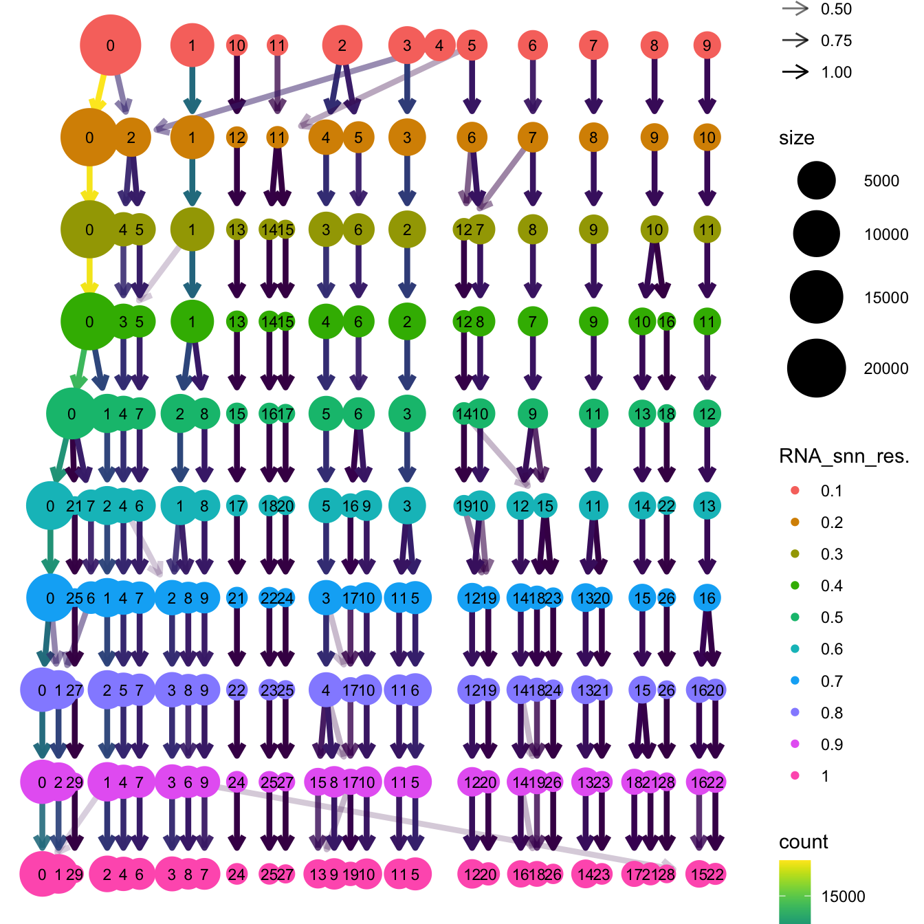
| Version | Author | Date |
|---|---|---|
| 6d2b67f | Gunjan Dixit | 2024-12-24 |
Based on the clustering tree, we chose an intermediate/optimum resolution where the clustering results are the most stable, with the least amount of shuffling cells.
opt_res <- "RNA_snn_res.0.5"
n <- nlevels(seu_obj$RNA_snn_res.0.5)
seu_obj$RNA_snn_res.0.5 <- factor(seu_obj$RNA_snn_res.0.5, levels = seq(0,n-1))
seu_obj$seurat_clusters <- NULL
seu_obj$cluster <- seu_obj$RNA_snn_res.0.5
Idents(seu_obj) <- seu_obj$cluster
UMAP after clustering
Defining colours for each cell-type to be consistent with other age-related/cell type composition plots.
my_colors <- c(
  "B cells" = "steelblue",
  "CD4 T cells" = "brown",
  "Double negative T cells" = "gold",
  "CD8 T cells" = "lightgreen",
  "Pre B/T cells" = "orchid",
  "Innate lymphoid cells" = "tan",
  "Natural Killer cells" = "blueviolet",
  "Macrophages" = "green4",
  "Cycling T cells" = "turquoise",
  "Dendritic cells" = "grey80",
  "Gamma delta T cells" = "mediumvioletred",
  "Epithelial lineage" = "darkorange",
  "Granulocytes" = "olivedrab",
  "Fibroblast lineage" = "lavender",
  "None" = "white",
  "Monocytes" = "peachpuff",
  "Endothelial lineage" = "cadetblue",
  "SMG duct" = "lightpink",
  "Neuroendocrine" = "skyblue",
  "Doublet query/Other" = "#d62728"
)
UMAP displaying clusters at opt_res resolution and Broad
cell Labels Level 3.
p1 <- DimPlot(seu_obj, reduction = "umap", raster = FALSE ,repel = TRUE, label = TRUE,label.size = 3.5, group.by = opt_res) +  NoLegend()

p2 <- DimPlot(seu_obj, reduction = "umap", raster = FALSE, repel = TRUE, label = TRUE, label.size = 3.5, group.by = "Broad_cell_label_3") + NoLegend() +
  scale_colour_manual(values = my_colors) +
  ggtitle(paste0(tissue, ": UMAP"))


p1 / p2 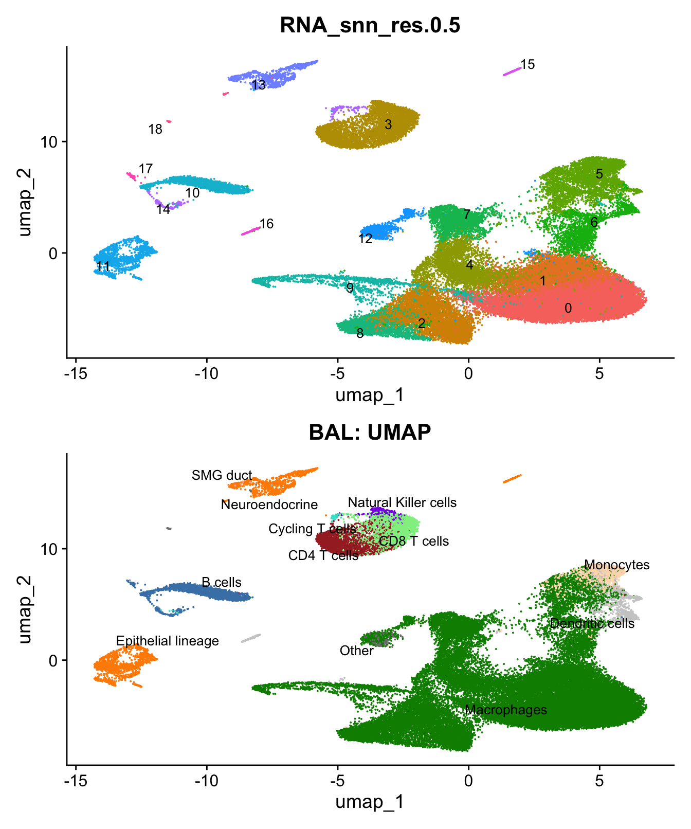
| Version | Author | Date |
|---|---|---|
| 6d2b67f | Gunjan Dixit | 2024-12-24 |
Save batch corrected Object
out1 <- here("output",
            "RDS", "AllBatches_Clustering_SEUs_v2",
             paste0("G000231_Neeland_",tissue,".Clusters.SEU.rds"))
#dir.create(out1)
if (!file.exists(out1)) {
  saveRDS(seu_obj, file = out1)
}
Marker Gene Analysis
The marker genes for this reclustering can be found here-
#seu_obj <- JoinLayers(seu_obj)
paed.markers <- FindAllMarkers(seu_obj, only.pos = TRUE, min.pct = 0.25, logfc.threshold = 0.25)
Extracting top 5 genes per cluster for visualization. The ‘top5’ contains the top 5 genes with the highest weighted average avg_log2FC within each cluster and the ‘best.wilcox.gene.per.cluster’ contains the single best gene with the highest weighted average avg_log2FC for each cluster.
paed.markers %>%
    group_by(cluster) %>% unique() %>%
    top_n(n = 5, wt = avg_log2FC) -> top5

paed.markers %>%
    group_by(cluster) %>%
    slice_head(n=1) %>%
    pull(gene) -> best.wilcox.gene.per.cluster

best.wilcox.gene.per.cluster
[1] "THBS1" "TMEM74B" "DEFB1" "IL32" "ABCA1" "SERPINB9"
[7] "VCAN" "CXCL2" "MT-ND5" "TK1" "CD79A" "CTXN1"
[13] "SLC11A1" "KRT7" "SEPTIN1" "KRT13" "GZMB" "MZB1"
[19] "KIT" Marker gene expression in clusters
This heatmap depicts the expression of top five genes in each cluster.
DoHeatmap(seu_obj, features = top5$gene) + NoLegend()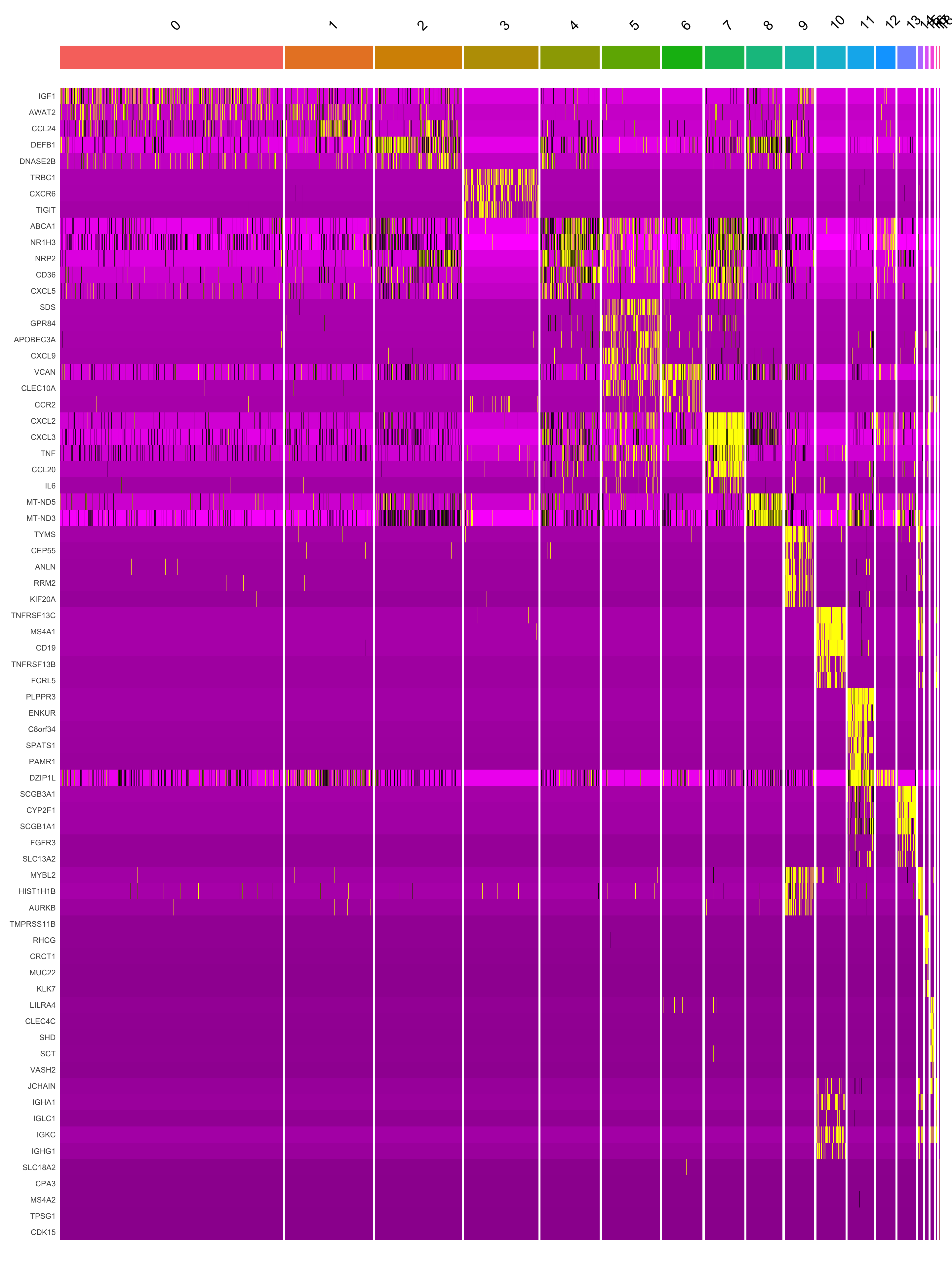
| Version | Author | Date |
|---|---|---|
| 6d2b67f | Gunjan Dixit | 2024-12-24 |
Violin plot shows the expression of top marker gene per cluster.
VlnPlot(seu_obj, features=best.wilcox.gene.per.cluster, ncol = 2, raster = FALSE, pt.size = FALSE)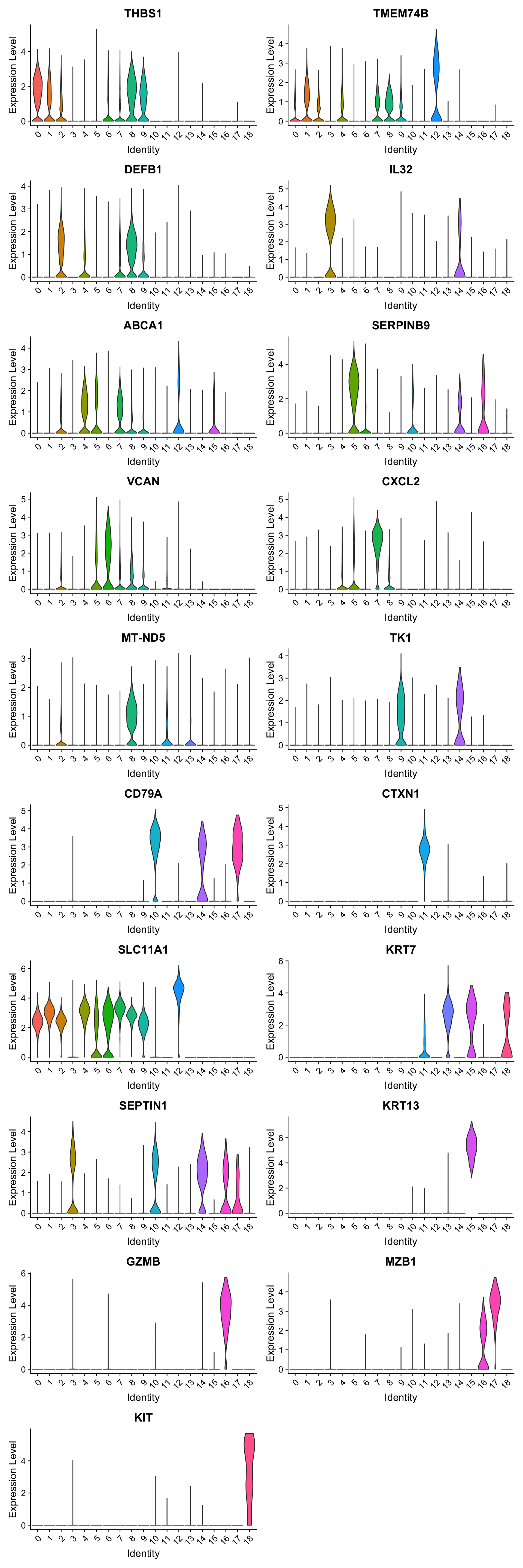
| Version | Author | Date |
|---|---|---|
| 6d2b67f | Gunjan Dixit | 2024-12-24 |
Feature plot shows the expression of top marker genes per cluster.
FeaturePlot(seu_obj,features=best.wilcox.gene.per.cluster, reduction = 'umap', raster = FALSE, ncol = 2)
| Version | Author | Date |
|---|---|---|
| 6d2b67f | Gunjan Dixit | 2024-12-24 |
Extract markers for each cluster
This section extracts marker genes for each cluster and save them as a CSV file.
out_markers <- here("output",
            "CSV_v2", tissue,
            paste(tissue,"_Marker_gene_clusters.",opt_res, sep = ""))

dir.create(out_markers, recursive = TRUE, showWarnings = FALSE)

for (cl in unique(paed.markers$cluster)) {
  cluster_data <- paed.markers %>% dplyr::filter(cluster == cl)
  file_name <- here(out_markers, paste0("G000231_Neeland_",tissue, "_cluster_", cl, ".csv"))
  write.csv(cluster_data, file = file_name)
}
Using old labels to annotate cell types
out1 <- here("output",
"RDS", "AllBatches_Clustering_SEUs",
paste0("G000231_Neeland_",tissue,".Clusters.SEU.rds"))
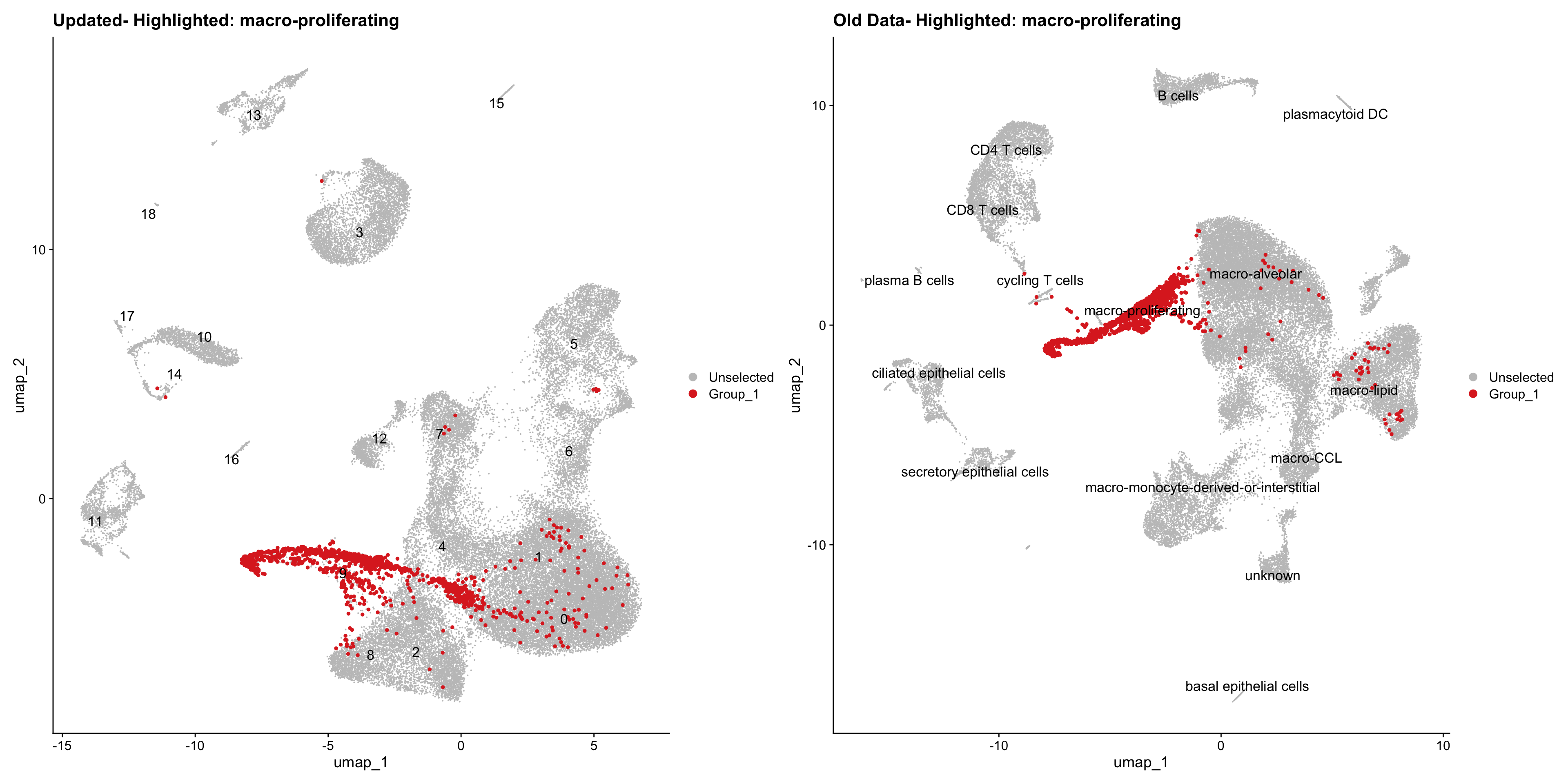
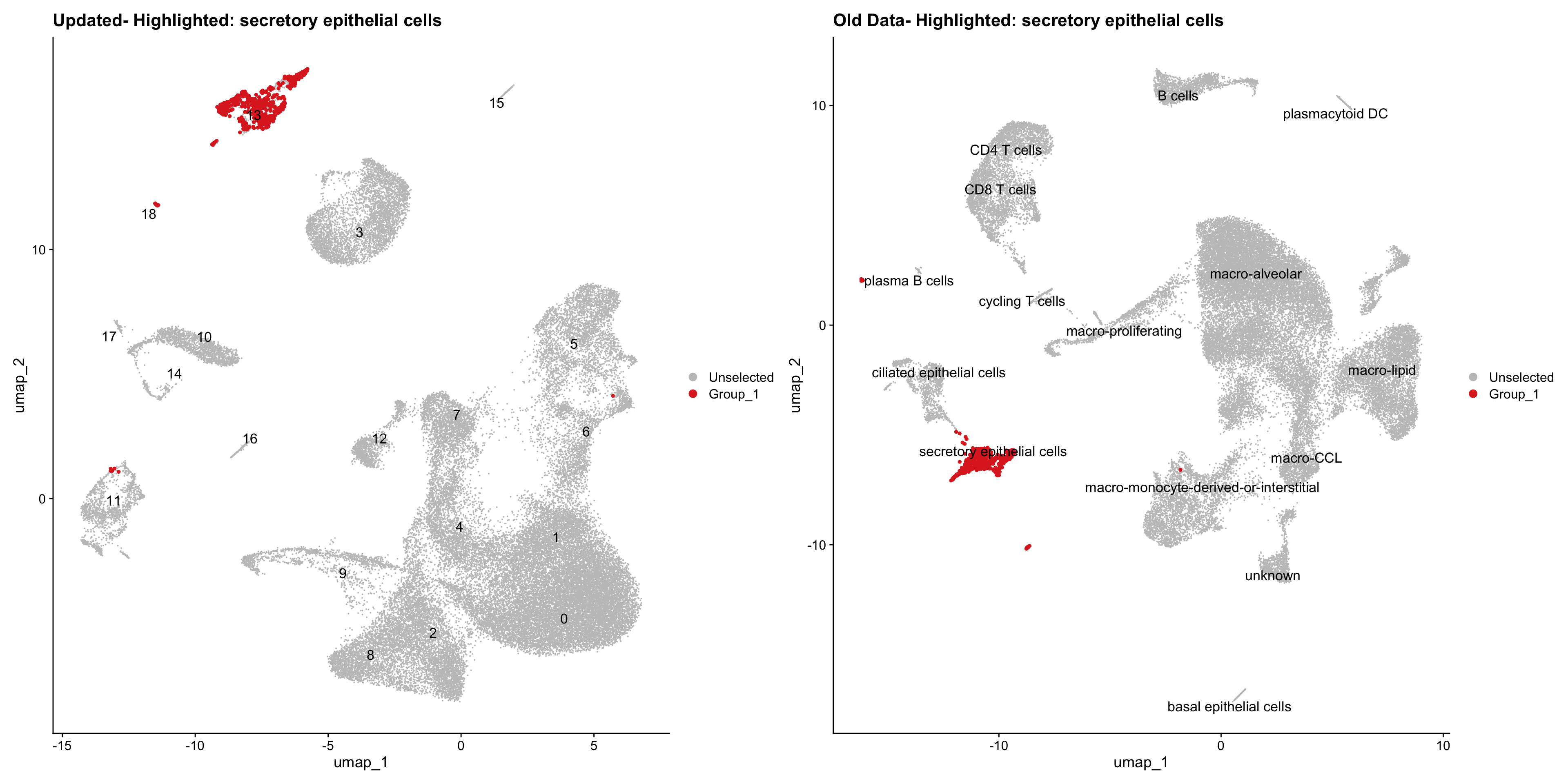
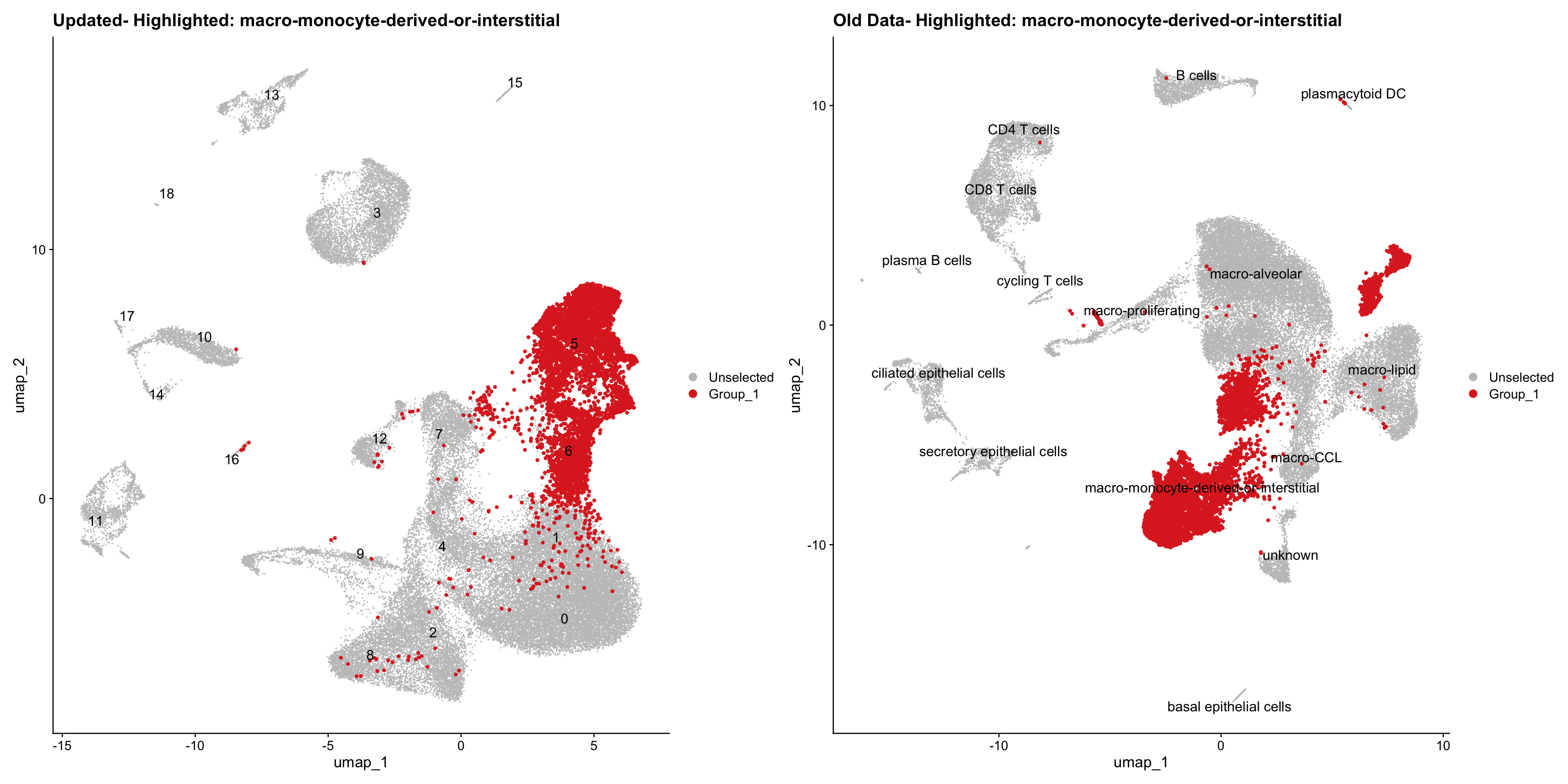
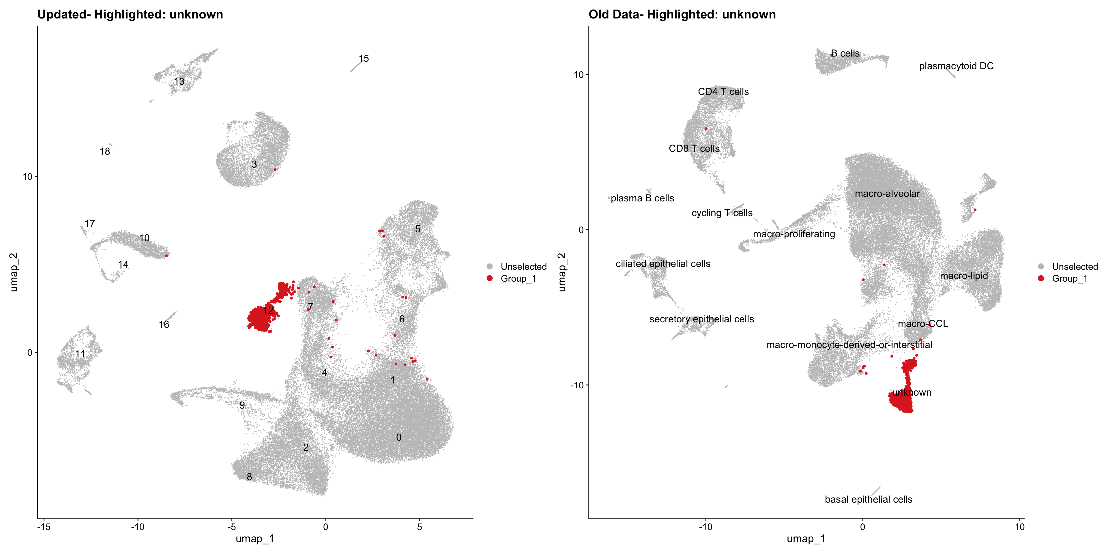
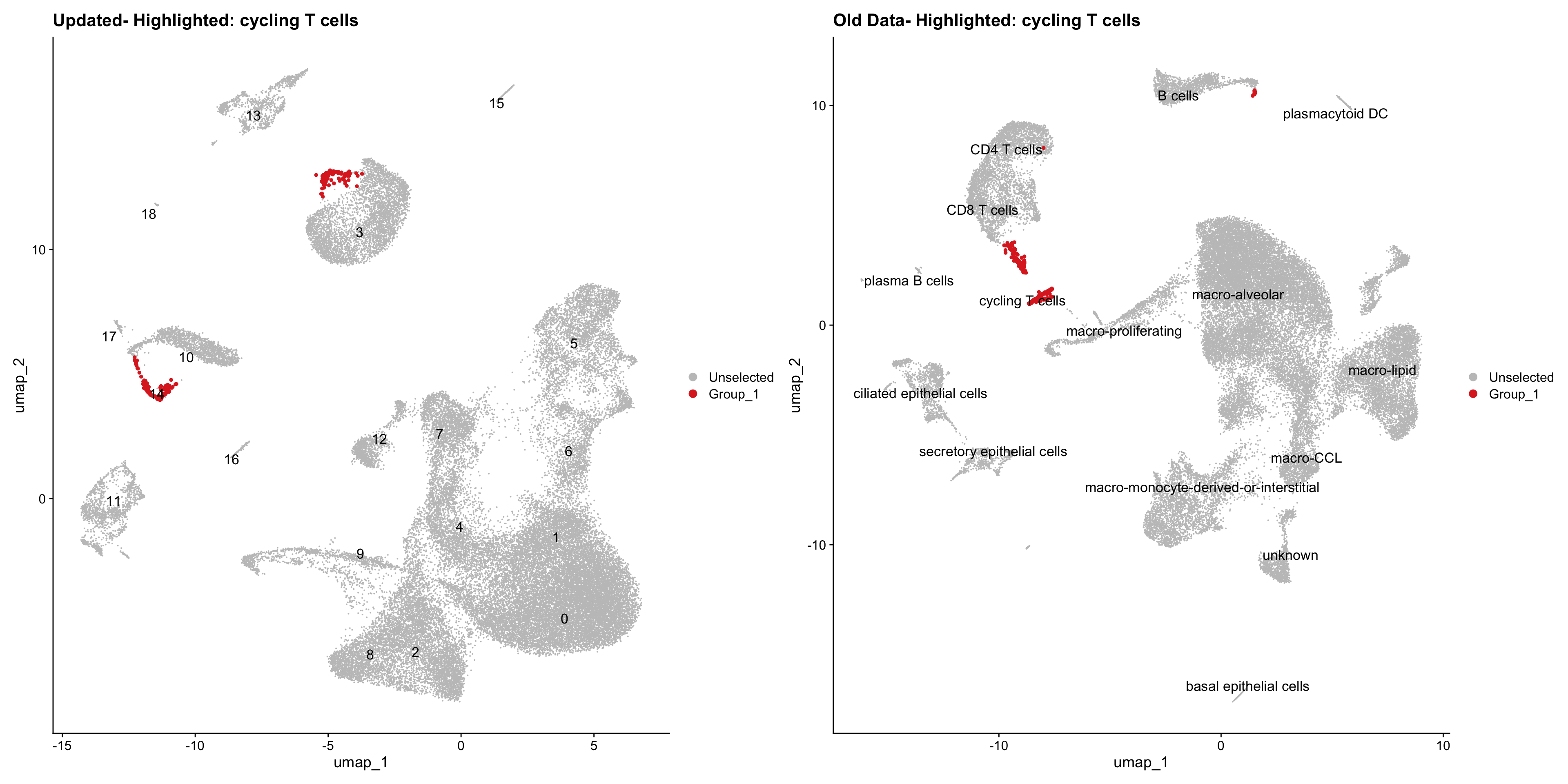
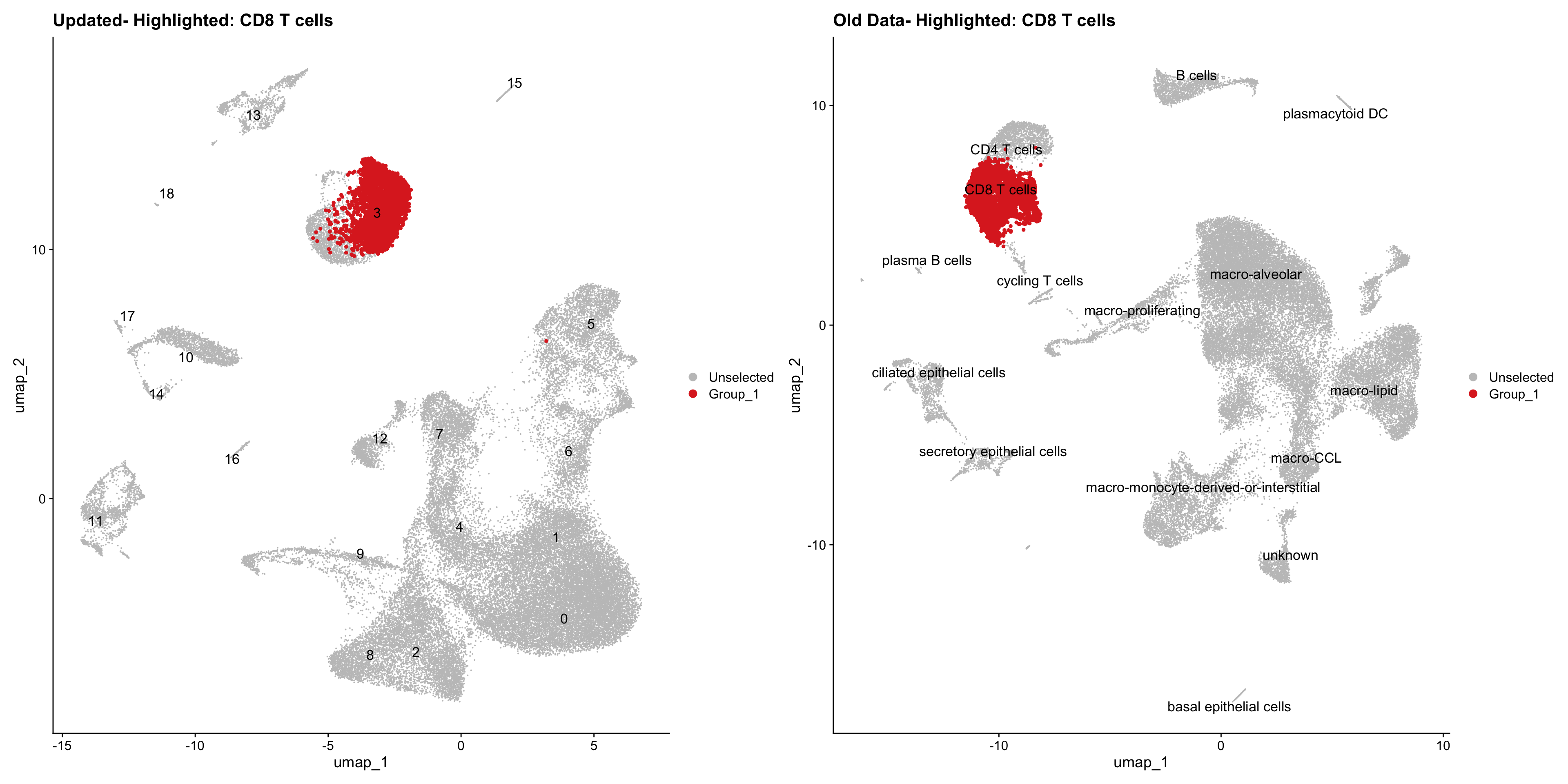
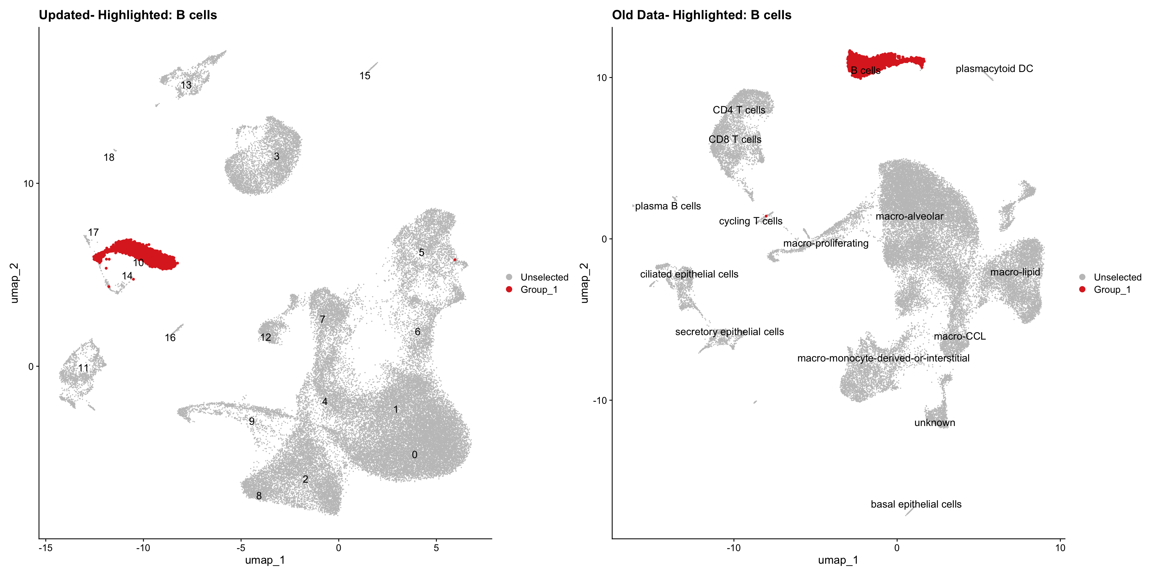
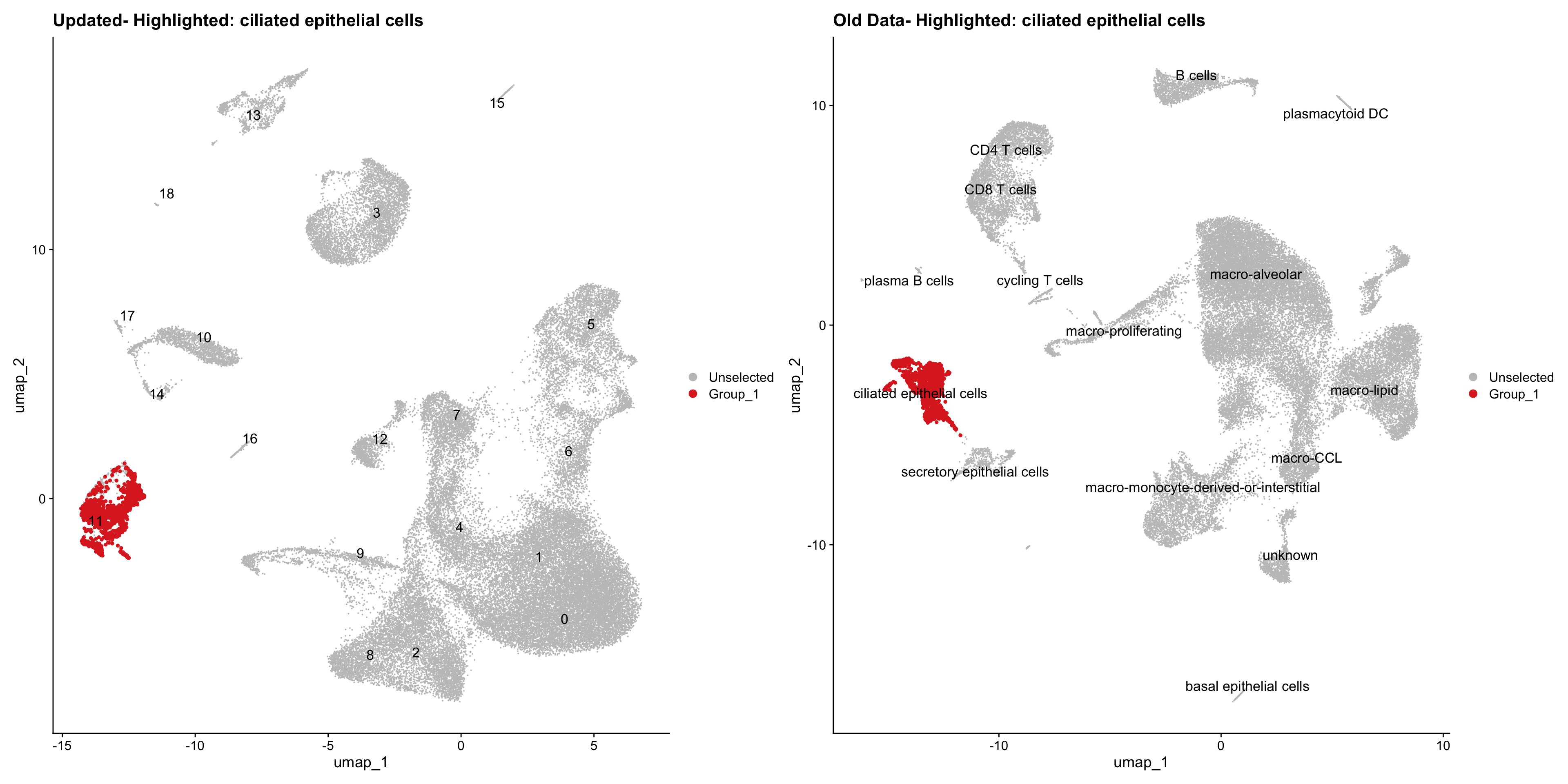
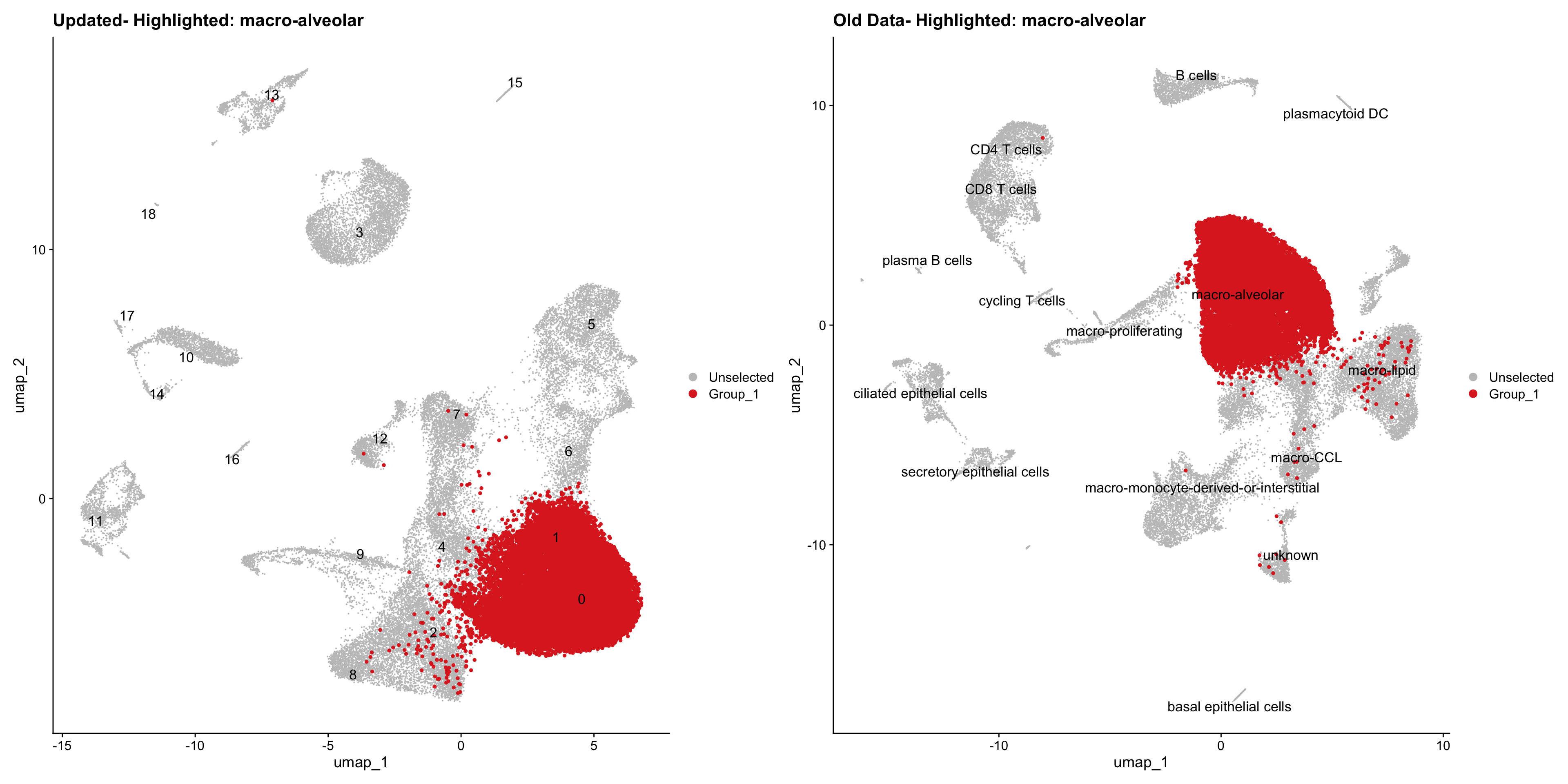
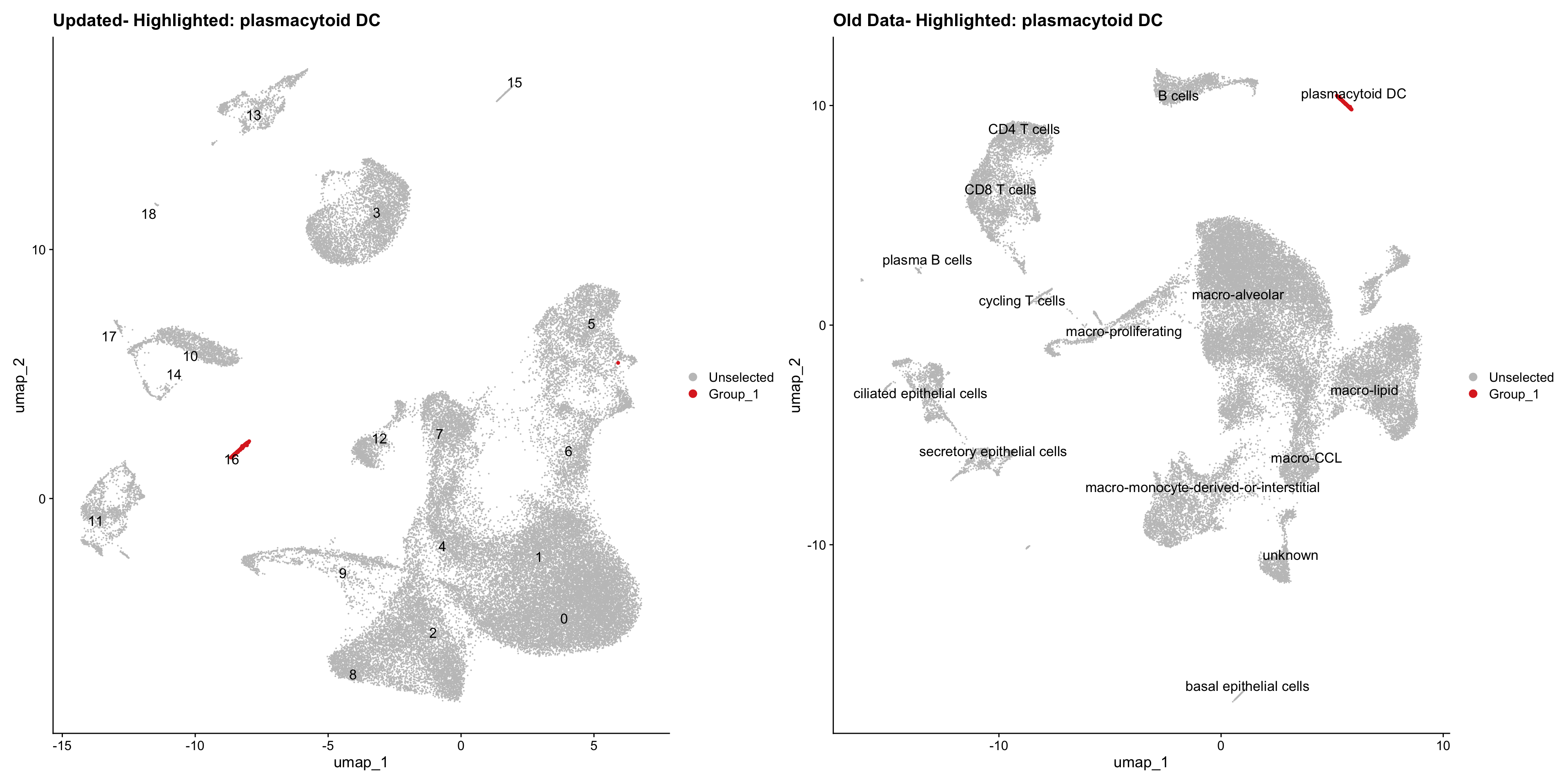
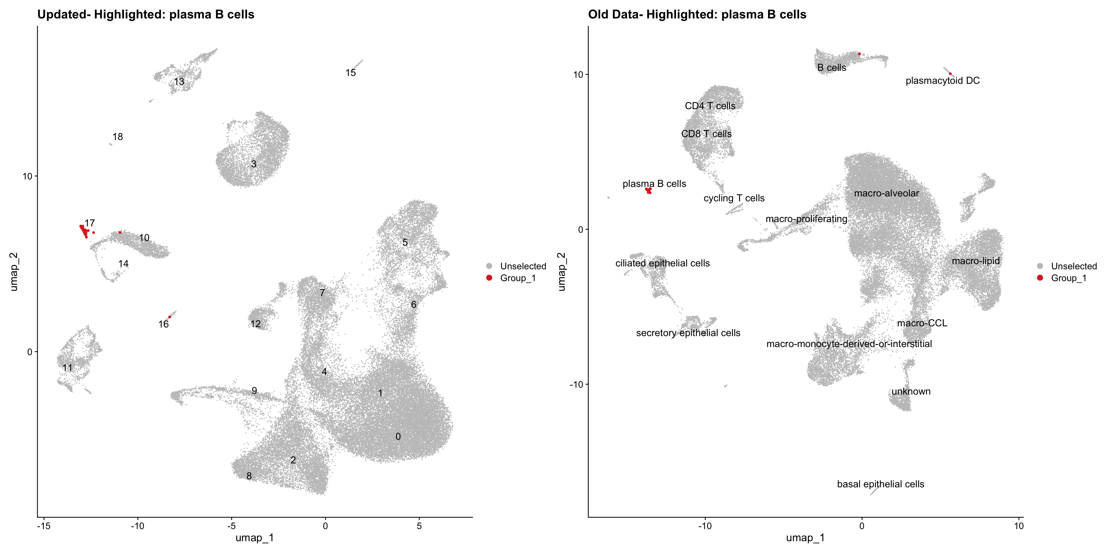
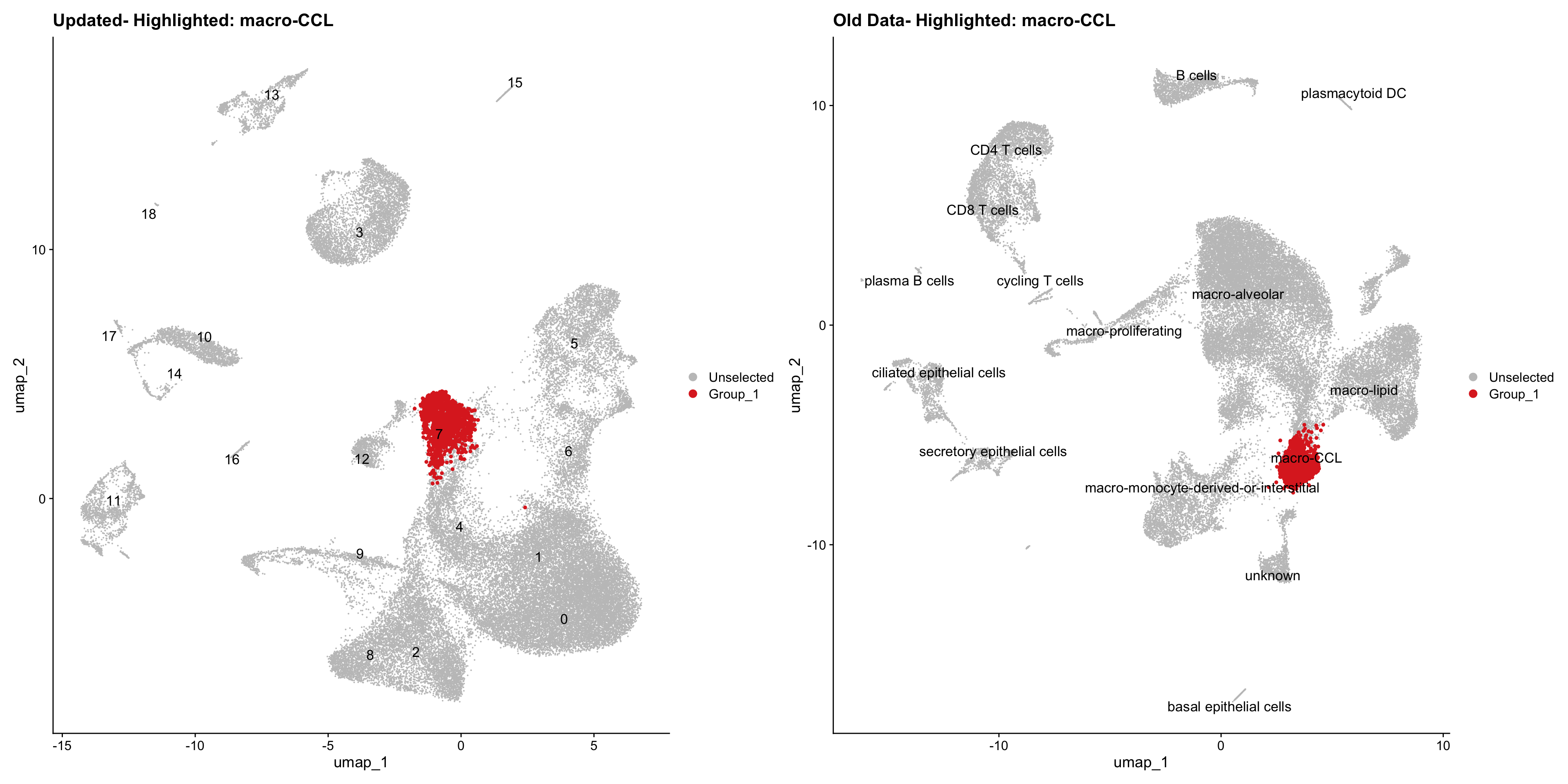
old_obj <- readRDS(out1)cell_types <- unique(old_obj$cell_labels)
for (cell_type in cell_types) {
cl_cells <- WhichCells(old_obj, idents = cell_type)
p <- DimPlot(
seu_obj,
reduction = "umap",
label = TRUE,
label.size = 4.5,
repel = TRUE,
raster = FALSE,
cells.highlight = cl_cells
) +
ggtitle(paste("Updated- Highlighted:", cell_type))
p1 <- DimPlot(
old_obj,
reduction = "umap",
label = T,
label.size = 4.5,
repel = TRUE,
raster = FALSE,
cells.highlight = cl_cells
) +
ggtitle(paste("Old Data- Highlighted:", cell_type))
print(p | p1)
}
| Version | Author | Date |
|---|---|---|
| 6d2b67f | Gunjan Dixit | 2024-12-24 |
| Version | Author | Date |
|---|---|---|
| 6d2b67f | Gunjan Dixit | 2024-12-24 |
| Version | Author | Date |
|---|---|---|
| 6d2b67f | Gunjan Dixit | 2024-12-24 |
| Version | Author | Date |
|---|---|---|
| 6d2b67f | Gunjan Dixit | 2024-12-24 |
| Version | Author | Date |
|---|---|---|
| 6d2b67f | Gunjan Dixit | 2024-12-24 |
| Version | Author | Date |
|---|---|---|
| 6d2b67f | Gunjan Dixit | 2024-12-24 |
| Version | Author | Date |
|---|---|---|
| 6d2b67f | Gunjan Dixit | 2024-12-24 |
| Version | Author | Date |
|---|---|---|
| 6d2b67f | Gunjan Dixit | 2024-12-24 |
| Version | Author | Date |
|---|---|---|
| 6d2b67f | Gunjan Dixit | 2024-12-24 |
| Version | Author | Date |
|---|---|---|
| 6d2b67f | Gunjan Dixit | 2024-12-24 |
| Version | Author | Date |
|---|---|---|
| 6d2b67f | Gunjan Dixit | 2024-12-24 |
| Version | Author | Date |
|---|---|---|
| 6d2b67f | Gunjan Dixit | 2024-12-24 |
| Version | Author | Date |
|---|---|---|
| 6d2b67f | Gunjan Dixit | 2024-12-24 |
| Version | Author | Date |
|---|---|---|
| 6d2b67f | Gunjan Dixit | 2024-12-24 |
| Version | Author | Date |
|---|---|---|
| 6d2b67f | Gunjan Dixit | 2024-12-24 |
Updated cell-type labels (all clusters)
cell_labels <- readxl::read_excel(here("data/cell_labels_Mel_v4_Dec2024/earlyAIR_BAL_all.xlsx"), sheet = "all_clusters")

new_cluster_names <- cell_labels %>%
  dplyr::select(cluster, annotation) %>%
  deframe()

seu_obj <- RenameIdents(seu_obj, new_cluster_names)
seu_obj@meta.data$cell_labels <- Idents(seu_obj)

p3 <- DimPlot(seu_obj, reduction = "umap", raster = FALSE, repel = TRUE, label = TRUE, label.size = 3.5) + ggtitle(paste0(tissue, ": UMAP with Updated cell types"))

p3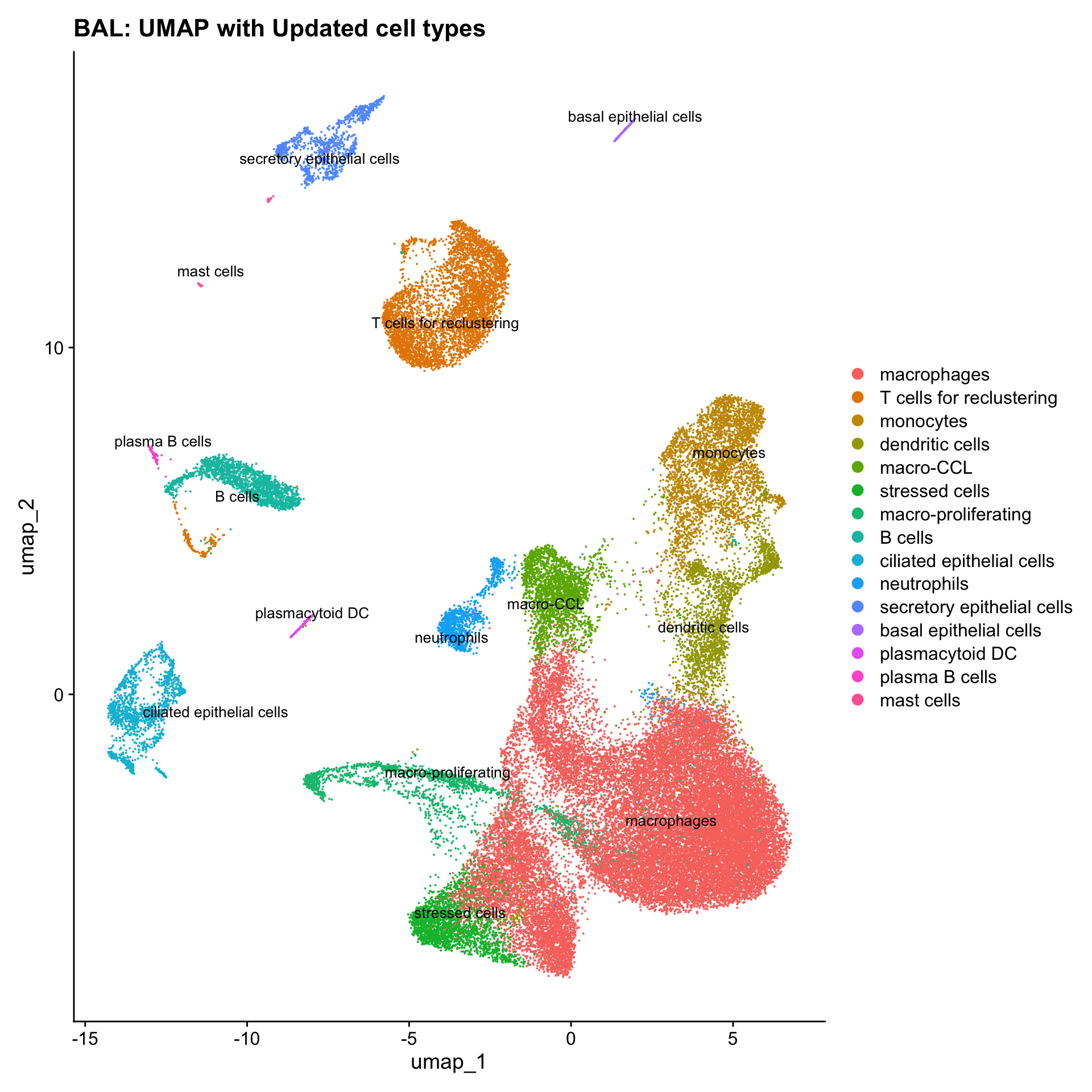
| Version | Author | Date |
|---|---|---|
| 3595ad0 | Gunjan Dixit | 2025-01-07 |
Summary Plots
seu_obj@meta.data$donor <- sub("_\\d+$", "", seu_obj@meta.data$donor_id)
palette1 <- paletteer::paletteer_d("ggthemes::Classic_20")
palette2 <- paletteer::paletteer_d("Polychrome::light")
combined_palette <- unique(c(palette1, palette2))

p1 <- seu_obj@meta.data %>%
  dplyr::select(!!sym(opt_res), donor) %>%
  group_by(!!sym(opt_res), donor) %>%
  summarise(num = n()) %>%
  mutate(prop = num / sum(num)) %>%
  ggplot(aes(x = !!sym(opt_res), y = prop * 100,
             fill = donor)) +
  geom_bar(stat = "identity") +
  theme(axis.text.x = element_text(angle = 90,
                                   vjust = 0.5,
                                   hjust = 1,
                                   size = 8)) +
  labs(y = "% Cells", fill = "donor") +
  scale_fill_manual(values = combined_palette)
`summarise()` has grouped output by 'RNA_snn_res.0.5'. You can override using
the `.groups` argument.p2 <- seu_obj@meta.data %>%
dplyr::select(!!sym(opt_res), sample_id) %>%
group_by(!!sym(opt_res), sample_id) %>%
summarise(num = n()) %>%
mutate(prop = num / sum(num)) %>%
ggplot(aes(x = !!sym(opt_res), y = prop * 100,
fill = sample_id)) +
geom_bar(stat = "identity") +
theme(axis.text.x = element_text(angle = 90,
vjust = 0.5,
hjust = 1,
size = 8)) +
labs(y = "% Cells", fill = "sample_id") +
scale_fill_manual(values = combined_palette)`summarise()` has grouped output by 'RNA_snn_res.0.5'. You can override using
the `.groups` argument.# Combine the plots
p <- (p1 / p2) & theme( legend.text = element_text(size = 8),
legend.key.size = unit(3, "mm"))
p + plot_annotation(title = paste0(tissue, ": Tcell subclusters"))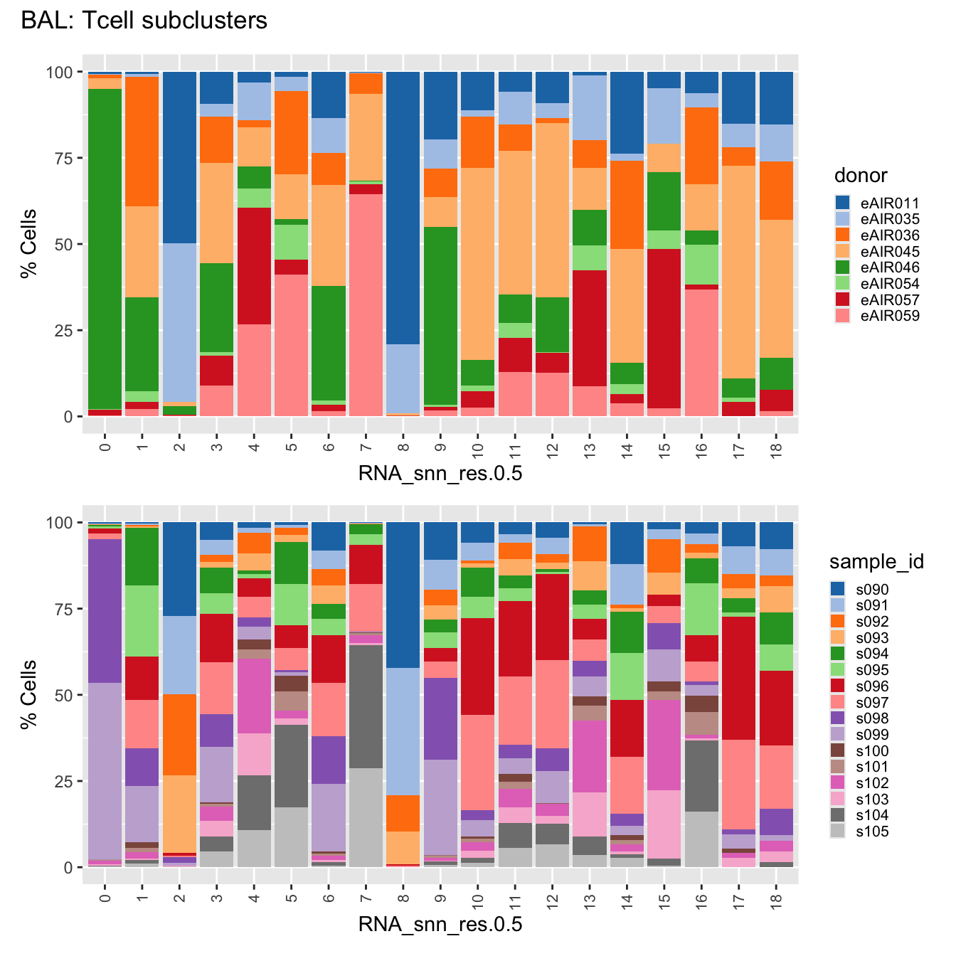
labels <- c( "predicted.ann_level_1","predicted.ann_level_2", "predicted.ann_level_3", "predicted.ann_level_4", "predicted.ann_level_5","predicted.ann_finest_level", "cell_labels")

p <- vector("list",length(labels))
for(label in labels){
  seu_obj@meta.data %>%
    ggplot(aes(x = !!sym(label),
               fill = !!sym(label))) +
    geom_bar() +
    geom_text(aes(label = ..count..), stat = "count",
              vjust = -0.5, colour = "black", size = 2) +
    scale_y_log10() +
    theme(axis.text.x = element_blank(),
          axis.title.x = element_blank(),
          axis.ticks.x = element_blank()) +
    NoLegend() +
    labs(y = "No. Cells (log scale)") -> p1

  seu_obj@meta.data %>%
    dplyr::select(!!sym(label), donor) %>%
    group_by(!!sym(label), donor) %>%
    summarise(num = n()) %>%
    mutate(prop = num / sum(num)) %>%
  ggplot(aes(x = !!sym(label), y = prop * 100,
             fill = donor)) +
    geom_bar(stat = "identity") +
    theme(axis.text.x = element_text(angle = 90,
                                     vjust = 0.5,
                                     hjust = 1,
                                     size = 8)) +
    labs(y = "% Cells", fill = "Donor") +
  scale_fill_manual(values = combined_palette) -> p2

  (p1 / p2) & theme(legend.text = element_text(size = 8),
                  legend.key.size = unit(3, "mm")) -> p[[label]]
}
`summarise()` has grouped output by 'predicted.ann_level_1'. You can override
using the `.groups` argument.
`summarise()` has grouped output by 'predicted.ann_level_2'. You can override
using the `.groups` argument.
`summarise()` has grouped output by 'predicted.ann_level_3'. You can override
using the `.groups` argument.
`summarise()` has grouped output by 'predicted.ann_level_4'. You can override
using the `.groups` argument.
`summarise()` has grouped output by 'predicted.ann_level_5'. You can override
using the `.groups` argument.
`summarise()` has grouped output by 'predicted.ann_finest_level'. You can
override using the `.groups` argument.
`summarise()` has grouped output by 'cell_labels'. You can override using the
`.groups` argument.p[[1]]
NULL
[[2]]
NULL
[[3]]
NULL
[[4]]
NULL
[[5]]
NULL
[[6]]
NULL
[[7]]
NULL
$predicted.ann_level_1Warning: The dot-dot notation (`..count..`) was deprecated in ggplot2 3.4.0.
ℹ Please use `after_stat(count)` instead.
This warning is displayed once every 8 hours.
Call `lifecycle::last_lifecycle_warnings()` to see where this warning was
generated.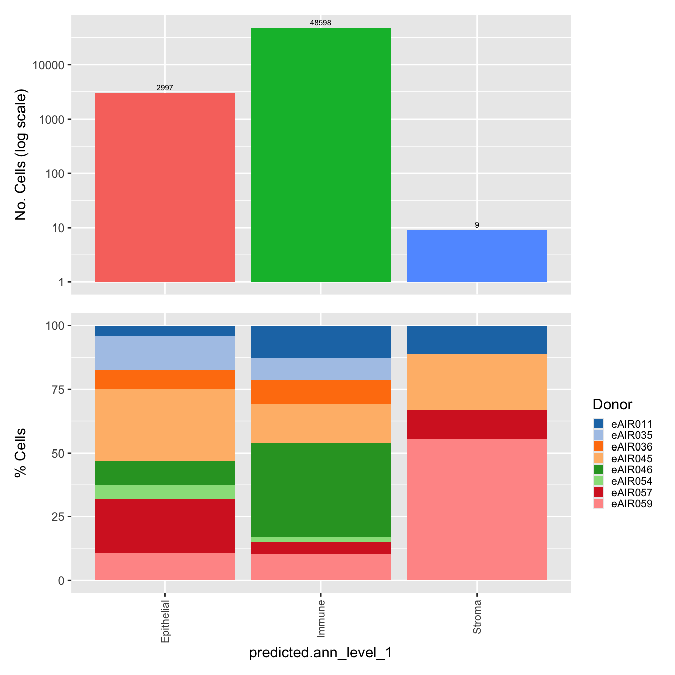
| Version | Author | Date |
|---|---|---|
| 3595ad0 | Gunjan Dixit | 2025-01-07 |
$predicted.ann_level_2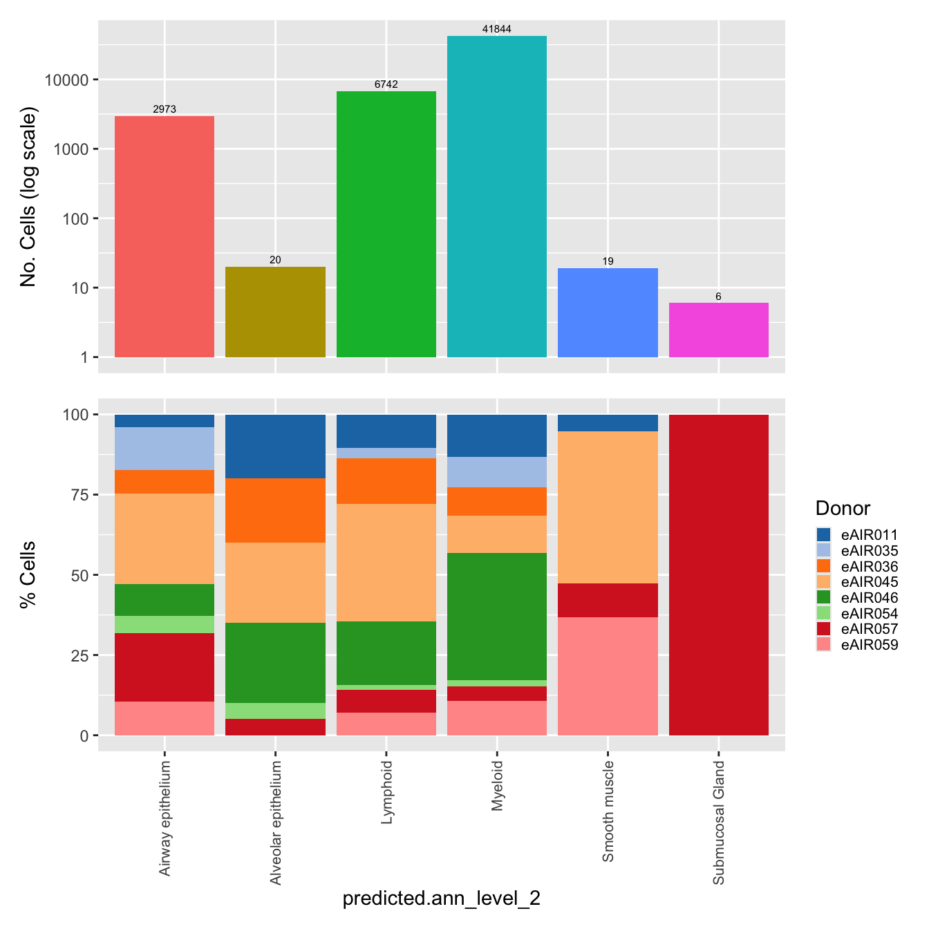
| Version | Author | Date |
|---|---|---|
| 3595ad0 | Gunjan Dixit | 2025-01-07 |
$predicted.ann_level_3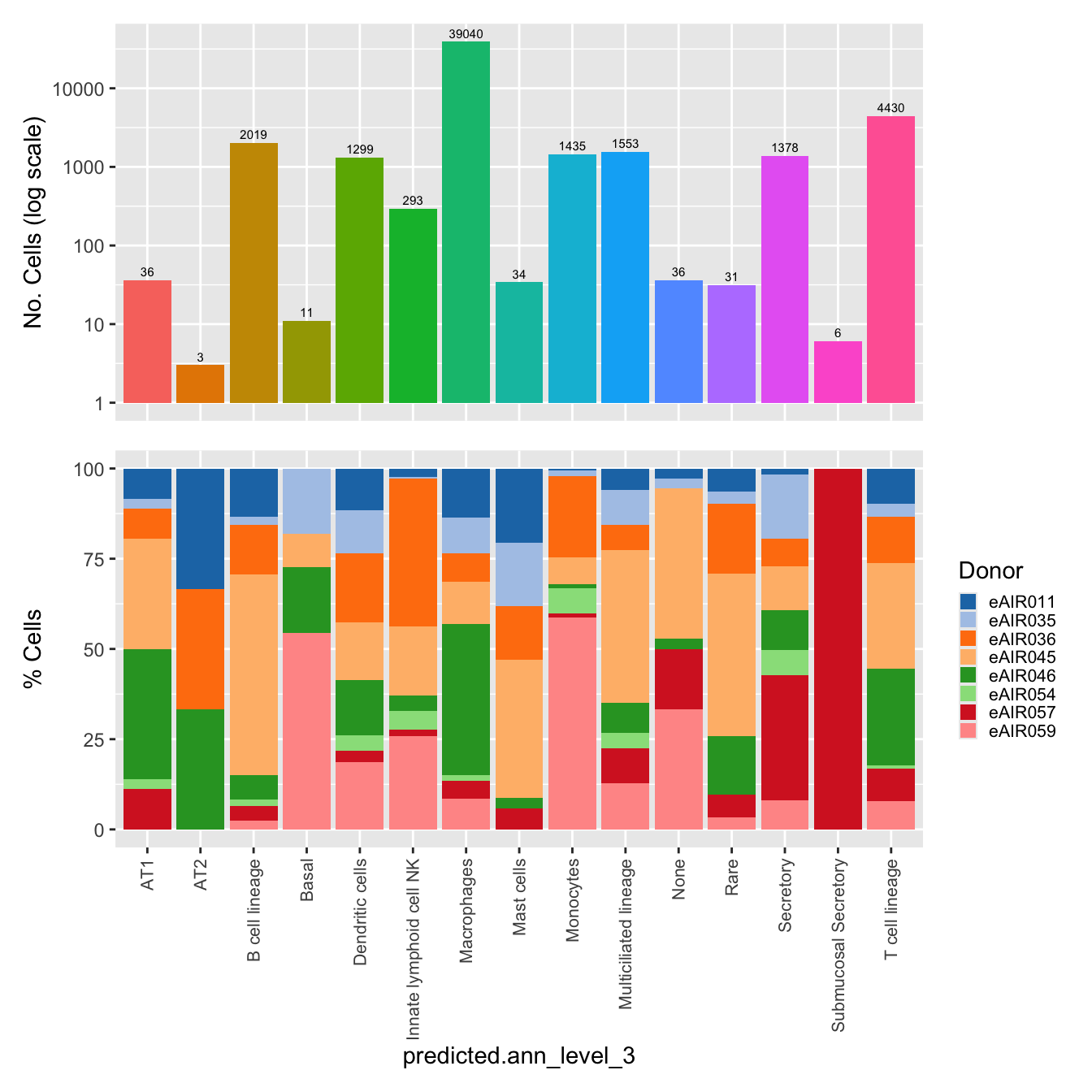
| Version | Author | Date |
|---|---|---|
| 3595ad0 | Gunjan Dixit | 2025-01-07 |
$predicted.ann_level_4
| Version | Author | Date |
|---|---|---|
| 3595ad0 | Gunjan Dixit | 2025-01-07 |
$predicted.ann_level_5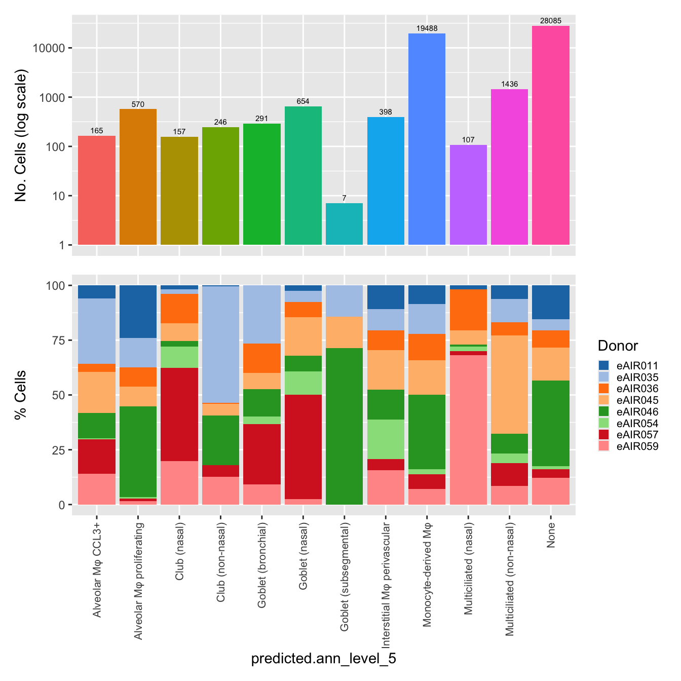
| Version | Author | Date |
|---|---|---|
| 3595ad0 | Gunjan Dixit | 2025-01-07 |
$predicted.ann_finest_level
| Version | Author | Date |
|---|---|---|
| 3595ad0 | Gunjan Dixit | 2025-01-07 |
$cell_labels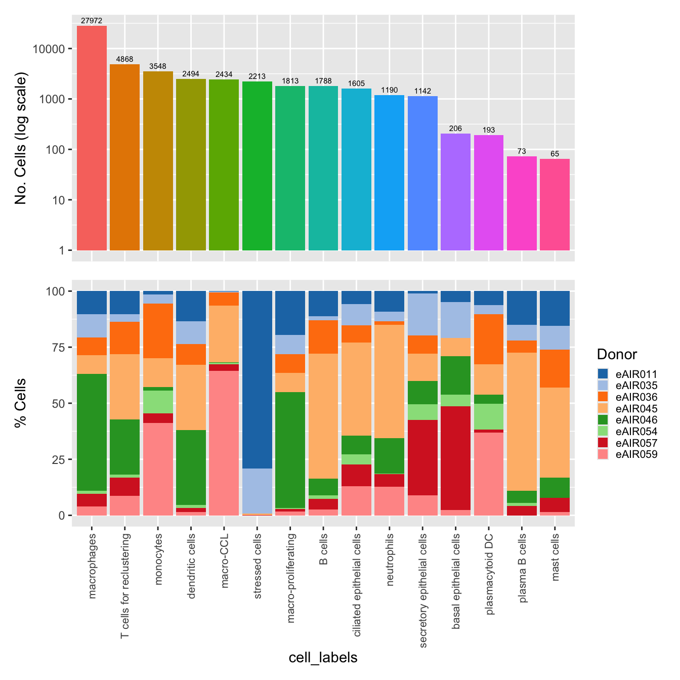
| Version | Author | Date |
|---|---|---|
| 3595ad0 | Gunjan Dixit | 2025-01-07 |
Reclustering Tcell polulation
This includes CD4 T cell, CD8 T cell, NK cell, NK-T cell, proliferating or cycling T/NK cell.
The marker genes for this reclustering can be found here-
#sub_clusters <- c(3,14)
#idx <- which(seu_obj$cluster %in% sub_clusters)
idx <- which(Idents(seu_obj) %in% "T cells for reclustering")
paed_sub <- seu_obj[,idx]
mito_genes <- grep("^MT-", rownames(paed_sub), value = TRUE)
paed_sub <- subset(paed_sub, features = setdiff(rownames(paed_sub), mito_genes))
paed_sub
An object of class Seurat
17518 features across 4868 samples within 1 assay
Active assay: RNA (17518 features, 1991 variable features)
3 layers present: counts, data, scale.data
2 dimensional reductions calculated: pca, umappaed_sub <- paed_sub %>%
NormalizeData() %>%
FindVariableFeatures() %>%
ScaleData() %>%
RunPCA()
paed_sub <- RunUMAP(paed_sub, dims = 1:30, reduction = "pca", reduction.name = "umap.tcell")
meta_data_columns <- colnames(paed_sub@meta.data)
columns_to_remove <- grep("^RNA_snn_res", meta_data_columns, value = TRUE)
paed_sub@meta.data <- paed_sub@meta.data[, !(colnames(paed_sub@meta.data) %in% columns_to_remove)]
resolutions <- seq(0.1, 1, by = 0.1)
paed_sub <- FindNeighbors(paed_sub, reduction = "pca", dims = 1:30)
paed_sub <- FindClusters(paed_sub, resolution = resolutions, algorithm = 3)Modularity Optimizer version 1.3.0 by Ludo Waltman and Nees Jan van Eck
Number of nodes: 4868
Number of edges: 185935
Running smart local moving algorithm...
Maximum modularity in 10 random starts: 0.9356
Number of communities: 5
Elapsed time: 2 seconds
Modularity Optimizer version 1.3.0 by Ludo Waltman and Nees Jan van Eck
Number of nodes: 4868
Number of edges: 185935
Running smart local moving algorithm...
Maximum modularity in 10 random starts: 0.9100
Number of communities: 9
Elapsed time: 2 seconds
Modularity Optimizer version 1.3.0 by Ludo Waltman and Nees Jan van Eck
Number of nodes: 4868
Number of edges: 185935
Running smart local moving algorithm...
Maximum modularity in 10 random starts: 0.8907
Number of communities: 12
Elapsed time: 2 seconds
Modularity Optimizer version 1.3.0 by Ludo Waltman and Nees Jan van Eck
Number of nodes: 4868
Number of edges: 185935
Running smart local moving algorithm...
Maximum modularity in 10 random starts: 0.8740
Number of communities: 11
Elapsed time: 2 seconds
Modularity Optimizer version 1.3.0 by Ludo Waltman and Nees Jan van Eck
Number of nodes: 4868
Number of edges: 185935
Running smart local moving algorithm...
Maximum modularity in 10 random starts: 0.8576
Number of communities: 11
Elapsed time: 2 seconds
Modularity Optimizer version 1.3.0 by Ludo Waltman and Nees Jan van Eck
Number of nodes: 4868
Number of edges: 185935
Running smart local moving algorithm...
Maximum modularity in 10 random starts: 0.8422
Number of communities: 13
Elapsed time: 1 seconds
Modularity Optimizer version 1.3.0 by Ludo Waltman and Nees Jan van Eck
Number of nodes: 4868
Number of edges: 185935
Running smart local moving algorithm...
Maximum modularity in 10 random starts: 0.8295
Number of communities: 14
Elapsed time: 1 seconds
Modularity Optimizer version 1.3.0 by Ludo Waltman and Nees Jan van Eck
Number of nodes: 4868
Number of edges: 185935
Running smart local moving algorithm...
Maximum modularity in 10 random starts: 0.8194
Number of communities: 15
Elapsed time: 1 seconds
Modularity Optimizer version 1.3.0 by Ludo Waltman and Nees Jan van Eck
Number of nodes: 4868
Number of edges: 185935
Running smart local moving algorithm...
Maximum modularity in 10 random starts: 0.8093
Number of communities: 16
Elapsed time: 1 seconds
Modularity Optimizer version 1.3.0 by Ludo Waltman and Nees Jan van Eck
Number of nodes: 4868
Number of edges: 185935
Running smart local moving algorithm...
Maximum modularity in 10 random starts: 0.7997
Number of communities: 17
Elapsed time: 1 secondsDimHeatmap(paed_sub, dims = 1:10, cells = 500, balanced = TRUE)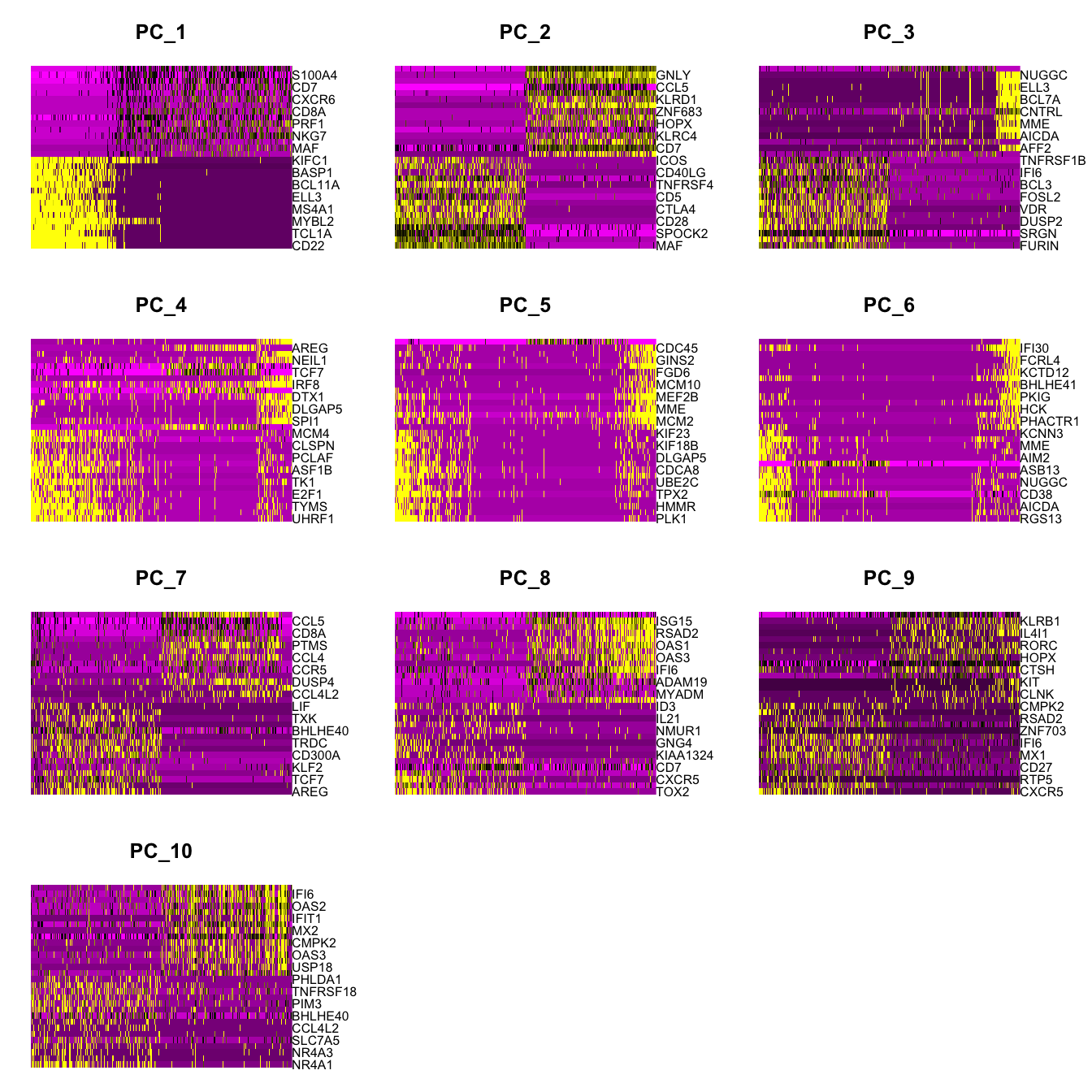
clustree(paed_sub, prefix = "RNA_snn_res.")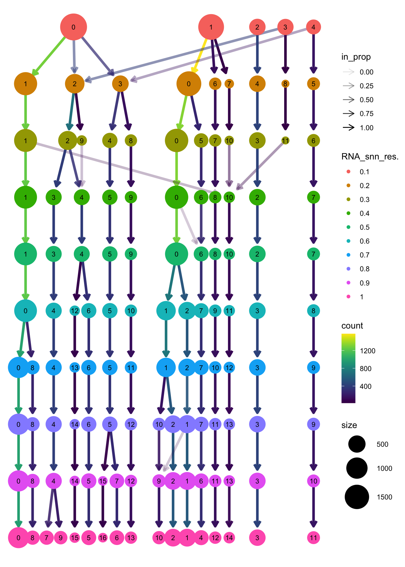
| Version | Author | Date |
|---|---|---|
| 6d2b67f | Gunjan Dixit | 2024-12-24 |
opt_res <- "RNA_snn_res.0.4"
n <- nlevels(paed_sub$RNA_snn_res.0.4)
paed_sub$RNA_snn_res.0.4 <- factor(paed_sub$RNA_snn_res.0.4, levels = seq(0,n-1))
paed_sub$seurat_clusters <- NULL
paed_sub$cluster <- paed_sub$RNA_snn_res.0.4
Idents(paed_sub) <- paed_sub$cluster
paed_sub.markers <- FindAllMarkers(paed_sub, only.pos = TRUE, min.pct = 0.25, logfc.threshold = 0.25)Calculating cluster 0Calculating cluster 1Calculating cluster 2Calculating cluster 3Calculating cluster 4Calculating cluster 5Calculating cluster 6Calculating cluster 7Calculating cluster 8Calculating cluster 9Calculating cluster 10paed_sub.markers %>%
group_by(cluster) %>% unique() %>%
top_n(n = 5, wt = avg_log2FC) -> top5
paed_sub.markers %>%
group_by(cluster) %>%
slice_head(n=1) %>%
pull(gene) -> best.wilcox.gene.per.cluster
best.wilcox.gene.per.cluster [1] "CD4" "CCL5" "NMUR1" "TCF7" "AREG" "GZMB" "MAF" "CD79A"
[9] "CXCR5" "TYMS" "CX3CR1"Feature plot shows the expression of top marker genes per cluster.
FeaturePlot(paed_sub,features=best.wilcox.gene.per.cluster, reduction = 'umap.tcell', raster = FALSE, ncol = 2, label = TRUE)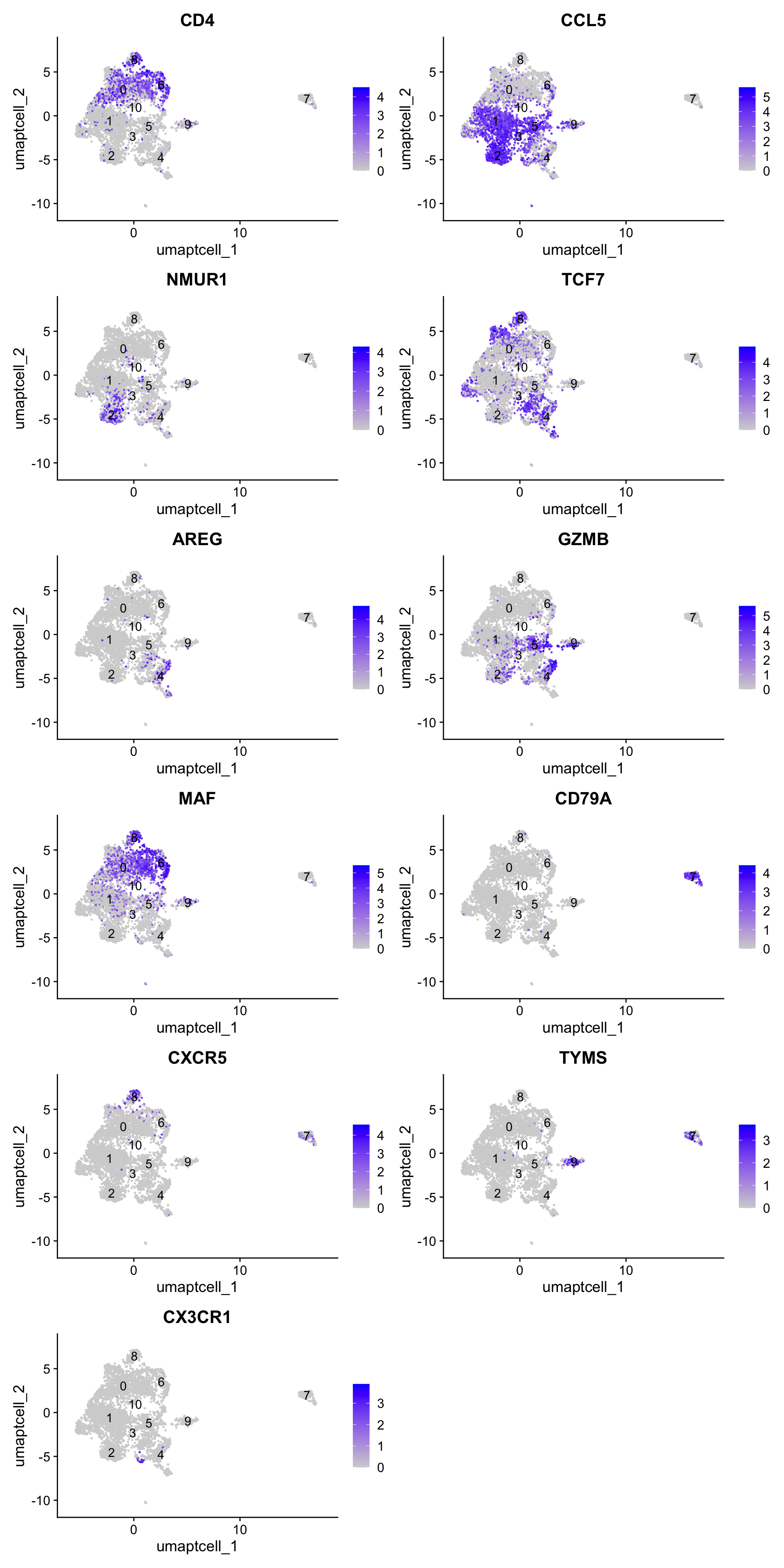
Top 10 marker genes from Seurat
## Seurat top markers
top10 <- paed_sub.markers %>%
    group_by(cluster) %>%
    top_n(n = 10, wt = avg_log2FC) %>%
    ungroup() %>%
    distinct(gene, .keep_all = TRUE) %>%
    arrange(cluster, desc(avg_log2FC))

cluster_colors <- paletteer::paletteer_d("pals::glasbey")[factor(top10$cluster)]

DotPlot(paed_sub,
        features = unique(top10$gene),
        group.by = opt_res,
        cols = c("azure1", "blueviolet"),
        dot.scale = 3, assay = "RNA") +
    RotatedAxis() +
    FontSize(y.text = 8, x.text = 12) +
    labs(y = element_blank(), x = element_blank()) +
    coord_flip() +
    theme(axis.text.y = element_text(color = cluster_colors)) +
    ggtitle("Top 10 marker genes per cluster (Seurat)")
Warning: Vectorized input to `element_text()` is not officially supported.
ℹ Results may be unexpected or may change in future versions of ggplot2.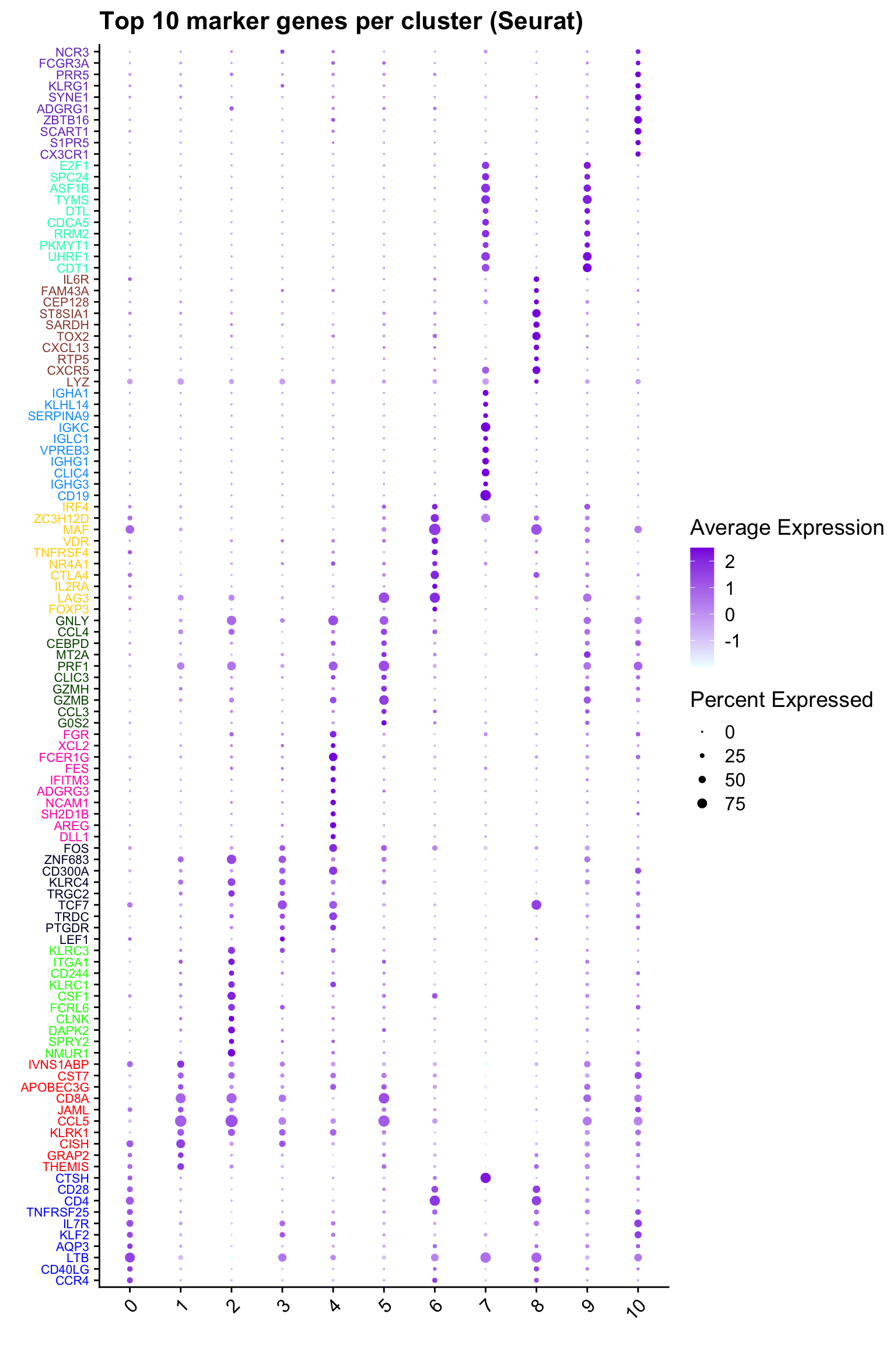
out_markers <- here("output",
            "CSV_v2", tissue,
            paste(tissue,"_Marker_genes_Reclustered_Tcell_population.",opt_res, sep = ""))

dir.create(out_markers, recursive = TRUE, showWarnings = FALSE)

for (cl in unique(paed_sub.markers$cluster)) {
  cluster_data <- paed_sub.markers %>% dplyr::filter(cluster == cl)
  file_name <- here(out_markers, paste0("G000231_Neeland_",tissue, "_cluster_", cl, ".csv"))
  if (!file.exists(file_name)) {
  write.csv(cluster_data, file = file_name)
  }
}
Save subclustered SEU object (T cells)
out3 <- here("output",
            "RDS", "AllBatches_Subclustering_SEUs_v2", tissue,
             paste0("G000231_Neeland_",tissue,".Tcell_population.subclusters.SEU.rds"))
#if (!file.exists(out3)) {
  saveRDS(paed_sub, file = out3)
#}
paed_sub@meta.data$donor <- sub("_\\d+$", "", paed_sub@meta.data$donor_id)
palette1 <- paletteer::paletteer_d("ggthemes::Classic_20")
palette2 <- paletteer::paletteer_d("Polychrome::light")
combined_palette <- unique(c(palette1, palette2))
p1 <- paed_sub@meta.data %>%
dplyr::select(!!sym(opt_res), donor) %>%
group_by(!!sym(opt_res), donor) %>%
summarise(num = n()) %>%
mutate(prop = num / sum(num)) %>%
ggplot(aes(x = !!sym(opt_res), y = prop * 100,
fill = donor)) +
geom_bar(stat = "identity") +
theme(axis.text.x = element_text(angle = 90,
vjust = 0.5,
hjust = 1,
size = 8)) +
labs(y = "% Cells", fill = "donor") +
scale_fill_manual(values = combined_palette)`summarise()` has grouped output by 'RNA_snn_res.0.4'. You can override using
the `.groups` argument.p2 <- paed_sub@meta.data %>%
dplyr::select(!!sym(opt_res), sample_id) %>%
group_by(!!sym(opt_res), sample_id) %>%
summarise(num = n()) %>%
mutate(prop = num / sum(num)) %>%
ggplot(aes(x = !!sym(opt_res), y = prop * 100,
fill = sample_id)) +
geom_bar(stat = "identity") +
theme(axis.text.x = element_text(angle = 90,
vjust = 0.5,
hjust = 1,
size = 8)) +
labs(y = "% Cells", fill = "sample_id") +
scale_fill_manual(values = combined_palette)`summarise()` has grouped output by 'RNA_snn_res.0.4'. You can override using
the `.groups` argument.# Combine the plots
p <- (p1 / p2) & theme( legend.text = element_text(size = 8),
legend.key.size = unit(3, "mm"))
p + plot_annotation(title = paste0(tissue, ": Tcell subclusters"))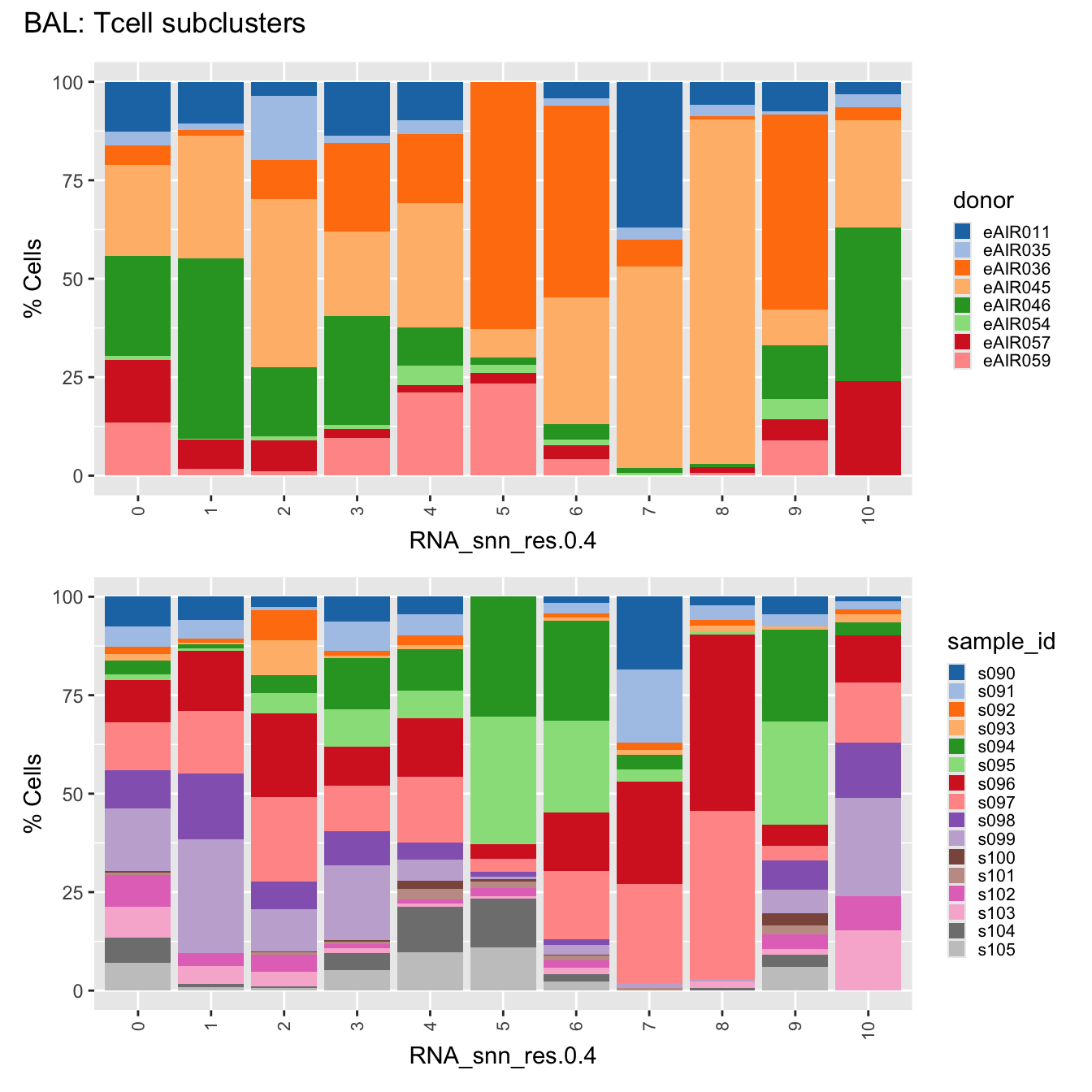
| Version | Author | Date |
|---|---|---|
| 6d2b67f | Gunjan Dixit | 2024-12-24 |
Updated cell-type labels (T cell clusters)
cell_labels <- readxl::read_excel(here("data/cell_labels_Mel_v4_Dec2024/earlyAIR_BAL_all.xlsx"), sheet = "T-reclustering")

new_cluster_names <- cell_labels %>%
  dplyr::select(cluster, annotation) %>%
  deframe()

paed_sub <- RenameIdents(paed_sub, new_cluster_names)
paed_sub@meta.data$cell_labels_v2 <- Idents(paed_sub)

p3 <- DimPlot(paed_sub, reduction = "umap.tcell", raster = FALSE, repel = TRUE, label = TRUE, label.size = 3.5) + ggtitle(paste0(tissue, ": UMAP with Updated T cell population"))

p3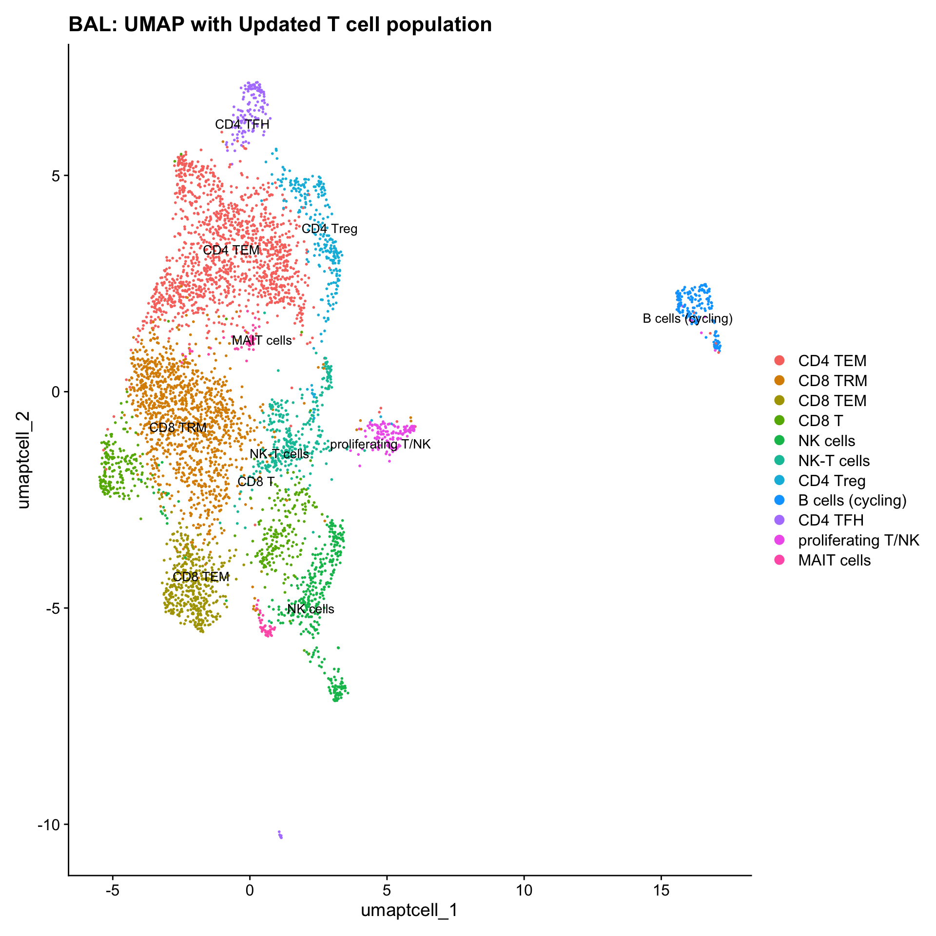
| Version | Author | Date |
|---|---|---|
| 6d2b67f | Gunjan Dixit | 2024-12-24 |
Reclustering B cells
Here is the link to marker gene analysis of B cells in BAL BAL_Bcell_res.0.4
idx <- which(Idents(seu_obj) %in% "B cells")
idx2 <- which(Idents(paed_sub) %in% "B cells (cycling)")
paed_bcells <- merge(seu_obj[,idx], paed_sub[,idx2])
paed_bcells
An object of class Seurat
17529 features across 1950 samples within 1 assay
Active assay: RNA (17529 features, 2000 variable features)
6 layers present: counts.1, counts.2, data.1, scale.data.1, data.2, scale.data.2Save subclustered SEU object (T cells labeled)
Save after removing B cells (cycling)
paed_sub <- paed_sub[,-idx2] # removing B cells from T cell subclusters
out2 <- here("output",
            "RDS", "AllBatches_Annotated_Subclustering_SEUs_v2", tissue,
             paste0("G000231_Neeland_",tissue,".Tcell_population.subclusters.SEU.rds"))
#dir.create(out2)
#if (!file.exists(out2)) {
  saveRDS(paed_sub, file = out2)
#}
Normalising B cell subclusters
paed_bcells <- paed_bcells %>%
NormalizeData() %>%
FindVariableFeatures() %>%
ScaleData() %>%
RunPCA()
Normalizing layer: counts.1Normalizing layer: counts.2Finding variable features for layer counts.1Finding variable features for layer counts.2Centering and scaling data matrixPC_ 1
Positive: CD44, TNFRSF13B, MPEG1, FCMR, CAPG, PTPN1, ITGAX, KLF2, PLEKHO1, ZEB2
LITAF, PARP15, ADGRE5, ACP5, ZFP36L2, CCR6, DUSP4, BANK1, ZFP36, SKI
SOCS3, TSC22D3, PLAC8, LY6E, CCDC50, EMP3, RIN3, PREX1, BHLHE40, NLRC5
Negative: NUGGC, MKI67, MEF2B, MYBL1, MYBL2, HMCES, TOP2A, STMN1, CDK1, HMGB2
HIST1H1B, TYMS, MARCKSL1, RGS13, SYNE2, CCNB2, FANCA, AURKB, ASF1B, HJURP
AFF2, KIF2C, BUB1, HIST1H2BH, TK1, GCSAM, TPX2, HIST1H4C, BCL6, CDCA7
PC_ 2
Positive: NIBAN3, TCL1A, IGHD, P2RX5, IGHM, DTX1, CD22, S1PR1, NEIL1, MARCKSL1
VPREB3, ALOX5, KLHL14, CRIP3, ELL3, TSPAN13, CR2, FCER2, BACH2, MEF2B
LARGE2, SATB1, PIK3IP1, BCL6, ARRDC3, CD38, SLC2A5, ISG20, FOXP1, BCL7A
Negative: ITGAX, CRIP1, FCRL4, VIM, DUSP4, IFI30, ADGRE5, TESC, KCTD12, ZBTB32
LIMK1, TNFRSF13B, PREX1, GSN, BHLHE40, PTPN1, FLNA, PFN1, LSP1, COTL1
NR4A1, SEMA7A, FOSL2, KLF6, CAPG, EFHD2, THEMIS2, ARID3A, IRF2BP2, ZYX
PC_ 3
Positive: MEF2B, KLHL6, CD27, DUSP2, SEMA4A, SERPINA9, FGD6, SPRED2, MYO1E, RAPGEF5
LOXL2, LMO2, SIAH2, RGS13, PTPRS, LHFPL2, CAMK1, P2RY12, MARCKSL1, CD83
CTSH, MAML3, CD40, SYNE2, LRMP, NLRP4, BCL2L11, TRAF4, NIBAN1, BCL6
Negative: TOP2A, PLK1, MKI67, AURKB, TPX2, CDCA8, HJURP, KIF2C, BUB1, CDC20
ASPM, CDK1, DLGAP5, HMMR, CENPA, CCNB2, CENPF, HIST1H1B, KIF23, AURKA
HIST1H2BH, CCNA2, NDC80, CCNB1, NEK2, IGHM, KIF20A, CEP55, UBE2C, CDCA2
PC_ 4
Positive: MYC, EGR3, NR4A3, NFKBID, NR4A1, KDM6B, DUSP2, PIM3, CD83, IRF4
EGR2, NR4A2, CCR7, SLCO4A1, HSP90AB1, NFKBIA, SLC7A5, JUNB, BCL2, SQSTM1
FOSL2, DUSP4, CDKN1A, GBP2, PPP1R15A, SLAMF7, NINJ1, SLC3A2, G0S2, EBI3
Negative: FCRL4, CD52, TLR10, TMSB4X, FCRL2, CCR6, PLD4, BHLHE41, FUT7, LTB
GSN, SMIM14, IFNGR1, SOX5, ITGB7, EVI2B, KCTD12, GAPT, GPR34, RESF1
ESYT1, SLC4A7, ACTG1, CCR1, CNN2, DDIT4, ACTB, ENTPD1, HHEX, ITGAX
PC_ 5
Positive: CCNB1, PLK1, CENPA, KIF20A, ASPM, CDC20, NEK2, DLGAP5, CENPF, HMMR
AURKA, KPNA2, GPSM2, ECT2, PSRC1, KNSTRN, KIF23, CENPE, CCNB2, ARHGAP11A
TPX2, UBE2C, PIF1, CKS2, CDCA8, SGO2, DEPDC1, NUGGC, KIF18A, HJURP
Negative: UHRF1, CDC45, MCM4, RRM2, CDT1, CDC6, PCLAF, E2F1, CCNE2, GINS2
DTL, MCM2, ASF1B, TYMS, MCM3, HELLS, RECQL4, POLE2, MCM6, TK1
FAM111B, TCF19, C19orf48, UNG, XRCC2, ATAD2, DONSON, WDR76, CTNNAL1, RFC2 paed_bcells <- RunUMAP(paed_bcells, dims = 1:30, reduction = "pca", reduction.name = "umap.bcell")11:30:54 UMAP embedding parameters a = 0.9922 b = 1.112Found more than one class "dist" in cache; using the first, from namespace 'spam'Also defined by 'BiocGenerics'11:30:54 Read 1950 rows and found 30 numeric columns11:30:54 Using Annoy for neighbor search, n_neighbors = 30Found more than one class "dist" in cache; using the first, from namespace 'spam'Also defined by 'BiocGenerics'11:30:54 Building Annoy index with metric = cosine, n_trees = 500% 10 20 30 40 50 60 70 80 90 100%[----|----|----|----|----|----|----|----|----|----|**************************************************|
11:30:54 Writing NN index file to temp file /var/folders/q8/kw1r78g12qn793xm7g0zvk94x2bh70/T//RtmpEQKiXk/file1623a00e822
11:30:54 Searching Annoy index using 1 thread, search_k = 3000
11:30:54 Annoy recall = 100%
11:30:55 Commencing smooth kNN distance calibration using 1 thread with target n_neighbors = 30
11:30:55 Initializing from normalized Laplacian + noise (using RSpectra)
11:30:55 Commencing optimization for 500 epochs, with 80016 positive edges
11:30:57 Optimization finishedmeta_data_columns <- colnames(paed_bcells@meta.data)
columns_to_remove <- grep("^RNA_snn_res", meta_data_columns, value = TRUE)
paed_bcells@meta.data <- paed_bcells@meta.data[, !(colnames(paed_bcells@meta.data) %in% columns_to_remove)]
resolutions <- seq(0.1, 1, by = 0.1)
paed_bcells <- FindNeighbors(paed_bcells, reduction = "pca", dims = 1:30)
paed_bcells <- FindClusters(paed_bcells, resolution = resolutions, algorithm = 3)Modularity Optimizer version 1.3.0 by Ludo Waltman and Nees Jan van Eck
Number of nodes: 1950
Number of edges: 81799
Running smart local moving algorithm...
Maximum modularity in 10 random starts: 0.9243
Number of communities: 2
Elapsed time: 0 seconds
Modularity Optimizer version 1.3.0 by Ludo Waltman and Nees Jan van Eck
Number of nodes: 1950
Number of edges: 81799
Running smart local moving algorithm...
Maximum modularity in 10 random starts: 0.8831
Number of communities: 4
Elapsed time: 0 seconds
Modularity Optimizer version 1.3.0 by Ludo Waltman and Nees Jan van Eck
Number of nodes: 1950
Number of edges: 81799
Running smart local moving algorithm...
Maximum modularity in 10 random starts: 0.8511
Number of communities: 4
Elapsed time: 0 seconds
Modularity Optimizer version 1.3.0 by Ludo Waltman and Nees Jan van Eck
Number of nodes: 1950
Number of edges: 81799
Running smart local moving algorithm...
Maximum modularity in 10 random starts: 0.8267
Number of communities: 5
Elapsed time: 0 seconds
Modularity Optimizer version 1.3.0 by Ludo Waltman and Nees Jan van Eck
Number of nodes: 1950
Number of edges: 81799
Running smart local moving algorithm...
Maximum modularity in 10 random starts: 0.8046
Number of communities: 5
Elapsed time: 0 seconds
Modularity Optimizer version 1.3.0 by Ludo Waltman and Nees Jan van Eck
Number of nodes: 1950
Number of edges: 81799
Running smart local moving algorithm...
Maximum modularity in 10 random starts: 0.7814
Number of communities: 5
Elapsed time: 0 seconds
Modularity Optimizer version 1.3.0 by Ludo Waltman and Nees Jan van Eck
Number of nodes: 1950
Number of edges: 81799
Running smart local moving algorithm...
Maximum modularity in 10 random starts: 0.7609
Number of communities: 6
Elapsed time: 0 seconds
Modularity Optimizer version 1.3.0 by Ludo Waltman and Nees Jan van Eck
Number of nodes: 1950
Number of edges: 81799
Running smart local moving algorithm...
Maximum modularity in 10 random starts: 0.7430
Number of communities: 7
Elapsed time: 0 seconds
Modularity Optimizer version 1.3.0 by Ludo Waltman and Nees Jan van Eck
Number of nodes: 1950
Number of edges: 81799
Running smart local moving algorithm...
Maximum modularity in 10 random starts: 0.7268
Number of communities: 8
Elapsed time: 0 seconds
Modularity Optimizer version 1.3.0 by Ludo Waltman and Nees Jan van Eck
Number of nodes: 1950
Number of edges: 81799
Running smart local moving algorithm...
Maximum modularity in 10 random starts: 0.7124
Number of communities: 10
Elapsed time: 0 secondsDimHeatmap(paed_bcells, dims = 1:10, cells = 500, balanced = TRUE)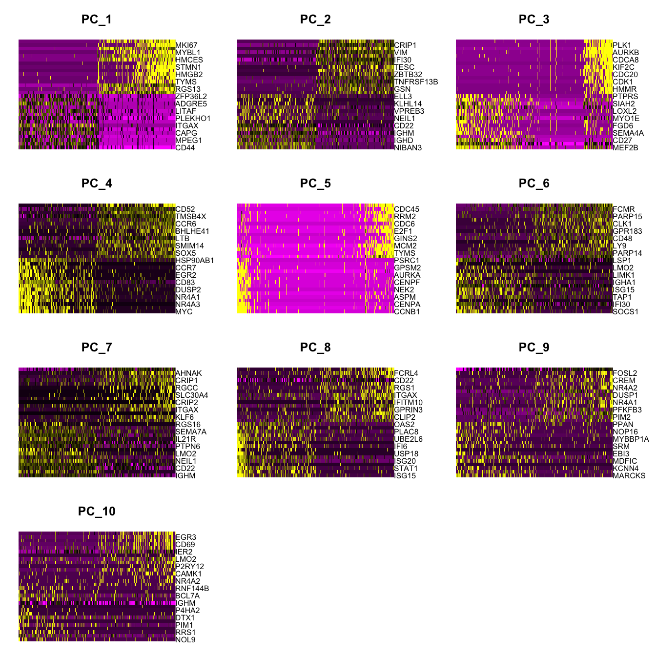
clustree(paed_bcells, prefix = "RNA_snn_res.")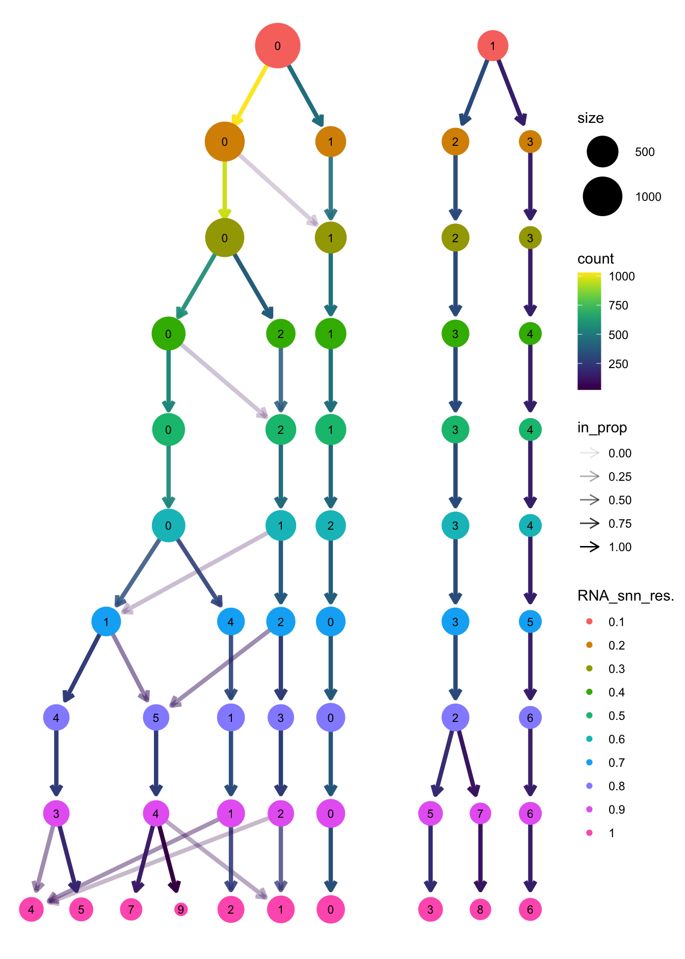
opt_res <- "RNA_snn_res.0.4"
n <- nlevels(paed_bcells$RNA_snn_res.0.4)
paed_bcells$RNA_snn_res.0.4 <- factor(paed_bcells$RNA_snn_res.0.4, levels = seq(0,n-1))
paed_bcells$seurat_clusters <- NULL
Idents(paed_bcells) <- paed_bcells$RNA_snn_res.0.4
DimPlot(paed_bcells, reduction = "umap.bcell", group.by = "RNA_snn_res.0.4", label = TRUE, label.size = 4.5, repel = TRUE, raster = FALSE )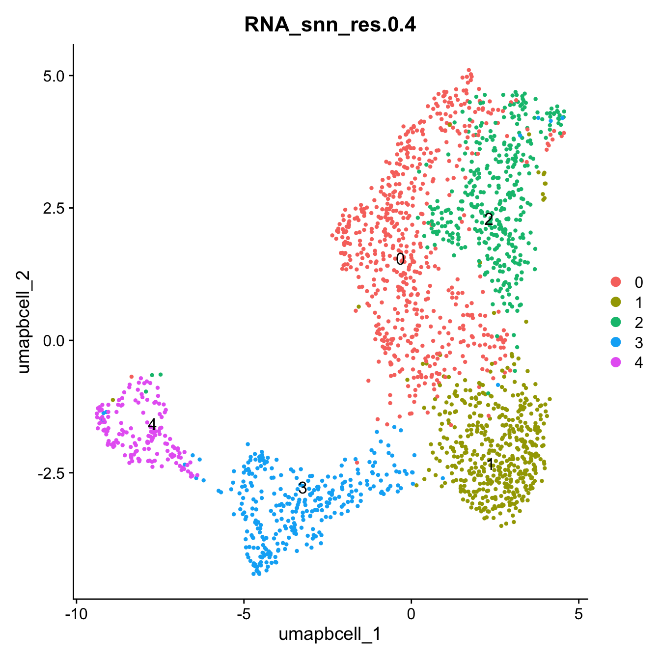
paed_bcells <- JoinLayers(paed_bcells)
paed_bcells.markers <- FindAllMarkers(paed_bcells, only.pos = TRUE, min.pct = 0.25, logfc.threshold = 0.25)
Calculating cluster 0Calculating cluster 1Calculating cluster 2Calculating cluster 3Calculating cluster 4paed_bcells.markers %>%
group_by(cluster) %>% unique() %>%
top_n(n = 5, wt = avg_log2FC) -> top5
paed_bcells.markers %>%
group_by(cluster) %>%
slice_head(n=1) %>%
pull(gene) -> best.wilcox.gene.per.cluster
best.wilcox.gene.per.cluster[1] "ITGAX" "IGHD" "MT-ND6" "MEF2B" "KIFC1" FeaturePlot(paed_bcells,features=best.wilcox.gene.per.cluster, reduction="umap.bcell",raster = FALSE, label = T, ncol = 3)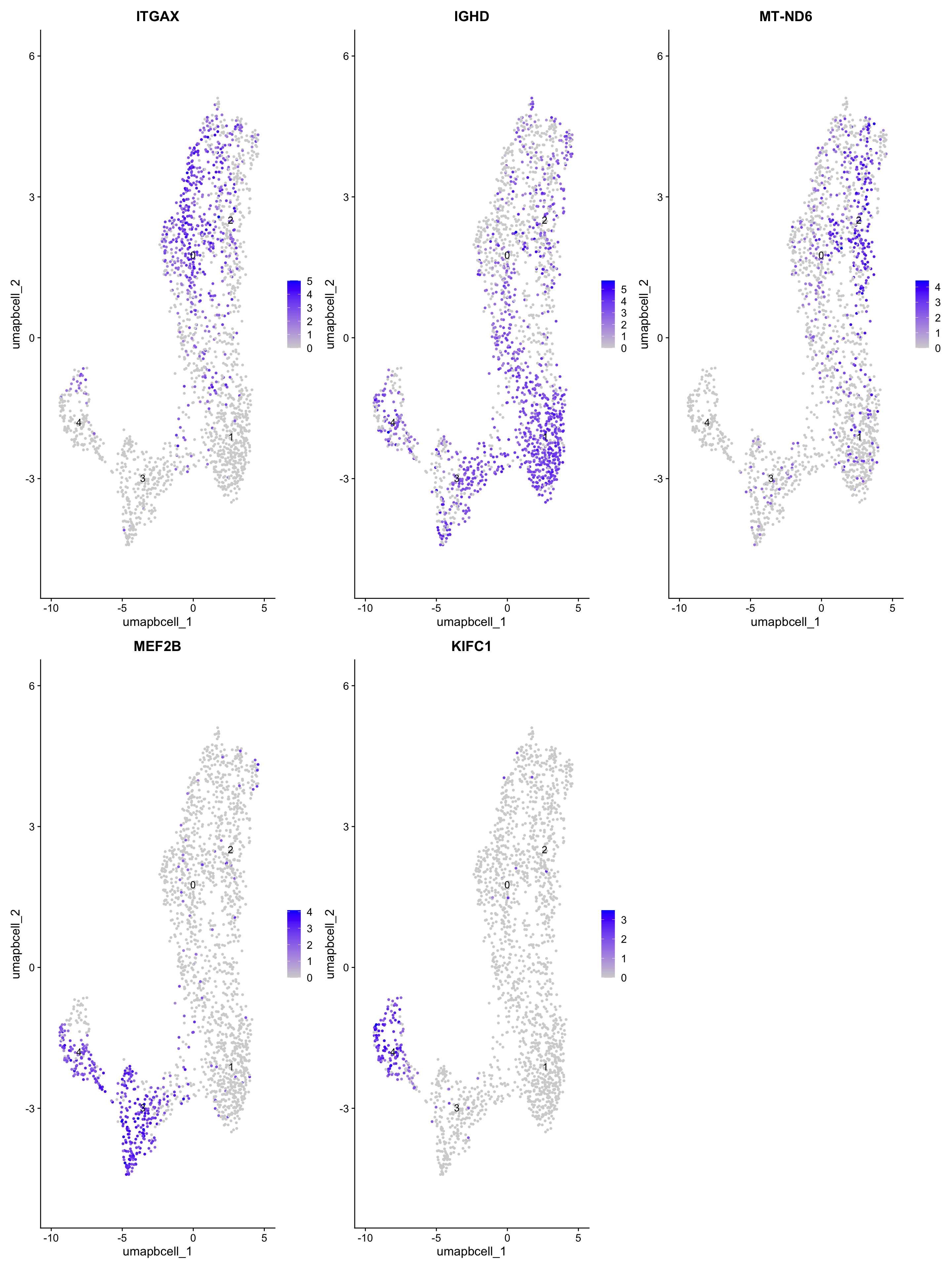
Top 10 marker genes from Seurat
## Seurat top markers
top10 <- paed_bcells.markers %>%
    group_by(cluster) %>%
    top_n(n = 10, wt = avg_log2FC) %>%
    ungroup() %>%
    distinct(gene, .keep_all = TRUE) %>%
    arrange(cluster, desc(avg_log2FC))

cluster_colors <- paletteer::paletteer_d("pals::glasbey")[factor(top10$cluster)]

DotPlot(paed_bcells,
        features = unique(top10$gene),
        group.by = opt_res,
        cols = c("azure1", "blueviolet"),
        dot.scale = 3, assay = "RNA") +
    RotatedAxis() +
    FontSize(y.text = 8, x.text = 12) +
    labs(y = element_blank(), x = element_blank()) +
    coord_flip() +
    theme(axis.text.y = element_text(color = cluster_colors)) +
    ggtitle("Top 10 marker genes per cluster (Seurat)")
Warning: Vectorized input to `element_text()` is not officially supported.
ℹ Results may be unexpected or may change in future versions of ggplot2.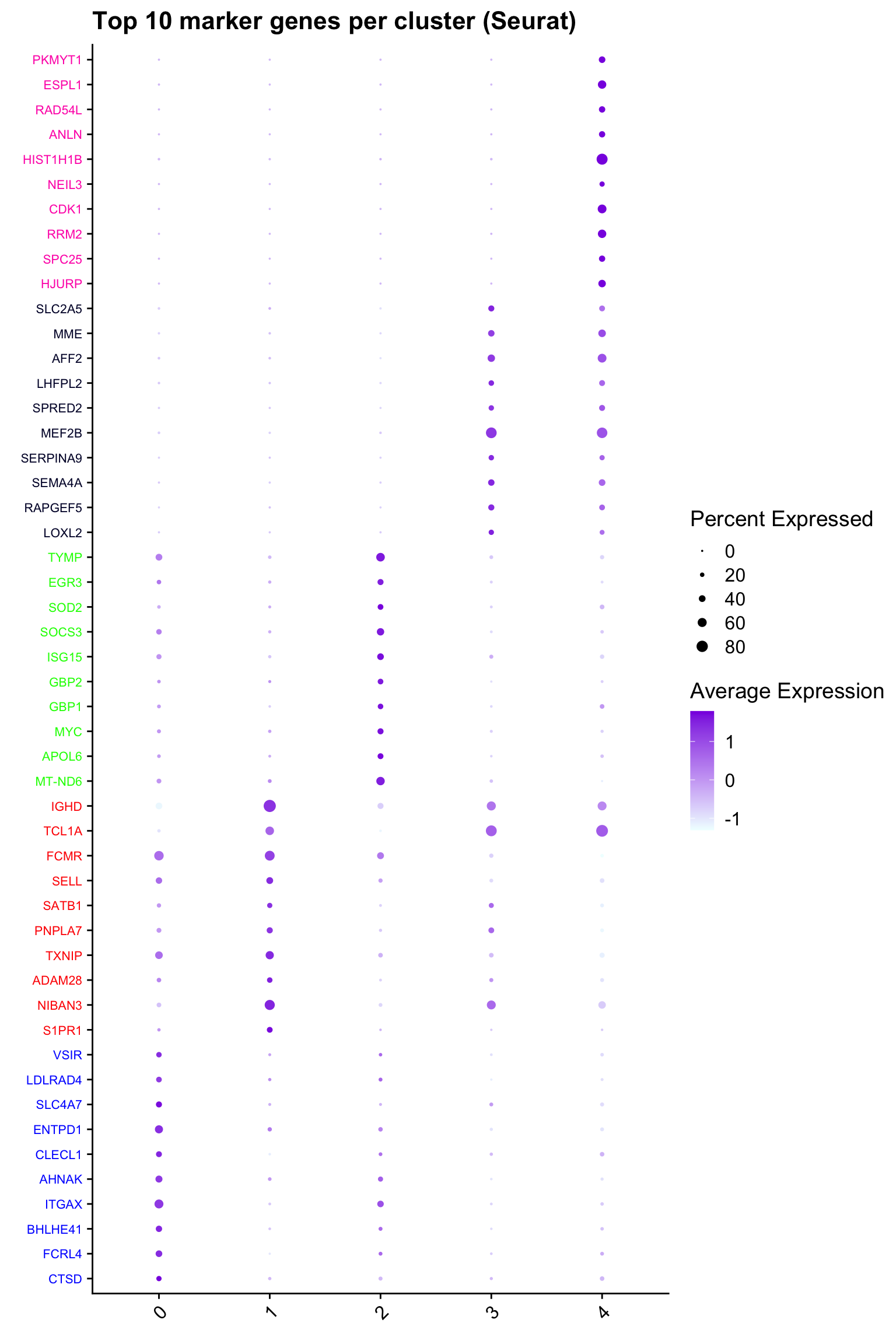
| Version | Author | Date |
|---|---|---|
| 74a78f0 | Gunjan Dixit | 2024-12-24 |
out_markers <- here("output",
            "CSV_v2",tissue,
            paste(tissue,"_Marker_genes_Reclustered_Bcell_population.",opt_res, sep = ""))

dir.create(out_markers, recursive = TRUE, showWarnings = FALSE)

for (cl in unique(paed_bcells.markers$cluster)) {
  cluster_data <- paed_bcells.markers %>% dplyr::filter(cluster == cl)
  file_name <- here(out_markers, paste0("G000231_Neeland_",tissue, "_cluster_", cl, ".csv"))
  if (!file.exists(file_name)) {
  write.csv(cluster_data, file = file_name)
  }
}
Updated cell-type labels (B cell clusters)
cell_labels <- readxl::read_excel(here("data/cell_labels_Mel_v4_Dec2024/earlyAIR_BAL_all.xlsx"), sheet = "B-reclustering")

new_cluster_names <- cell_labels %>%
  dplyr::select(cluster, annotation) %>%
  deframe()

paed_bcells <- RenameIdents(paed_bcells, new_cluster_names)
paed_bcells@meta.data$cell_labels_v2 <- Idents(paed_bcells)

p3 <- DimPlot(paed_bcells, reduction = "umap.bcell", raster = FALSE, repel = TRUE, label = TRUE, label.size = 3.5) + ggtitle(paste0(tissue, ": UMAP with Updated B cell population"))

p3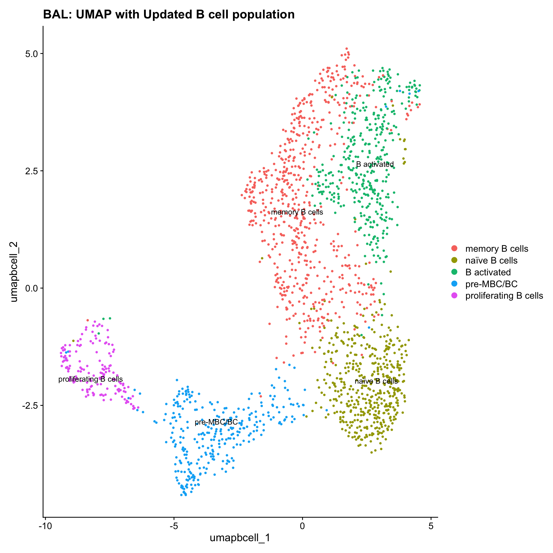
Save subclustered SEU object Bcells
out2 <- here("output",
            "RDS", "AllBatches_Annotated_Subclustering_SEUs_v2", tissue,
             paste0("G000231_Neeland_",tissue,".Bcell_population.subclusters.SEU.rds"))
#dir.create(out2)
#if (!file.exists(out2)) {
  saveRDS(paed_bcells, file = out2)
#}
Other Clusters (excluding subclusters)
idx <- which(Idents(seu_obj) %in% c("T cells for reclustering", "B cells"))
paed_other <- seu_obj[,-idx]
paed_other
An object of class Seurat
17529 features across 44948 samples within 1 assay
Active assay: RNA (17529 features, 2000 variable features)
3 layers present: counts, data, scale.data
2 dimensional reductions calculated: pca, umapSave subclustered SEU object ( All other cells)
paed_other$cell_labels_v2 <-paed_other$cell_labels
out2 <- here("output",
            "RDS", "AllBatches_Annotated_Subclustering_SEUs_v2", tissue,
             paste0("G000231_Neeland_",tissue,".all_other.subclusters.SEU.rds"))
#dir.create(out2)
#if (!file.exists(out2)) {
  saveRDS(paed_other, file = out2)
#}
Merge seurat objects of subclusters
files <- list.files(here("output",
            "RDS", "AllBatches_Annotated_Subclustering_SEUs_v2", tissue),
                    full.names = TRUE)

seuLst <- lapply(files, function(f) readRDS(f))

seu <- merge(seuLst[[1]],
             y = c(seuLst[[2]],
                   seuLst[[3]]))
seu
An object of class Seurat
17529 features across 51604 samples within 1 assay
Active assay: RNA (17529 features, 2000 variable features)
11 layers present: counts.1, counts.2, counts.3, data.1, scale.data.1, data.2, scale.data.1.2, scale.data.2.2, scale.data.2, data.3, scale.data.3merged <- seu %>%
NormalizeData() %>%
FindVariableFeatures() %>%
ScaleData() %>%
RunPCA()Normalizing layer: counts.1Normalizing layer: counts.2Normalizing layer: counts.3Finding variable features for layer counts.1Finding variable features for layer counts.2Finding variable features for layer counts.3Centering and scaling data matrixPC_ 1
Positive: TPPP3, C9orf24, LRRC46, C20orf85, DNAAF1, LDLRAD1, FAM92B, FOXJ1, ZMYND10, SPATA18
MS4A8, SNTN, RSPH1, TEKT1, PROM1, CFAP43, TSPAN1, VWA3A, AC007906.2, SLC44A4
LRRC10B, CDHR3, CTXN1, ROPN1L, CFAP157, PIFO, DRC3, DNAH9, PTPRT, CAPS
Negative: VIM, TMSB4X, LCP1, SPI1, SRGN, IFI30, ALOX5, S100A4, MS4A7, OLR1
LGALS1, PFN1, LRP1, ADAMTSL4, SLC11A1, COTL1, MSR1, ACTB, CYBB, EMP3
VSIG4, HCK, FABP4, CD163, SLCO2B1, HK3, IRF8, OSCAR, PPARG, ZEB2
PC_ 2
Positive: TNFSF13, LRP1, MS4A7, MSR1, ALOX5, FABP4, ADAMTSL4, VIM, SPI1, VSIG4
OLR1, SLCO2B1, IFI30, CRIP1, SLC11A1, PPARG, C5AR1, CD4, S100A4, CTSH
OSCAR, LGALS1, CD163, KCTD12, CEBPB, MME, HK3, FN1, CYBB, CD9
Negative: KRT7, GABRP, F3, CEACAM6, PRSS8, AQP5, CEACAM5, KLK11, MSLN, LYPD2
CYP2F1, PRSS23, FAM3D, SCGB3A1, ALPL, FCGBP, UPK1B, KRT19, MSMB, SLC6A14
MUC1, GPRC5A, BPIFB1, MUC5B, ASS1, ATP12A, CXCL17, FUT3, SLC5A8, S100A16
PC_ 3
Positive: CEBPB, CD9, C5AR1, S100A9, OLR1, IFI30, HSPB1, GSN, LRP1, SLC11A1
MSR1, TNFSF13, LMNA, SPI1, ADAMTSL4, CD163, TYMP, HK3, MS4A7, ALOX5
RHOB, SLCO2B1, IFI6, EFHD2, SAT1, FABP4, VSIG4, HCK, OSCAR, KCTD12
Negative: MKI67, TYMS, HIST1H1B, KIFC1, TOP2A, MYBL2, CENPM, BIRC5, TRBC2, TPX2
RRM2, CDK1, FOXM1, LTB, SPC24, PCLAF, AURKB, ANLN, IL32, NCAPG
NUSAP1, CDCA5, TK1, HIST1H1D, PHF19, ASF1B, CD3E, PRC1, UHRF1, NDC80
PC_ 4
Positive: TYMS, MKI67, KIFC1, TOP2A, CDK1, TK1, RRM2, BIRC5, TPX2, ANLN
FOXM1, PCLAF, ASF1B, CDCA5, SPC24, CDT1, CEP55, ZWINT, NCAPG, STMN1
HIST1H1B, CCNB2, NUSAP1, PRC1, HJURP, TCF19, AURKB, KIF2C, CDKN2C, CD9
Negative: SERPINB9, SOCS3, IL4I1, TNFRSF1B, TRAF1, ZFP36, PFKFB3, NR4A3, IER3, CCL3
NINJ1, SPHK1, CCL4, TNFAIP3, DUSP2, CCR5, ADAM19, GPR183, ICAM1, RGS1
G0S2, STAB1, SLAMF7, JUNB, CXCR4, CCL4L2, IL32, TRBC2, NFKB2, ARL4C
PC_ 5
Positive: IER3, SOD2, SOCS3, CCL3, NFKBIA, NINJ1, DUSP1, ZFP36, NR4A1, NR4A3
ICAM1, IL1B, SPHK1, IL1RN, IL4I1, SAT1, MARCKS, GADD45B, ATF3, PPP1R15A
JUNB, G0S2, CCL4, PIM3, TIMP1, C15orf48, CXCL10, CDKN1A, PFKFB3, TNFAIP3
Negative: TRBC2, CD3E, IL32, CD96, IL2RB, CD8A, SPOCK2, CCL5, TRBC1, CD7
CXCR6, LTB, GZMA, ZNF683, CTSW, SYNE2, CRIP1, AQP3, PRF1, CCND3
SYTL1, LBH, TIGIT, C8B, RESF1, TMSB4X, TCF7, SLCO2B1, KLRD1, GRAP2 merged <- RunUMAP(merged, dims = 1:30, reduction = "pca", reduction.name = "umap.merged")11:34:42 UMAP embedding parameters a = 0.9922 b = 1.112Found more than one class "dist" in cache; using the first, from namespace 'spam'Also defined by 'BiocGenerics'11:34:42 Read 51604 rows and found 30 numeric columns11:34:42 Using Annoy for neighbor search, n_neighbors = 30Found more than one class "dist" in cache; using the first, from namespace 'spam'Also defined by 'BiocGenerics'11:34:42 Building Annoy index with metric = cosine, n_trees = 500% 10 20 30 40 50 60 70 80 90 100%[----|----|----|----|----|----|----|----|----|----|**************************************************|
11:34:44 Writing NN index file to temp file /var/folders/q8/kw1r78g12qn793xm7g0zvk94x2bh70/T//RtmpEQKiXk/file162312128d38
11:34:44 Searching Annoy index using 1 thread, search_k = 3000
11:34:54 Annoy recall = 100%
11:34:54 Commencing smooth kNN distance calibration using 1 thread with target n_neighbors = 30
11:34:55 Found 2 connected components, falling back to 'spca' initialization with init_sdev = 1
Found more than one class "dist" in cache; using the first, from namespace 'spam'
Also defined by 'BiocGenerics'
11:34:55 Using 'irlba' for PCA
11:34:56 PCA: 2 components explained 55.07% variance
11:34:56 Scaling init to sdev = 1
11:34:56 Commencing optimization for 200 epochs, with 2243846 positive edges
11:35:10 Optimization finishedp4 <- DimPlot(merged, reduction = "umap.merged", group.by = "cell_labels_v2",raster = FALSE, repel = TRUE, label = TRUE, label.size = 4.5) + ggtitle(paste0(tissue, ": UMAP with annotations")) + NoLegend()
p4Warning: ggrepel: 1 unlabeled data points (too many overlaps). Consider
increasing max.overlaps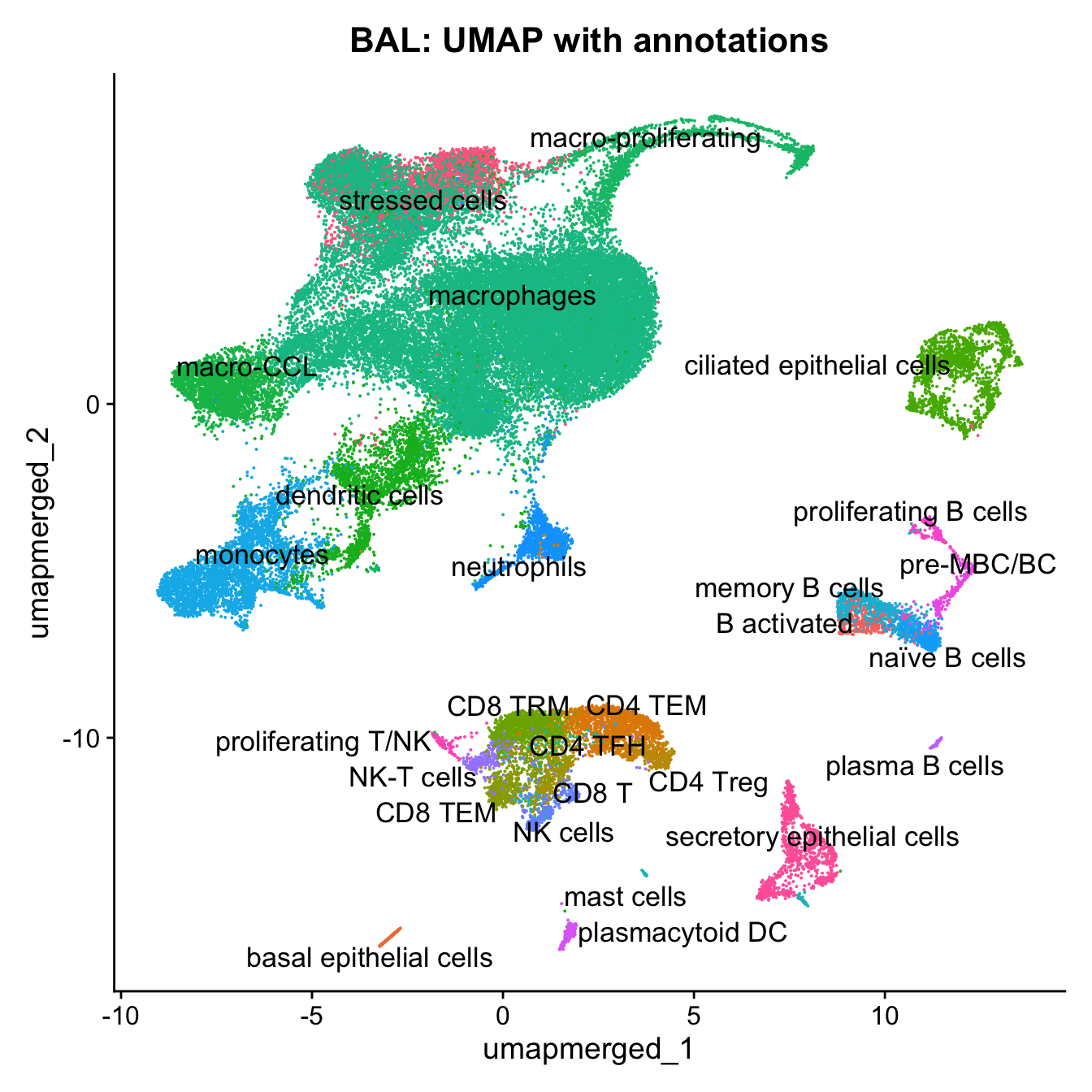
labels <- c( "predicted.ann_level_3", "predicted.ann_level_4", "predicted.ann_finest_level", "cell_labels","cell_labels_v2")

p <- vector("list",length(labels))
for(label in labels){
  merged@meta.data %>%
    ggplot(aes(x = !!sym(label),
               fill = !!sym(label))) +
    geom_bar() +
    geom_text(aes(label = ..count..), stat = "count",
              vjust = -0.5, colour = "black", size = 2) +
    scale_y_log10() +
    theme(axis.text.x = element_blank(),
          axis.title.x = element_blank(),
          axis.ticks.x = element_blank()) +
    NoLegend() +
    labs(y = "No. Cells (log scale)") -> p1

  merged@meta.data %>%
    dplyr::select(!!sym(label), donor) %>%
    group_by(!!sym(label), donor) %>%
    summarise(num = n()) %>%
    mutate(prop = num / sum(num)) %>%
  ggplot(aes(x = !!sym(label), y = prop * 100,
             fill = donor)) +
    geom_bar(stat = "identity") +
    theme(axis.text.x = element_text(angle = 90,
                                     vjust = 0.5,
                                     hjust = 1,
                                     size = 8)) +
    labs(y = "% Cells", fill = "Donor") +
  scale_fill_manual(values = combined_palette) -> p2

  (p1 / p2) & theme(legend.text = element_text(size = 8),
                  legend.key.size = unit(3, "mm")) -> p[[label]]
}
`summarise()` has grouped output by 'predicted.ann_level_3'. You can override
using the `.groups` argument.
`summarise()` has grouped output by 'predicted.ann_level_4'. You can override
using the `.groups` argument.
`summarise()` has grouped output by 'predicted.ann_finest_level'. You can
override using the `.groups` argument.
`summarise()` has grouped output by 'cell_labels'. You can override using the
`.groups` argument.
`summarise()` has grouped output by 'cell_labels_v2'. You can override using
the `.groups` argument.p[[1]]
NULL
[[2]]
NULL
[[3]]
NULL
[[4]]
NULL
[[5]]
NULL
$predicted.ann_level_3
| Version | Author | Date |
|---|---|---|
| 54e4ec2 | Gunjan Dixit | 2025-01-08 |
$predicted.ann_level_4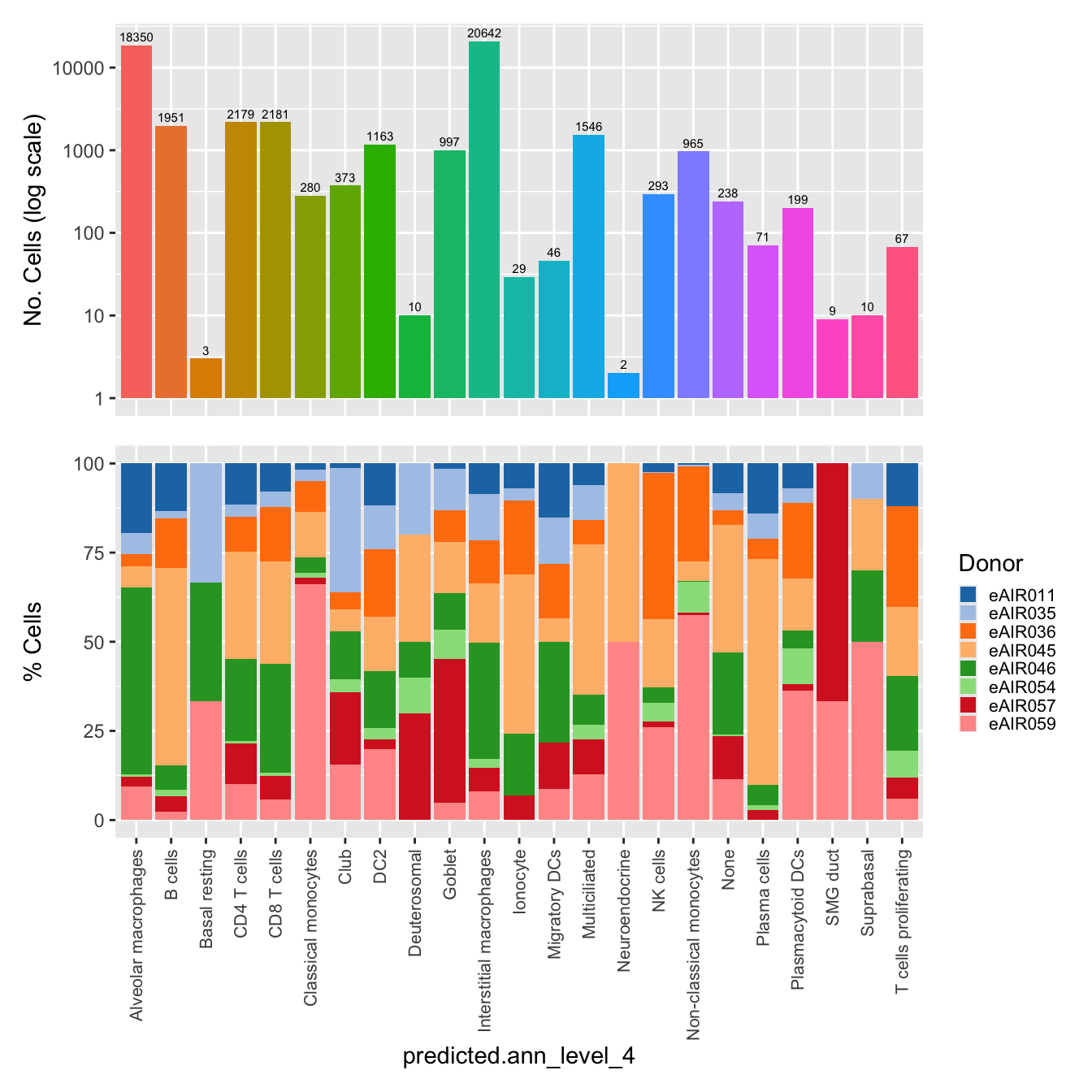
$predicted.ann_finest_level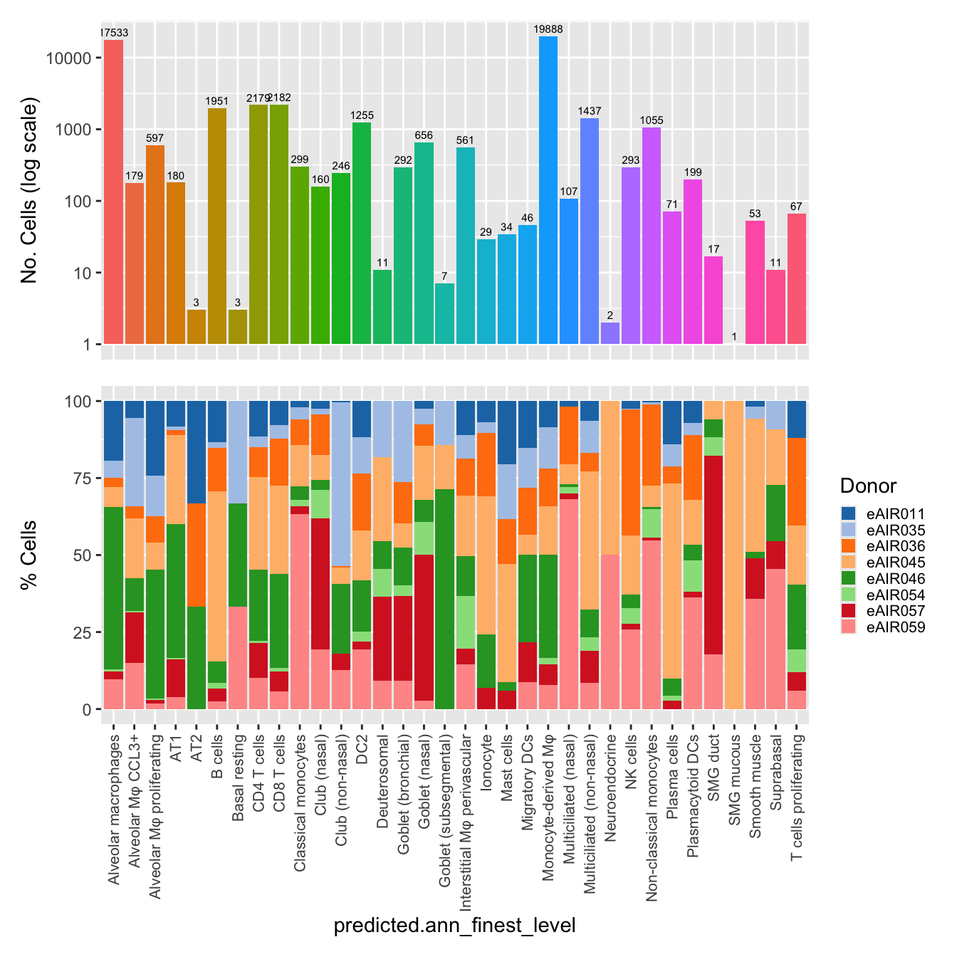
$cell_labels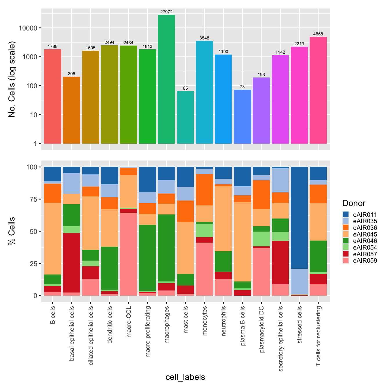
$cell_labels_v2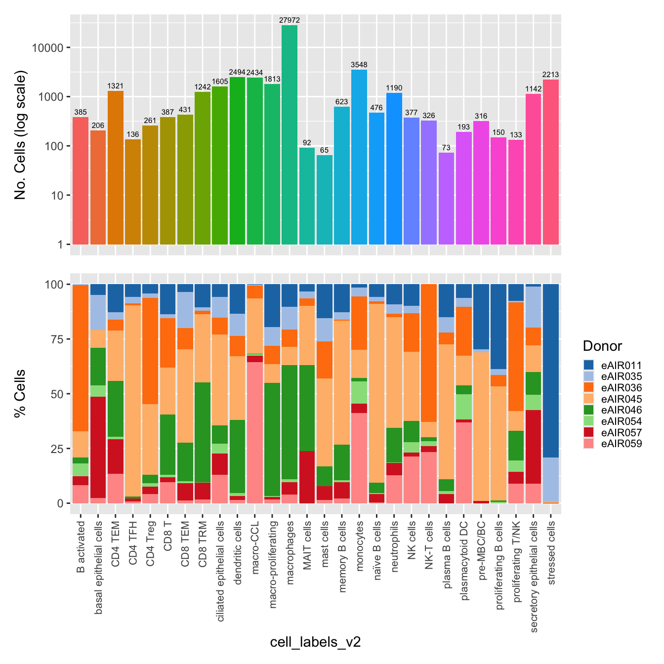
Save Final SEU object (All cells)
out3 <- here("output",
            "RDS", "AllBatches_Final_Clusters_SEUs_v2",
             paste0("G000231_Neeland_",tissue,".final_clusters.SEU.rds"))

if (!file.exists(out3)) {
  saveRDS(merged, file = out3)
}
Session Info
sessioninfo::session_info()─ Session info ───────────────────────────────────────────────────────────────
setting value
version R version 4.3.2 (2023-10-31)
os macOS 15.2
system aarch64, darwin20
ui X11
language (EN)
collate en_US.UTF-8
ctype en_US.UTF-8
tz Australia/Melbourne
date 2025-01-16
pandoc 3.1.1 @ /Users/dixitgunjan/Desktop/RStudio.app/Contents/Resources/app/quarto/bin/tools/ (via rmarkdown)
─ Packages ───────────────────────────────────────────────────────────────────
package * version date (UTC) lib source
abind 1.4-5 2016-07-21 [1] CRAN (R 4.3.0)
AnnotationDbi * 1.64.1 2023-11-02 [1] Bioconductor
backports 1.4.1 2021-12-13 [1] CRAN (R 4.3.0)
beeswarm 0.4.0 2021-06-01 [1] CRAN (R 4.3.0)
Biobase * 2.62.0 2023-10-26 [1] Bioconductor
BiocGenerics * 0.48.1 2023-11-02 [1] Bioconductor
BiocManager 1.30.22 2023-08-08 [1] CRAN (R 4.3.0)
BiocStyle * 2.30.0 2023-10-26 [1] Bioconductor
Biostrings 2.70.2 2024-01-30 [1] Bioconductor 3.18 (R 4.3.2)
bit 4.0.5 2022-11-15 [1] CRAN (R 4.3.0)
bit64 4.0.5 2020-08-30 [1] CRAN (R 4.3.0)
bitops 1.0-7 2021-04-24 [1] CRAN (R 4.3.0)
blob 1.2.4 2023-03-17 [1] CRAN (R 4.3.0)
bslib 0.6.1 2023-11-28 [1] CRAN (R 4.3.1)
cachem 1.0.8 2023-05-01 [1] CRAN (R 4.3.0)
callr 3.7.5 2024-02-19 [1] CRAN (R 4.3.1)
cellranger 1.1.0 2016-07-27 [1] CRAN (R 4.3.0)
checkmate 2.3.1 2023-12-04 [1] CRAN (R 4.3.1)
cli 3.6.2 2023-12-11 [1] CRAN (R 4.3.1)
cluster 2.1.6 2023-12-01 [1] CRAN (R 4.3.1)
clustree * 0.5.1 2023-11-05 [1] CRAN (R 4.3.1)
codetools 0.2-19 2023-02-01 [1] CRAN (R 4.3.2)
colorspace 2.1-0 2023-01-23 [1] CRAN (R 4.3.0)
cowplot 1.1.3 2024-01-22 [1] CRAN (R 4.3.1)
crayon 1.5.2 2022-09-29 [1] CRAN (R 4.3.0)
data.table * 1.15.0 2024-01-30 [1] CRAN (R 4.3.1)
DBI 1.2.2 2024-02-16 [1] CRAN (R 4.3.1)
DelayedArray 0.28.0 2023-11-06 [1] Bioconductor
deldir 2.0-2 2023-11-23 [1] CRAN (R 4.3.1)
digest 0.6.34 2024-01-11 [1] CRAN (R 4.3.1)
dotCall64 1.1-1 2023-11-28 [1] CRAN (R 4.3.1)
dplyr * 1.1.4 2023-11-17 [1] CRAN (R 4.3.1)
edgeR * 4.0.16 2024-02-20 [1] Bioconductor 3.18 (R 4.3.2)
ellipsis 0.3.2 2021-04-29 [1] CRAN (R 4.3.0)
evaluate 0.23 2023-11-01 [1] CRAN (R 4.3.1)
fansi 1.0.6 2023-12-08 [1] CRAN (R 4.3.1)
farver 2.1.1 2022-07-06 [1] CRAN (R 4.3.0)
fastDummies 1.7.3 2023-07-06 [1] CRAN (R 4.3.0)
fastmap 1.1.1 2023-02-24 [1] CRAN (R 4.3.0)
fitdistrplus 1.1-11 2023-04-25 [1] CRAN (R 4.3.0)
forcats * 1.0.0 2023-01-29 [1] CRAN (R 4.3.0)
fs 1.6.3 2023-07-20 [1] CRAN (R 4.3.0)
future 1.33.1 2023-12-22 [1] CRAN (R 4.3.1)
future.apply 1.11.1 2023-12-21 [1] CRAN (R 4.3.1)
generics 0.1.3 2022-07-05 [1] CRAN (R 4.3.0)
GenomeInfoDb 1.38.6 2024-02-10 [1] Bioconductor 3.18 (R 4.3.2)
GenomeInfoDbData 1.2.11 2024-02-27 [1] Bioconductor
GenomicRanges 1.54.1 2023-10-30 [1] Bioconductor
getPass 0.2-4 2023-12-10 [1] CRAN (R 4.3.1)
ggbeeswarm 0.7.2 2023-04-29 [1] CRAN (R 4.3.0)
ggforce 0.4.2 2024-02-19 [1] CRAN (R 4.3.1)
ggplot2 * 3.5.0 2024-02-23 [1] CRAN (R 4.3.1)
ggraph * 2.1.0 2022-10-09 [1] CRAN (R 4.3.0)
ggrastr 1.0.2 2023-06-01 [1] CRAN (R 4.3.0)
ggrepel 0.9.5 2024-01-10 [1] CRAN (R 4.3.1)
ggridges 0.5.6 2024-01-23 [1] CRAN (R 4.3.1)
git2r 0.33.0 2023-11-26 [1] CRAN (R 4.3.1)
globals 0.16.2 2022-11-21 [1] CRAN (R 4.3.0)
glue * 1.7.0 2024-01-09 [1] CRAN (R 4.3.1)
goftest 1.2-3 2021-10-07 [1] CRAN (R 4.3.0)
graphlayouts 1.1.0 2024-01-19 [1] CRAN (R 4.3.1)
gridExtra 2.3 2017-09-09 [1] CRAN (R 4.3.0)
gtable 0.3.4 2023-08-21 [1] CRAN (R 4.3.0)
here * 1.0.1 2020-12-13 [1] CRAN (R 4.3.0)
highr 0.10 2022-12-22 [1] CRAN (R 4.3.0)
hms 1.1.3 2023-03-21 [1] CRAN (R 4.3.0)
htmltools 0.5.7 2023-11-03 [1] CRAN (R 4.3.1)
htmlwidgets 1.6.4 2023-12-06 [1] CRAN (R 4.3.1)
httpuv 1.6.14 2024-01-26 [1] CRAN (R 4.3.1)
httr 1.4.7 2023-08-15 [1] CRAN (R 4.3.0)
ica 1.0-3 2022-07-08 [1] CRAN (R 4.3.0)
igraph 2.0.2 2024-02-17 [1] CRAN (R 4.3.1)
IRanges * 2.36.0 2023-10-26 [1] Bioconductor
irlba 2.3.5.1 2022-10-03 [1] CRAN (R 4.3.2)
jquerylib 0.1.4 2021-04-26 [1] CRAN (R 4.3.0)
jsonlite 1.8.8 2023-12-04 [1] CRAN (R 4.3.1)
kableExtra * 1.4.0 2024-01-24 [1] CRAN (R 4.3.1)
KEGGREST 1.42.0 2023-10-26 [1] Bioconductor
KernSmooth 2.23-22 2023-07-10 [1] CRAN (R 4.3.2)
knitr 1.45 2023-10-30 [1] CRAN (R 4.3.1)
labeling 0.4.3 2023-08-29 [1] CRAN (R 4.3.0)
later 1.3.2 2023-12-06 [1] CRAN (R 4.3.1)
lattice 0.22-5 2023-10-24 [1] CRAN (R 4.3.1)
lazyeval 0.2.2 2019-03-15 [1] CRAN (R 4.3.0)
leiden 0.4.3.1 2023-11-17 [1] CRAN (R 4.3.1)
lifecycle 1.0.4 2023-11-07 [1] CRAN (R 4.3.1)
limma * 3.58.1 2023-11-02 [1] Bioconductor
listenv 0.9.1 2024-01-29 [1] CRAN (R 4.3.1)
lmtest 0.9-40 2022-03-21 [1] CRAN (R 4.3.0)
locfit 1.5-9.8 2023-06-11 [1] CRAN (R 4.3.0)
lubridate * 1.9.3 2023-09-27 [1] CRAN (R 4.3.1)
magrittr 2.0.3 2022-03-30 [1] CRAN (R 4.3.0)
MASS 7.3-60.0.1 2024-01-13 [1] CRAN (R 4.3.1)
Matrix 1.6-5 2024-01-11 [1] CRAN (R 4.3.1)
MatrixGenerics 1.14.0 2023-10-26 [1] Bioconductor
matrixStats 1.2.0 2023-12-11 [1] CRAN (R 4.3.1)
memoise 2.0.1 2021-11-26 [1] CRAN (R 4.3.0)
mime 0.12 2021-09-28 [1] CRAN (R 4.3.0)
miniUI 0.1.1.1 2018-05-18 [1] CRAN (R 4.3.0)
munsell 0.5.0 2018-06-12 [1] CRAN (R 4.3.0)
nlme 3.1-164 2023-11-27 [1] CRAN (R 4.3.1)
org.Hs.eg.db * 3.18.0 2024-02-27 [1] Bioconductor
paletteer 1.6.0 2024-01-21 [1] CRAN (R 4.3.1)
parallelly 1.37.0 2024-02-14 [1] CRAN (R 4.3.1)
patchwork * 1.2.0 2024-01-08 [1] CRAN (R 4.3.1)
pbapply 1.7-2 2023-06-27 [1] CRAN (R 4.3.0)
pillar 1.9.0 2023-03-22 [1] CRAN (R 4.3.0)
pkgconfig 2.0.3 2019-09-22 [1] CRAN (R 4.3.0)
plotly 4.10.4 2024-01-13 [1] CRAN (R 4.3.1)
plyr 1.8.9 2023-10-02 [1] CRAN (R 4.3.1)
png 0.1-8 2022-11-29 [1] CRAN (R 4.3.0)
polyclip 1.10-6 2023-09-27 [1] CRAN (R 4.3.1)
presto 1.0.0 2024-02-27 [1] Github (immunogenomics/presto@31dc97f)
prismatic 1.1.1 2022-08-15 [1] CRAN (R 4.3.0)
processx 3.8.3 2023-12-10 [1] CRAN (R 4.3.1)
progressr 0.14.0 2023-08-10 [1] CRAN (R 4.3.0)
promises 1.2.1 2023-08-10 [1] CRAN (R 4.3.0)
ps 1.7.6 2024-01-18 [1] CRAN (R 4.3.1)
purrr * 1.0.2 2023-08-10 [1] CRAN (R 4.3.0)
R6 2.5.1 2021-08-19 [1] CRAN (R 4.3.0)
RANN 2.6.1 2019-01-08 [1] CRAN (R 4.3.0)
RColorBrewer * 1.1-3 2022-04-03 [1] CRAN (R 4.3.0)
Rcpp 1.0.12 2024-01-09 [1] CRAN (R 4.3.1)
RcppAnnoy 0.0.22 2024-01-23 [1] CRAN (R 4.3.1)
RcppHNSW 0.6.0 2024-02-04 [1] CRAN (R 4.3.1)
RCurl 1.98-1.14 2024-01-09 [1] CRAN (R 4.3.1)
readr * 2.1.5 2024-01-10 [1] CRAN (R 4.3.1)
readxl * 1.4.3 2023-07-06 [1] CRAN (R 4.3.0)
rematch2 2.1.2 2020-05-01 [1] CRAN (R 4.3.0)
reshape2 1.4.4 2020-04-09 [1] CRAN (R 4.3.0)
reticulate 1.35.0 2024-01-31 [1] CRAN (R 4.3.1)
rlang 1.1.3 2024-01-10 [1] CRAN (R 4.3.1)
rmarkdown 2.25 2023-09-18 [1] CRAN (R 4.3.1)
ROCR 1.0-11 2020-05-02 [1] CRAN (R 4.3.0)
rprojroot 2.0.4 2023-11-05 [1] CRAN (R 4.3.1)
RSpectra 0.16-1 2022-04-24 [1] CRAN (R 4.3.0)
RSQLite 2.3.5 2024-01-21 [1] CRAN (R 4.3.1)
rstudioapi 0.15.0 2023-07-07 [1] CRAN (R 4.3.0)
Rtsne 0.17 2023-12-07 [1] CRAN (R 4.3.1)
S4Arrays 1.2.0 2023-10-26 [1] Bioconductor
S4Vectors * 0.40.2 2023-11-25 [1] Bioconductor 3.18 (R 4.3.2)
sass 0.4.8 2023-12-06 [1] CRAN (R 4.3.1)
scales 1.3.0 2023-11-28 [1] CRAN (R 4.3.1)
scattermore 1.2 2023-06-12 [1] CRAN (R 4.3.0)
sctransform 0.4.1 2023-10-19 [1] CRAN (R 4.3.1)
sessioninfo 1.2.2 2021-12-06 [1] CRAN (R 4.3.0)
Seurat * 5.0.1.9009 2024-02-28 [1] Github (satijalab/seurat@6a3ef5e)
SeuratObject * 5.0.1 2023-11-17 [1] CRAN (R 4.3.1)
shiny 1.8.0 2023-11-17 [1] CRAN (R 4.3.1)
SingleCellExperiment 1.24.0 2023-11-06 [1] Bioconductor
sp * 2.1-3 2024-01-30 [1] CRAN (R 4.3.1)
spam 2.10-0 2023-10-23 [1] CRAN (R 4.3.1)
SparseArray 1.2.4 2024-02-10 [1] Bioconductor 3.18 (R 4.3.2)
spatstat.data 3.0-4 2024-01-15 [1] CRAN (R 4.3.1)
spatstat.explore 3.2-6 2024-02-01 [1] CRAN (R 4.3.1)
spatstat.geom 3.2-8 2024-01-26 [1] CRAN (R 4.3.1)
spatstat.random 3.2-2 2023-11-29 [1] CRAN (R 4.3.1)
spatstat.sparse 3.0-3 2023-10-24 [1] CRAN (R 4.3.1)
spatstat.utils 3.0-4 2023-10-24 [1] CRAN (R 4.3.1)
speckle * 1.2.0 2023-10-26 [1] Bioconductor
statmod 1.5.0 2023-01-06 [1] CRAN (R 4.3.0)
stringi 1.8.3 2023-12-11 [1] CRAN (R 4.3.1)
stringr * 1.5.1 2023-11-14 [1] CRAN (R 4.3.1)
SummarizedExperiment 1.32.0 2023-11-06 [1] Bioconductor
survival 3.5-8 2024-02-14 [1] CRAN (R 4.3.1)
svglite 2.1.3 2023-12-08 [1] CRAN (R 4.3.1)
systemfonts 1.0.5 2023-10-09 [1] CRAN (R 4.3.1)
tensor 1.5 2012-05-05 [1] CRAN (R 4.3.0)
tibble * 3.2.1 2023-03-20 [1] CRAN (R 4.3.0)
tidygraph 1.3.1 2024-01-30 [1] CRAN (R 4.3.1)
tidyr * 1.3.1 2024-01-24 [1] CRAN (R 4.3.1)
tidyselect 1.2.0 2022-10-10 [1] CRAN (R 4.3.0)
tidyverse * 2.0.0 2023-02-22 [1] CRAN (R 4.3.0)
timechange 0.3.0 2024-01-18 [1] CRAN (R 4.3.1)
tweenr 2.0.3 2024-02-26 [1] CRAN (R 4.3.1)
tzdb 0.4.0 2023-05-12 [1] CRAN (R 4.3.0)
utf8 1.2.4 2023-10-22 [1] CRAN (R 4.3.1)
uwot 0.1.16 2023-06-29 [1] CRAN (R 4.3.0)
vctrs 0.6.5 2023-12-01 [1] CRAN (R 4.3.1)
vipor 0.4.7 2023-12-18 [1] CRAN (R 4.3.1)
viridis 0.6.5 2024-01-29 [1] CRAN (R 4.3.1)
viridisLite 0.4.2 2023-05-02 [1] CRAN (R 4.3.0)
whisker 0.4.1 2022-12-05 [1] CRAN (R 4.3.0)
withr 3.0.0 2024-01-16 [1] CRAN (R 4.3.1)
workflowr * 1.7.1 2023-08-23 [1] CRAN (R 4.3.0)
xfun 0.42 2024-02-08 [1] CRAN (R 4.3.1)
xml2 1.3.6 2023-12-04 [1] CRAN (R 4.3.1)
xtable 1.8-4 2019-04-21 [1] CRAN (R 4.3.0)
XVector 0.42.0 2023-10-26 [1] Bioconductor
yaml 2.3.8 2023-12-11 [1] CRAN (R 4.3.1)
zlibbioc 1.48.0 2023-10-26 [1] Bioconductor
zoo 1.8-12 2023-04-13 [1] CRAN (R 4.3.0)
[1] /Library/Frameworks/R.framework/Versions/4.3-arm64/Resources/library
──────────────────────────────────────────────────────────────────────────────
sessionInfo()R version 4.3.2 (2023-10-31)
Platform: aarch64-apple-darwin20 (64-bit)
Running under: macOS 15.2
Matrix products: default
BLAS: /Library/Frameworks/R.framework/Versions/4.3-arm64/Resources/lib/libRblas.0.dylib
LAPACK: /Library/Frameworks/R.framework/Versions/4.3-arm64/Resources/lib/libRlapack.dylib; LAPACK version 3.11.0
locale:
[1] en_US.UTF-8/en_US.UTF-8/en_US.UTF-8/C/en_US.UTF-8/en_US.UTF-8
time zone: Australia/Melbourne
tzcode source: internal
attached base packages:
[1] stats4 stats graphics grDevices utils datasets methods
[8] base
other attached packages:
[1] readxl_1.4.3 org.Hs.eg.db_3.18.0 AnnotationDbi_1.64.1
[4] IRanges_2.36.0 S4Vectors_0.40.2 Biobase_2.62.0
[7] BiocGenerics_0.48.1 speckle_1.2.0 edgeR_4.0.16
[10] limma_3.58.1 patchwork_1.2.0 data.table_1.15.0
[13] RColorBrewer_1.1-3 kableExtra_1.4.0 clustree_0.5.1
[16] ggraph_2.1.0 Seurat_5.0.1.9009 SeuratObject_5.0.1
[19] sp_2.1-3 glue_1.7.0 here_1.0.1
[22] lubridate_1.9.3 forcats_1.0.0 stringr_1.5.1
[25] dplyr_1.1.4 purrr_1.0.2 readr_2.1.5
[28] tidyr_1.3.1 tibble_3.2.1 ggplot2_3.5.0
[31] tidyverse_2.0.0 BiocStyle_2.30.0 workflowr_1.7.1
loaded via a namespace (and not attached):
[1] fs_1.6.3 matrixStats_1.2.0
[3] spatstat.sparse_3.0-3 bitops_1.0-7
[5] httr_1.4.7 tools_4.3.2
[7] sctransform_0.4.1 backports_1.4.1
[9] utf8_1.2.4 R6_2.5.1
[11] lazyeval_0.2.2 uwot_0.1.16
[13] withr_3.0.0 gridExtra_2.3
[15] progressr_0.14.0 cli_3.6.2
[17] spatstat.explore_3.2-6 fastDummies_1.7.3
[19] prismatic_1.1.1 labeling_0.4.3
[21] sass_0.4.8 spatstat.data_3.0-4
[23] ggridges_0.5.6 pbapply_1.7-2
[25] systemfonts_1.0.5 svglite_2.1.3
[27] sessioninfo_1.2.2 parallelly_1.37.0
[29] rstudioapi_0.15.0 RSQLite_2.3.5
[31] generics_0.1.3 ica_1.0-3
[33] spatstat.random_3.2-2 Matrix_1.6-5
[35] ggbeeswarm_0.7.2 fansi_1.0.6
[37] abind_1.4-5 lifecycle_1.0.4
[39] whisker_0.4.1 yaml_2.3.8
[41] SummarizedExperiment_1.32.0 SparseArray_1.2.4
[43] Rtsne_0.17 paletteer_1.6.0
[45] grid_4.3.2 blob_1.2.4
[47] promises_1.2.1 crayon_1.5.2
[49] miniUI_0.1.1.1 lattice_0.22-5
[51] cowplot_1.1.3 KEGGREST_1.42.0
[53] pillar_1.9.0 knitr_1.45
[55] GenomicRanges_1.54.1 future.apply_1.11.1
[57] codetools_0.2-19 leiden_0.4.3.1
[59] getPass_0.2-4 vctrs_0.6.5
[61] png_0.1-8 spam_2.10-0
[63] cellranger_1.1.0 gtable_0.3.4
[65] rematch2_2.1.2 cachem_1.0.8
[67] xfun_0.42 S4Arrays_1.2.0
[69] mime_0.12 tidygraph_1.3.1
[71] survival_3.5-8 SingleCellExperiment_1.24.0
[73] statmod_1.5.0 ellipsis_0.3.2
[75] fitdistrplus_1.1-11 ROCR_1.0-11
[77] nlme_3.1-164 bit64_4.0.5
[79] RcppAnnoy_0.0.22 GenomeInfoDb_1.38.6
[81] rprojroot_2.0.4 bslib_0.6.1
[83] irlba_2.3.5.1 vipor_0.4.7
[85] KernSmooth_2.23-22 colorspace_2.1-0
[87] DBI_1.2.2 ggrastr_1.0.2
[89] tidyselect_1.2.0 processx_3.8.3
[91] bit_4.0.5 compiler_4.3.2
[93] git2r_0.33.0 xml2_1.3.6
[95] DelayedArray_0.28.0 plotly_4.10.4
[97] checkmate_2.3.1 scales_1.3.0
[99] lmtest_0.9-40 callr_3.7.5
[101] digest_0.6.34 goftest_1.2-3
[103] spatstat.utils_3.0-4 presto_1.0.0
[105] rmarkdown_2.25 XVector_0.42.0
[107] htmltools_0.5.7 pkgconfig_2.0.3
[109] MatrixGenerics_1.14.0 highr_0.10
[111] fastmap_1.1.1 rlang_1.1.3
[113] htmlwidgets_1.6.4 shiny_1.8.0
[115] farver_2.1.1 jquerylib_0.1.4
[117] zoo_1.8-12 jsonlite_1.8.8
[119] RCurl_1.98-1.14 magrittr_2.0.3
[121] GenomeInfoDbData_1.2.11 dotCall64_1.1-1
[123] munsell_0.5.0 Rcpp_1.0.12
[125] viridis_0.6.5 reticulate_1.35.0
[127] stringi_1.8.3 zlibbioc_1.48.0
[129] MASS_7.3-60.0.1 plyr_1.8.9
[131] parallel_4.3.2 listenv_0.9.1
[133] ggrepel_0.9.5 deldir_2.0-2
[135] Biostrings_2.70.2 graphlayouts_1.1.0
[137] splines_4.3.2 tensor_1.5
[139] hms_1.1.3 locfit_1.5-9.8
[141] ps_1.7.6 igraph_2.0.2
[143] spatstat.geom_3.2-8 RcppHNSW_0.6.0
[145] reshape2_1.4.4 evaluate_0.23
[147] BiocManager_1.30.22 tzdb_0.4.0
[149] tweenr_2.0.3 httpuv_1.6.14
[151] RANN_2.6.1 polyclip_1.10-6
[153] future_1.33.1 scattermore_1.2
[155] ggforce_0.4.2 xtable_1.8-4
[157] RSpectra_0.16-1 later_1.3.2
[159] viridisLite_0.4.2 beeswarm_0.4.0
[161] memoise_2.0.1 cluster_2.1.6
[163] timechange_0.3.0 globals_0.16.2