BAL: WithoutdecontX

Clustering and Marker gene analysis without running DecontX(ambient removal)

workflowr

• Summary
• Checks
• Past versions

Last updated: 2024-10-11

Checks: 6 1

Knit directory: paed-airway-allTissues/

This reproducible R Markdown analysis was created with workflowr (version 1.7.1). The Checks tab describes the reproducibility checks that were applied when the results were created. The Past versions tab lists the development history.

---

R Markdown file: uncommitted changes

The R Markdown file has unstaged changes. To know which version of the R Markdown file created these results, you’ll want to first commit it to the Git repo. If you’re still working on the analysis, you can ignore this warning. When you’re finished, you can run wflow_publish to commit the R Markdown file and build the HTML.

Environment: empty

Great job! The global environment was empty. Objects defined in the global environment can affect the analysis in your R Markdown file in unknown ways. For reproduciblity it’s best to always run the code in an empty environment.

Seed: set.seed(20230811)

The command set.seed(20230811) was run prior to running the code in the R Markdown file. Setting a seed ensures that any results that rely on randomness, e.g. subsampling or permutations, are reproducible.

Session information: recorded

Great job! Recording the operating system, R version, and package versions is critical for reproducibility.

Cache: none

Nice! There were no cached chunks for this analysis, so you can be confident that you successfully produced the results during this run.

File paths: relative

Great job! Using relative paths to the files within your workflowr project makes it easier to run your code on other machines.

Repository version: 676bf00

Great! You are using Git for version control. Tracking code development and connecting the code version to the results is critical for reproducibility.

The results in this page were generated with repository version 676bf00. See the Past versions tab to see a history of the changes made to the R Markdown and HTML files.

Note that you need to be careful to ensure that all relevant files for the analysis have been committed to Git prior to generating the results (you can use wflow_publish or wflow_git_commit). workflowr only checks the R Markdown file, but you know if there are other scripts or data files that it depends on. Below is the status of the Git repository when the results were generated:

Ignored files:
    Ignored:    .DS_Store
    Ignored:    .RData
    Ignored:    .Rhistory
    Ignored:    .Rproj.user/
    Ignored:    analysis/.DS_Store
    Ignored:    data/.DS_Store
    Ignored:    data/Cell_labels_Mel_v3/
    Ignored:    data/RDS/
    Ignored:    output/.DS_Store
    Ignored:    output/CSV/.DS_Store
    Ignored:    output/G000231_Neeland_batch1/
    Ignored:    output/G000231_Neeland_batch2_1/
    Ignored:    output/G000231_Neeland_batch2_2/
    Ignored:    output/G000231_Neeland_batch3/
    Ignored:    output/G000231_Neeland_batch4/
    Ignored:    output/G000231_Neeland_batch5/
    Ignored:    output/G000231_Neeland_batch9_1/
    Ignored:    output/RDS/
    Ignored:    output/plots/

Untracked files:
    Untracked:  Adenoids_Bcell_subset_proportions_Age.pdf
    Untracked:  Adenoids_Tcell_subset_proportions_Age.pdf
    Untracked:  Adenoids_cell_type_proportions_Age.pdf
    Untracked:  Age_proportions_Adenoids.pdf
    Untracked:  Age_proportions_Bronchial_brushings.pdf
    Untracked:  Age_proportions_Nasal_brushings.pdf
    Untracked:  Age_proportions_Tonsils.pdf
    Untracked:  BAL_Tcell_propeller.xlsx
    Untracked:  BAL_propeller.xlsx
    Untracked:  BB_Tcell_propeller.xlsx
    Untracked:  BB_propeller.xlsx
    Untracked:  NB_Tcell_propeller.xlsx
    Untracked:  NB_propeller.csv
    Untracked:  NB_propeller.pdf
    Untracked:  NB_propeller.xlsx
    Untracked:  Tonsils_cell_type_proportions.jpg
    Untracked:  Tonsils_cell_type_proportions.pdf
    Untracked:  Tonsils_cell_type_proportions.png
    Untracked:  Tonsils_cell_type_proportions_Age.pdf
    Untracked:  analysis/03_Batch_Integration.Rmd
    Untracked:  analysis/Age_proportions.Rmd
    Untracked:  analysis/Age_proportions_AllBatches.Rmd
    Untracked:  analysis/Batch_Integration_&_Downstream_analysis.Rmd
    Untracked:  analysis/Batch_correction_&_Downstream.Rmd
    Untracked:  analysis/Cell_cycle_regression.Rmd
    Untracked:  analysis/Master_metadata.Rmd
    Untracked:  analysis/Preprocessing_Batch1_Nasal_brushings.Rmd
    Untracked:  analysis/Preprocessing_Batch2_Tonsils.Rmd
    Untracked:  analysis/Preprocessing_Batch3_Adenoids.Rmd
    Untracked:  analysis/Preprocessing_Batch4_Bronchial_brushings.Rmd
    Untracked:  analysis/Preprocessing_Batch5_Nasal_brushings.Rmd
    Untracked:  analysis/Preprocessing_Batch6_BAL.Rmd
    Untracked:  analysis/Preprocessing_Batch7_Bronchial_brushings.Rmd
    Untracked:  analysis/Preprocessing_Batch8_Adenoids.Rmd
    Untracked:  analysis/Preprocessing_Batch9_Tonsils.Rmd
    Untracked:  analysis/TonsilsVsAdenoids.Rmd
    Untracked:  analysis/cell_cycle_regression.R
    Untracked:  analysis/test.Rmd
    Untracked:  analysis/testing_age_all.Rmd
    Untracked:  cell_proportions_overview.png
    Untracked:  cell_type_proportions.pdf
    Untracked:  cell_type_proportions_enhanced.pdf
    Untracked:  cell_type_proportions_individual.pdf
    Untracked:  color_palette.rds
    Untracked:  color_palette_v2_level2.rds
    Untracked:  combined_metadata.rds
    Untracked:  data/Cell_labels_Mel/
    Untracked:  data/Cell_labels_Mel_v2/
    Untracked:  data/Cell_labels_modified_Gunjan/
    Untracked:  data/Hs.c2.cp.reactome.v7.1.entrez.rds
    Untracked:  data/Raw_feature_bc_matrix/
    Untracked:  data/celltypes_Mel_GD_v3.xlsx
    Untracked:  data/celltypes_Mel_GD_v4_no_dups.xlsx
    Untracked:  data/celltypes_Mel_modified.xlsx
    Untracked:  data/celltypes_Mel_v2.csv
    Untracked:  data/celltypes_Mel_v2.xlsx
    Untracked:  data/celltypes_Mel_v2_MN.xlsx
    Untracked:  data/celltypes_for_mel_MN.xlsx
    Untracked:  data/earlyAIR_sample_sheets_combined.xlsx
    Untracked:  output/CSV/All_tissues.propeller.xlsx
    Untracked:  output/CSV/Bronchial_brushings/
    Untracked:  output/CSV/Bronchial_brushings_Marker_gene_clusters.limmaTrendRNA_snn_res.0.4/
    Untracked:  output/CSV/G000231_Neeland_Adenoids.propeller.xlsx
    Untracked:  output/CSV/G000231_Neeland_Bronchial_brushings.propeller.xlsx
    Untracked:  output/CSV/G000231_Neeland_Nasal_brushings.propeller.xlsx
    Untracked:  output/CSV/G000231_Neeland_Tonsils.propeller.xlsx
    Untracked:  output/CSV/Nasal_brushings/

Unstaged changes:
    Deleted:    02_QC_exploratoryPlots.Rmd
    Deleted:    02_QC_exploratoryPlots.html
    Modified:   analysis/00_AllBatches_overview.Rmd
    Modified:   analysis/01_QC_emptyDrops.Rmd
    Modified:   analysis/02_QC_exploratoryPlots.Rmd
    Modified:   analysis/Adenoids.Rmd
    Modified:   analysis/Age_modeling.Rmd
    Modified:   analysis/AllBatches_QCExploratory.Rmd
    Modified:   analysis/BAL.Rmd
    Modified:   analysis/BAL_without_DecontX.Rmd
    Modified:   analysis/Bronchial_brushings.Rmd
    Modified:   analysis/Nasal_brushings.Rmd
    Modified:   analysis/Subclustering_Nasal_brushings.Rmd
    Modified:   analysis/Tonsils.Rmd
    Modified:   output/CSV/BAL_Marker_gene_clusters.limmaTrendRNA_snn_res.0.4/REACTOME-cluster-limma-c0.csv
    Modified:   output/CSV/BAL_Marker_gene_clusters.limmaTrendRNA_snn_res.0.4/REACTOME-cluster-limma-c1.csv
    Modified:   output/CSV/BAL_Marker_gene_clusters.limmaTrendRNA_snn_res.0.4/REACTOME-cluster-limma-c10.csv
    Modified:   output/CSV/BAL_Marker_gene_clusters.limmaTrendRNA_snn_res.0.4/REACTOME-cluster-limma-c11.csv
    Modified:   output/CSV/BAL_Marker_gene_clusters.limmaTrendRNA_snn_res.0.4/REACTOME-cluster-limma-c12.csv
    Modified:   output/CSV/BAL_Marker_gene_clusters.limmaTrendRNA_snn_res.0.4/REACTOME-cluster-limma-c13.csv
    Modified:   output/CSV/BAL_Marker_gene_clusters.limmaTrendRNA_snn_res.0.4/REACTOME-cluster-limma-c14.csv
    Modified:   output/CSV/BAL_Marker_gene_clusters.limmaTrendRNA_snn_res.0.4/REACTOME-cluster-limma-c15.csv
    Modified:   output/CSV/BAL_Marker_gene_clusters.limmaTrendRNA_snn_res.0.4/REACTOME-cluster-limma-c16.csv
    Modified:   output/CSV/BAL_Marker_gene_clusters.limmaTrendRNA_snn_res.0.4/REACTOME-cluster-limma-c17.csv
    Modified:   output/CSV/BAL_Marker_gene_clusters.limmaTrendRNA_snn_res.0.4/REACTOME-cluster-limma-c2.csv
    Modified:   output/CSV/BAL_Marker_gene_clusters.limmaTrendRNA_snn_res.0.4/REACTOME-cluster-limma-c3.csv
    Modified:   output/CSV/BAL_Marker_gene_clusters.limmaTrendRNA_snn_res.0.4/REACTOME-cluster-limma-c4.csv
    Modified:   output/CSV/BAL_Marker_gene_clusters.limmaTrendRNA_snn_res.0.4/REACTOME-cluster-limma-c5.csv
    Modified:   output/CSV/BAL_Marker_gene_clusters.limmaTrendRNA_snn_res.0.4/REACTOME-cluster-limma-c6.csv
    Modified:   output/CSV/BAL_Marker_gene_clusters.limmaTrendRNA_snn_res.0.4/REACTOME-cluster-limma-c7.csv
    Modified:   output/CSV/BAL_Marker_gene_clusters.limmaTrendRNA_snn_res.0.4/REACTOME-cluster-limma-c8.csv
    Modified:   output/CSV/BAL_Marker_gene_clusters.limmaTrendRNA_snn_res.0.4/REACTOME-cluster-limma-c9.csv
    Modified:   output/CSV/BAL_Marker_gene_clusters.limmaTrendRNA_snn_res.0.4/up-cluster-limma-c0.csv
    Modified:   output/CSV/BAL_Marker_gene_clusters.limmaTrendRNA_snn_res.0.4/up-cluster-limma-c1.csv
    Modified:   output/CSV/BAL_Marker_gene_clusters.limmaTrendRNA_snn_res.0.4/up-cluster-limma-c10.csv
    Modified:   output/CSV/BAL_Marker_gene_clusters.limmaTrendRNA_snn_res.0.4/up-cluster-limma-c11.csv
    Modified:   output/CSV/BAL_Marker_gene_clusters.limmaTrendRNA_snn_res.0.4/up-cluster-limma-c12.csv
    Modified:   output/CSV/BAL_Marker_gene_clusters.limmaTrendRNA_snn_res.0.4/up-cluster-limma-c13.csv
    Modified:   output/CSV/BAL_Marker_gene_clusters.limmaTrendRNA_snn_res.0.4/up-cluster-limma-c14.csv
    Modified:   output/CSV/BAL_Marker_gene_clusters.limmaTrendRNA_snn_res.0.4/up-cluster-limma-c15.csv
    Modified:   output/CSV/BAL_Marker_gene_clusters.limmaTrendRNA_snn_res.0.4/up-cluster-limma-c16.csv
    Modified:   output/CSV/BAL_Marker_gene_clusters.limmaTrendRNA_snn_res.0.4/up-cluster-limma-c17.csv
    Modified:   output/CSV/BAL_Marker_gene_clusters.limmaTrendRNA_snn_res.0.4/up-cluster-limma-c2.csv
    Modified:   output/CSV/BAL_Marker_gene_clusters.limmaTrendRNA_snn_res.0.4/up-cluster-limma-c3.csv
    Modified:   output/CSV/BAL_Marker_gene_clusters.limmaTrendRNA_snn_res.0.4/up-cluster-limma-c4.csv
    Modified:   output/CSV/BAL_Marker_gene_clusters.limmaTrendRNA_snn_res.0.4/up-cluster-limma-c5.csv
    Modified:   output/CSV/BAL_Marker_gene_clusters.limmaTrendRNA_snn_res.0.4/up-cluster-limma-c6.csv
    Modified:   output/CSV/BAL_Marker_gene_clusters.limmaTrendRNA_snn_res.0.4/up-cluster-limma-c7.csv
    Modified:   output/CSV/BAL_Marker_gene_clusters.limmaTrendRNA_snn_res.0.4/up-cluster-limma-c8.csv
    Modified:   output/CSV/BAL_Marker_gene_clusters.limmaTrendRNA_snn_res.0.4/up-cluster-limma-c9.csv

Note that any generated files, e.g. HTML, png, CSS, etc., are not included in this status report because it is ok for generated content to have uncommitted changes.

---

These are the previous versions of the repository in which changes were made to the R Markdown (analysis/BAL_without_DecontX.Rmd) and HTML (docs/BAL_without_DecontX.html) files. If you’ve configured a remote Git repository (see ?wflow_git_remote), click on the hyperlinks in the table below to view the files as they were in that past version.

File	Version	Author	Date	Message
Rmd	0f07f72	Gunjan Dixit	2024-10-07	Added BAL subclustering without DecontX
html	0f07f72	Gunjan Dixit	2024-10-07	Added BAL subclustering without DecontX
Rmd	781f596	Gunjan Dixit	2024-10-01	Added BAL without DecontX analysis
html	781f596	Gunjan Dixit	2024-10-01	Added BAL without DecontX analysis

---

Introduction

This RMarkdown file loads and analyzes the Seurat object for BAL (Batch6) without running decontX (ambient removal) and compares the findings or the cells that change with/without ambient removal.

Load libraries

suppressPackageStartupMessages({
  library(BiocStyle)
  library(tidyverse)
  library(here)
  library(glue)
  library(dplyr)
  library(Seurat)
  library(clustree)
  library(kableExtra)
  library(RColorBrewer)
  library(data.table)
  library(ggplot2)
  library(readr)
  library(patchwork)
  library(limma)
  library(edgeR)
  library(speckle)
  library(AnnotationDbi)
  library(org.Hs.eg.db)
  library(readxl)
})

Load Input data

For BAL, we had just one batch- Batch6.

tissue <- "BAL"

Clustering

Clustering is done on the “pca” reduction at resolutions ranging from 0-1.

out1 <- here("output",
            "RDS", "AllBatches_Clustering_SEUs",
             paste0("G000231_Neeland_",tissue,"_without_decontX.Clusters.SEU.rds"))
#dir.create(out1)

resolutions <- seq(0.1, 1, by = 0.1)
if (!file.exists(out1)) {
seu_obj <- FindNeighbors(seu_obj, reduction = "pca", dims = 1:30)
seu_obj <- FindClusters(seu_obj, resolution = seq(0.1, 1, by = 0.1), algorithm = 3)
saveRDS(seu_obj, file = out1)
} else {
    seu_obj <- readRDS(out1)
}

The clustree function is used to visualize the clustering at different resolutions to identify the most optimum resolution.

clustree(seu_obj, prefix = "RNA_snn_res.")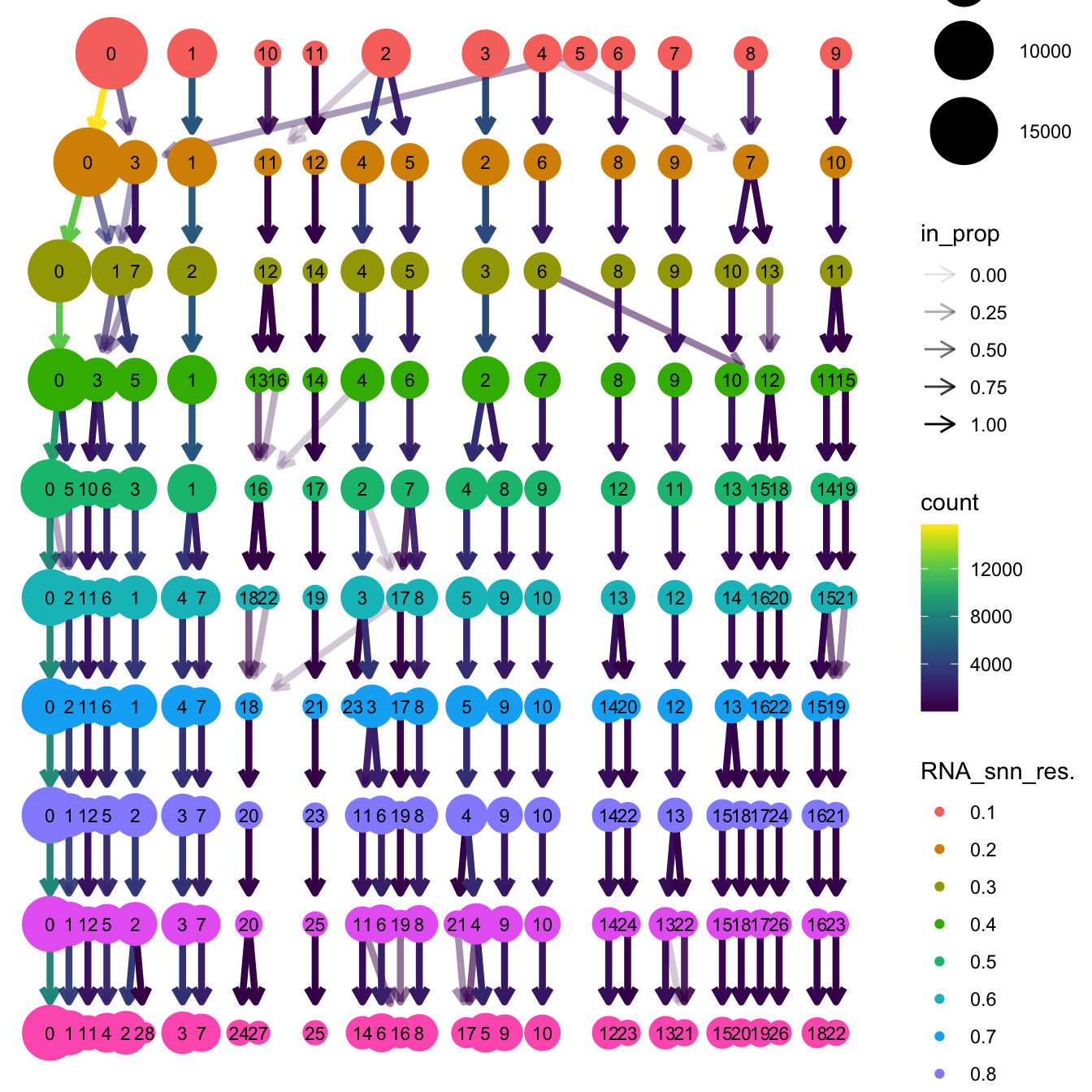

Past versions of clustree-1.png

Version	Author	Date
781f596	Gunjan Dixit	2024-10-01

Based on the clustering tree, we chose an intermediate/optimum resolution where the clustering results are the most stable, with the least amount of shuffling cells.

opt_res <- "RNA_snn_res.0.4"  
n <- nlevels(seu_obj$RNA_snn_res.0.4)
seu_obj$RNA_snn_res.0.4 <- factor(seu_obj$RNA_snn_res.0.4, levels = seq(0,n-1))
seu_obj$seurat_clusters <- NULL
seu_obj$cluster <- seu_obj$RNA_snn_res.0.4
Idents(seu_obj) <- seu_obj$cluster

UMAP after clustering

Defining colours for each cell-type to be consistent with other age-related/cell type composition plots.

my_colors <- c(
  "B cells" = "steelblue",
  "CD4 T cells" = "brown",
  "Double negative T cells" = "gold",
  "CD8 T cells" = "lightgreen",
  "Pre B/T cells" = "orchid",
  "Innate lymphoid cells" = "tan",
  "Natural Killer cells" = "blueviolet",
  "Macrophages" = "green4",
  "Cycling T cells" = "turquoise",
  "Dendritic cells" = "grey80",
  "Gamma delta T cells" = "mediumvioletred",
  "Epithelial lineage" = "darkorange",
  "Granulocytes" = "olivedrab",
  "Fibroblast lineage" = "lavender",
  "None" = "white",
  "Monocytes" = "peachpuff",
  "Endothelial lineage" = "cadetblue",
  "SMG duct" = "lightpink",
  "Neuroendocrine" = "skyblue",
  "Doublet query/Other" = "#d62728"
)

UMAP displaying clusters at opt_res resolution and Broad cell Labels Level 3.

p1 <- DimPlot(seu_obj, reduction = "umap", raster = FALSE ,repel = TRUE, label = TRUE,label.size = 3.5, group.by = opt_res) +  NoLegend()

p2 <- DimPlot(seu_obj, reduction = "umap", raster = FALSE, repel = TRUE, label = TRUE, label.size = 3.5, group.by = "Broad_cell_label_3") + 
  scale_colour_manual(values = my_colors) + 
  ggtitle(paste0(tissue, ": UMAP (Azimuth Labels)")) 


p1 / p2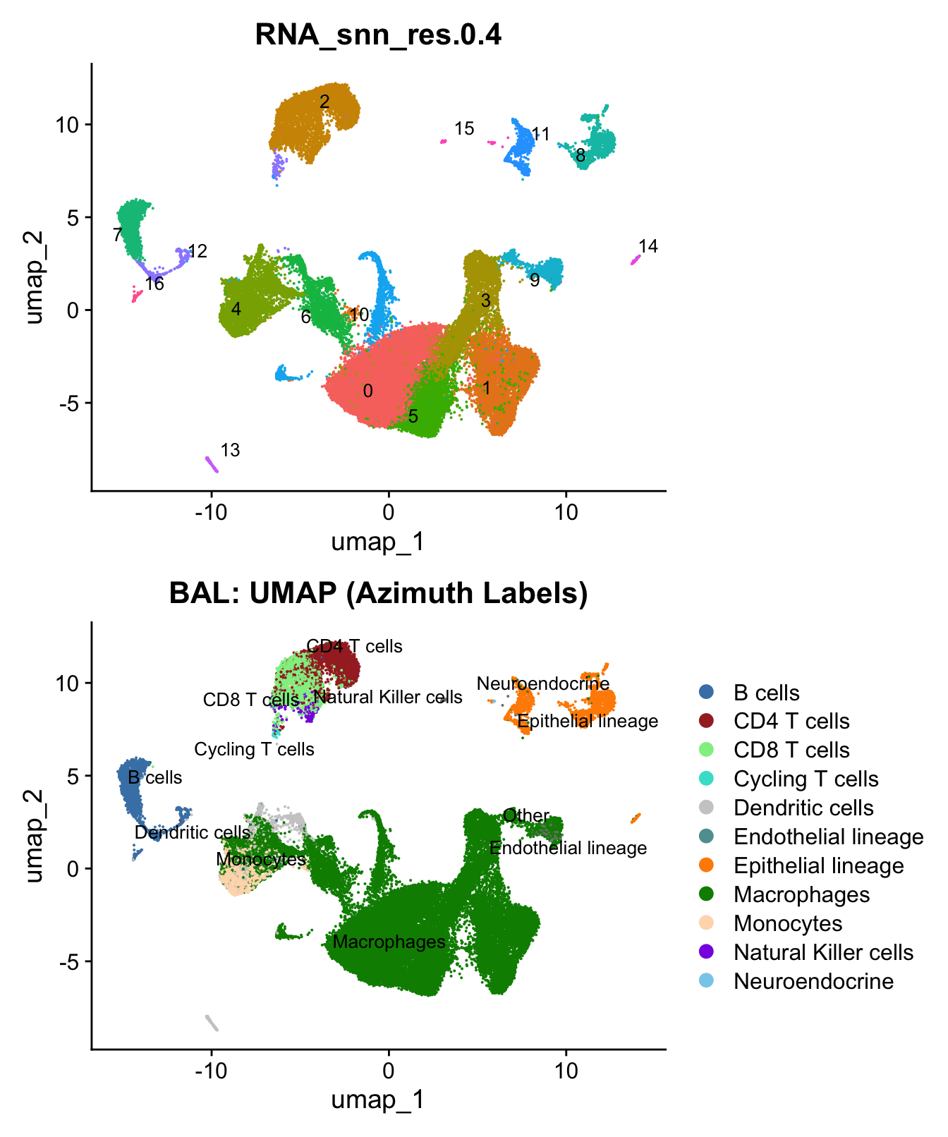 

Past versions of umap_after_clustering-1.png

Version	Author	Date
781f596	Gunjan Dixit	2024-10-01

Marker Gene Analysis

Here is the link to marker gene analysis of BAL (without ambient removal) BAL_withoutDecontX_res.0.4

seu_obj <- JoinLayers(seu_obj)
paed.markers <- FindAllMarkers(seu_obj, only.pos = TRUE, min.pct = 0.25, logfc.threshold = 0.25)

Extracting top 5 genes per cluster for visualization. The ‘top5’ contains the top 5 genes with the highest weighted average avg_log2FC within each cluster and the ‘best.wilcox.gene.per.cluster’ contains the single best gene with the highest weighted average avg_log2FC for each cluster.

paed.markers %>%
    group_by(cluster) %>% unique() %>% 
    top_n(n = 5, wt = avg_log2FC) -> top5

paed.markers %>%
    group_by(cluster) %>% 
    slice_head(n=1) %>% 
    pull(gene) -> best.wilcox.gene.per.cluster

best.wilcox.gene.per.cluster

 [1] "THBS1"   "DEFB1"   "IL32"    "NR1H3"   "SOCS3"   "TMEM74B" "VCAN"   
 [8] "CD79A"   "CTXN1"   "SLC11A1" "TK1"     "SLPI"    "ATP2A3"  "PTPRS"  
[15] "KRT13"   "KIT"     "JCHAIN" 

Marker gene expression in clusters

This heatmap depicts the expression of top five genes in each cluster.

DoHeatmap(seu_obj, features = top5$gene) + NoLegend()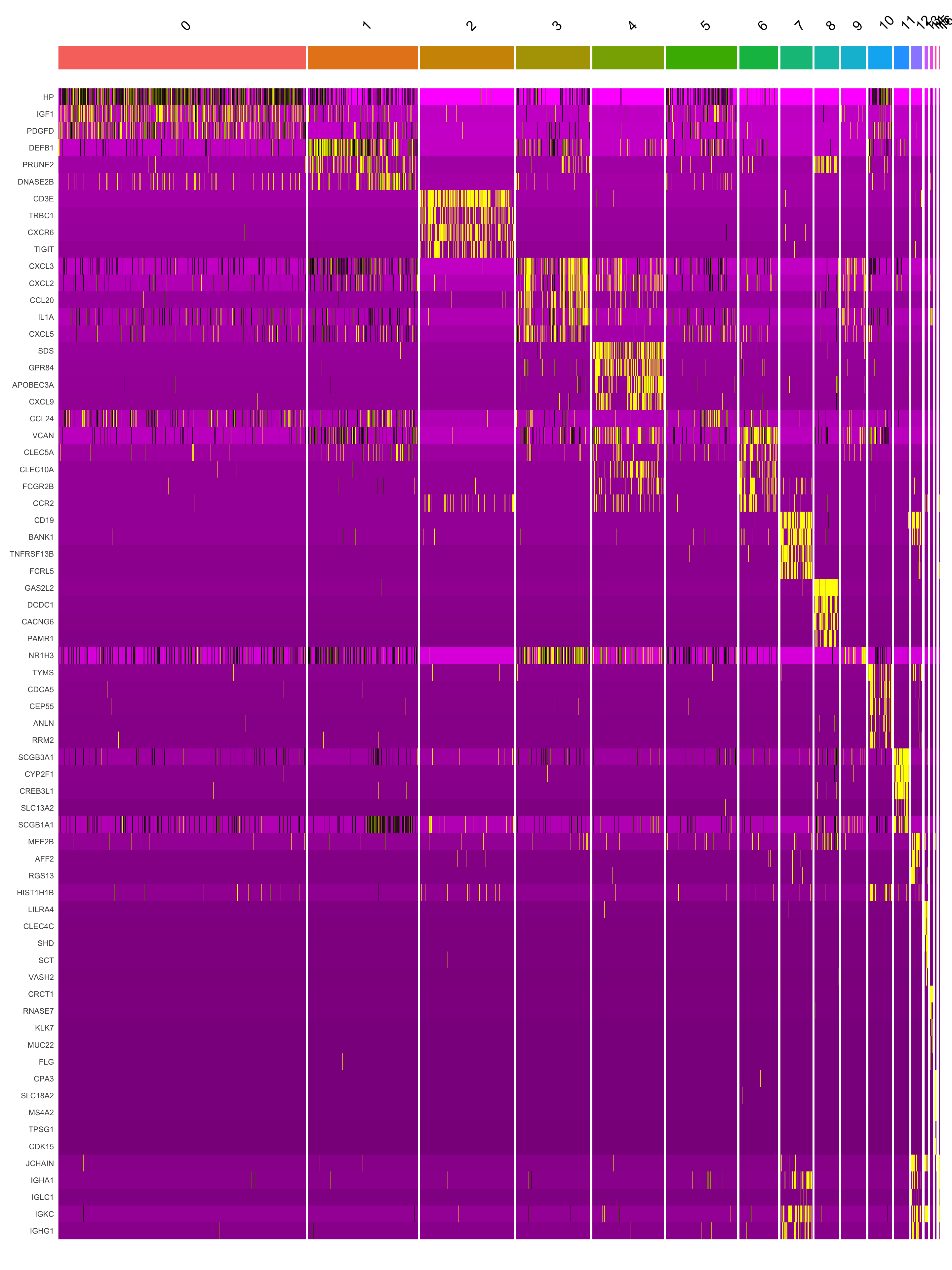

Past versions of top5_markers_heatmap-1.png

Version	Author	Date
781f596	Gunjan Dixit	2024-10-01

Violin plot shows the expression of top marker gene per cluster.

VlnPlot(seu_obj, features=best.wilcox.gene.per.cluster, ncol = 2, raster = FALSE, pt.size = FALSE)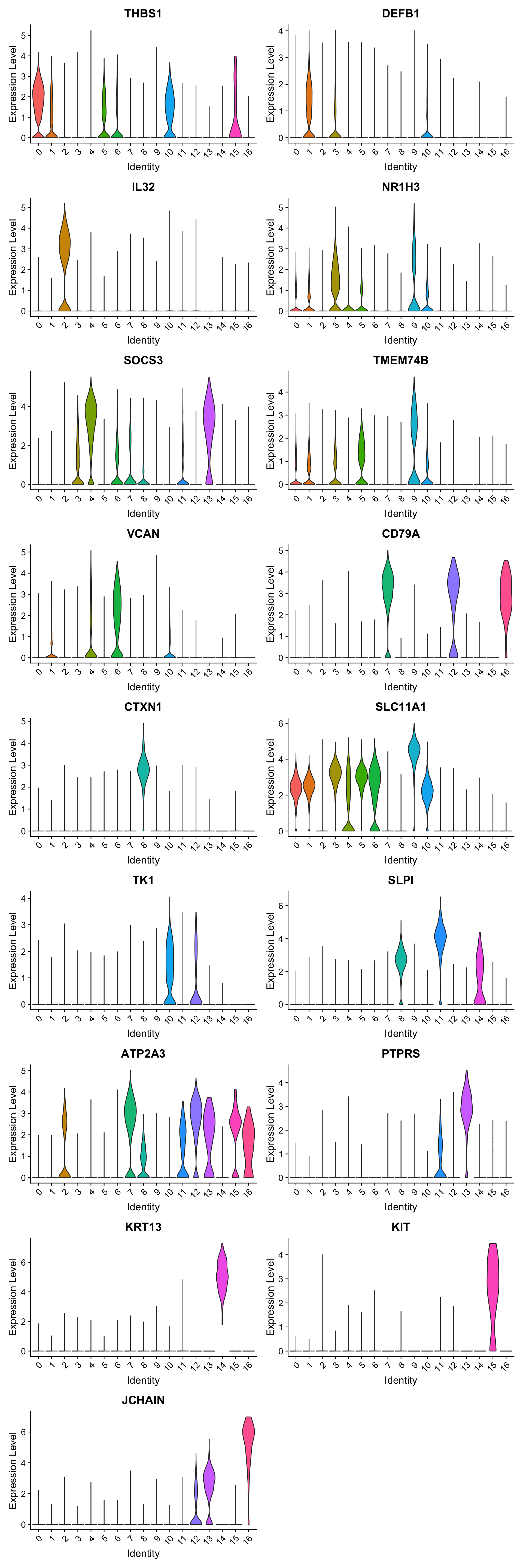

Past versions of top_marker_violinplot-1.png

Version	Author	Date
781f596	Gunjan Dixit	2024-10-01

Feature plot shows the expression of top marker genes per cluster.

FeaturePlot(seu_obj,features=best.wilcox.gene.per.cluster, reduction = 'umap', raster = FALSE, ncol = 2)

Past versions of top_marker_featureplot-1.png

Version	Author	Date
781f596	Gunjan Dixit	2024-10-01

Top 10 marker genes from Seurat

## Seurat top markers
top10 <- paed.markers %>%
    group_by(cluster) %>%
    top_n(n = 10, wt = avg_log2FC) %>%
    ungroup() %>%
    distinct(gene, .keep_all = TRUE) %>%
    arrange(cluster, desc(avg_log2FC))

cluster_colors <- paletteer::paletteer_d("pals::glasbey")[factor(top10$cluster)]

DotPlot(seu_obj,    
        features = unique(top10$gene),
        group.by = opt_res,
        cols = c("azure1", "blueviolet"),
        dot.scale = 3, assay = "RNA") +
    RotatedAxis() +
    FontSize(y.text = 8, x.text = 12) +
    labs(y = element_blank(), x = element_blank()) +
    coord_flip() +
    theme(axis.text.y = element_text(color = cluster_colors)) +
    ggtitle("Top 10 marker genes per cluster (Seurat)")

Warning: Vectorized input to `element_text()` is not officially supported.
ℹ Results may be unexpected or may change in future versions of ggplot2.

Past versions of unnamed-chunk-1-1.png

Version	Author	Date
781f596	Gunjan Dixit	2024-10-01

Extract markers for each cluster

This section extracts marker genes for each cluster and save them as a CSV file.

out_markers <- here("output",
            "CSV", 
            paste(tissue,"_Marker_gene_clusters_withoutDecontX.",opt_res, sep = ""))

dir.create(out_markers, recursive = TRUE, showWarnings = FALSE)

for (cl in unique(paed.markers$cluster)) {
  cluster_data <- paed.markers %>% dplyr::filter(cluster == cl)
  file_name <- here(out_markers, paste0("G000231_Neeland_",tissue, "_cluster_", cl, ".csv"))
  write.csv(cluster_data, file = file_name)
}

Update Macro labels

  cell_labels <- readxl::read_excel(here("data/Cell_labels_Mel_v2/earlyAIR_BAL_withoutDecontX_annotations_03.10.24_with broad label and flow label.xlsx"))
new_cluster_names <- cell_labels %>% 
  dplyr::select(cluster, annotation) %>% 
  deframe()

seu_obj <- RenameIdents(seu_obj, new_cluster_names)
seu_obj@meta.data$cell_labels <- Idents(seu_obj)

p3 <- DimPlot(seu_obj, reduction = "umap", raster = FALSE, repel = TRUE, label = TRUE, label.size = 3.5) + ggtitle(paste0(tissue, ": UMAP with Updated cell types"))

p3

Past versions of unnamed-chunk-2-1.png

Version	Author	Date
0f07f72	Gunjan Dixit	2024-10-07

Reclustering Macro polulation

Here is the link to marker gene analysis of Macrophages in BAL (without ambient removal) BAL_macro_withoutDecontX_res.0.7

Clusters corresponding to macrophage cell type are-

idx <- which(Idents(seu_obj) %in% c("macrophages"))
paed_sub <- seu_obj[,idx]
paed_sub@meta.data$donor <- sub("_\\d+$", "", paed_sub@meta.data$donor_id)
paed_sub

An object of class Seurat 
17529 features across 32502 samples within 1 assay 
Active assay: RNA (17529 features, 2000 variable features)
 3 layers present: counts, data, scale.data
 2 dimensional reductions calculated: pca, umap

paed_sub <- paed_sub %>%
  NormalizeData() %>%
  FindVariableFeatures() %>%
  ScaleData() %>%
  RunPCA() 
  
paed_sub <- RunUMAP(paed_sub, dims = 1:30, reduction = "pca", reduction.name = "umap.new")

meta_data_columns <- colnames(paed_sub@meta.data)
columns_to_remove <- grep("^RNA_snn_res", meta_data_columns, value = TRUE)
paed_sub@meta.data <- paed_sub@meta.data[, !(colnames(paed_sub@meta.data) %in% columns_to_remove)]


resolutions <- seq(0.1, 1, by = 0.1)
paed_sub <- FindNeighbors(paed_sub, reduction = "pca", dims = 1:30)
paed_sub <- FindClusters(paed_sub, resolution = resolutions, algorithm = 3)

Modularity Optimizer version 1.3.0 by Ludo Waltman and Nees Jan van Eck

Number of nodes: 32502
Number of edges: 1049780

Running smart local moving algorithm...
Maximum modularity in 10 random starts: 0.9687
Number of communities: 8
Elapsed time: 25 seconds
Modularity Optimizer version 1.3.0 by Ludo Waltman and Nees Jan van Eck

Number of nodes: 32502
Number of edges: 1049780

Running smart local moving algorithm...
Maximum modularity in 10 random starts: 0.9539
Number of communities: 10
Elapsed time: 26 seconds
Modularity Optimizer version 1.3.0 by Ludo Waltman and Nees Jan van Eck

Number of nodes: 32502
Number of edges: 1049780

Running smart local moving algorithm...
Maximum modularity in 10 random starts: 0.9398
Number of communities: 11
Elapsed time: 25 seconds
Modularity Optimizer version 1.3.0 by Ludo Waltman and Nees Jan van Eck

Number of nodes: 32502
Number of edges: 1049780

Running smart local moving algorithm...
Maximum modularity in 10 random starts: 0.9263
Number of communities: 12
Elapsed time: 24 seconds
Modularity Optimizer version 1.3.0 by Ludo Waltman and Nees Jan van Eck

Number of nodes: 32502
Number of edges: 1049780

Running smart local moving algorithm...
Maximum modularity in 10 random starts: 0.9162
Number of communities: 16
Elapsed time: 21 seconds
Modularity Optimizer version 1.3.0 by Ludo Waltman and Nees Jan van Eck

Number of nodes: 32502
Number of edges: 1049780

Running smart local moving algorithm...
Maximum modularity in 10 random starts: 0.9082
Number of communities: 18
Elapsed time: 21 seconds
Modularity Optimizer version 1.3.0 by Ludo Waltman and Nees Jan van Eck

Number of nodes: 32502
Number of edges: 1049780

Running smart local moving algorithm...
Maximum modularity in 10 random starts: 0.9012
Number of communities: 21
Elapsed time: 20 seconds
Modularity Optimizer version 1.3.0 by Ludo Waltman and Nees Jan van Eck

Number of nodes: 32502
Number of edges: 1049780

Running smart local moving algorithm...
Maximum modularity in 10 random starts: 0.8944
Number of communities: 21
Elapsed time: 20 seconds
Modularity Optimizer version 1.3.0 by Ludo Waltman and Nees Jan van Eck

Number of nodes: 32502
Number of edges: 1049780

Running smart local moving algorithm...
Maximum modularity in 10 random starts: 0.8877
Number of communities: 23
Elapsed time: 20 seconds
Modularity Optimizer version 1.3.0 by Ludo Waltman and Nees Jan van Eck

Number of nodes: 32502
Number of edges: 1049780

Running smart local moving algorithm...
Maximum modularity in 10 random starts: 0.8815
Number of communities: 24
Elapsed time: 19 seconds

DimHeatmap(paed_sub, dims = 1:10, cells = 500, balanced = TRUE)

Past versions of unnamed-chunk-4-1.png

Version	Author	Date
0f07f72	Gunjan Dixit	2024-10-07

clustree(paed_sub, prefix = "RNA_snn_res.")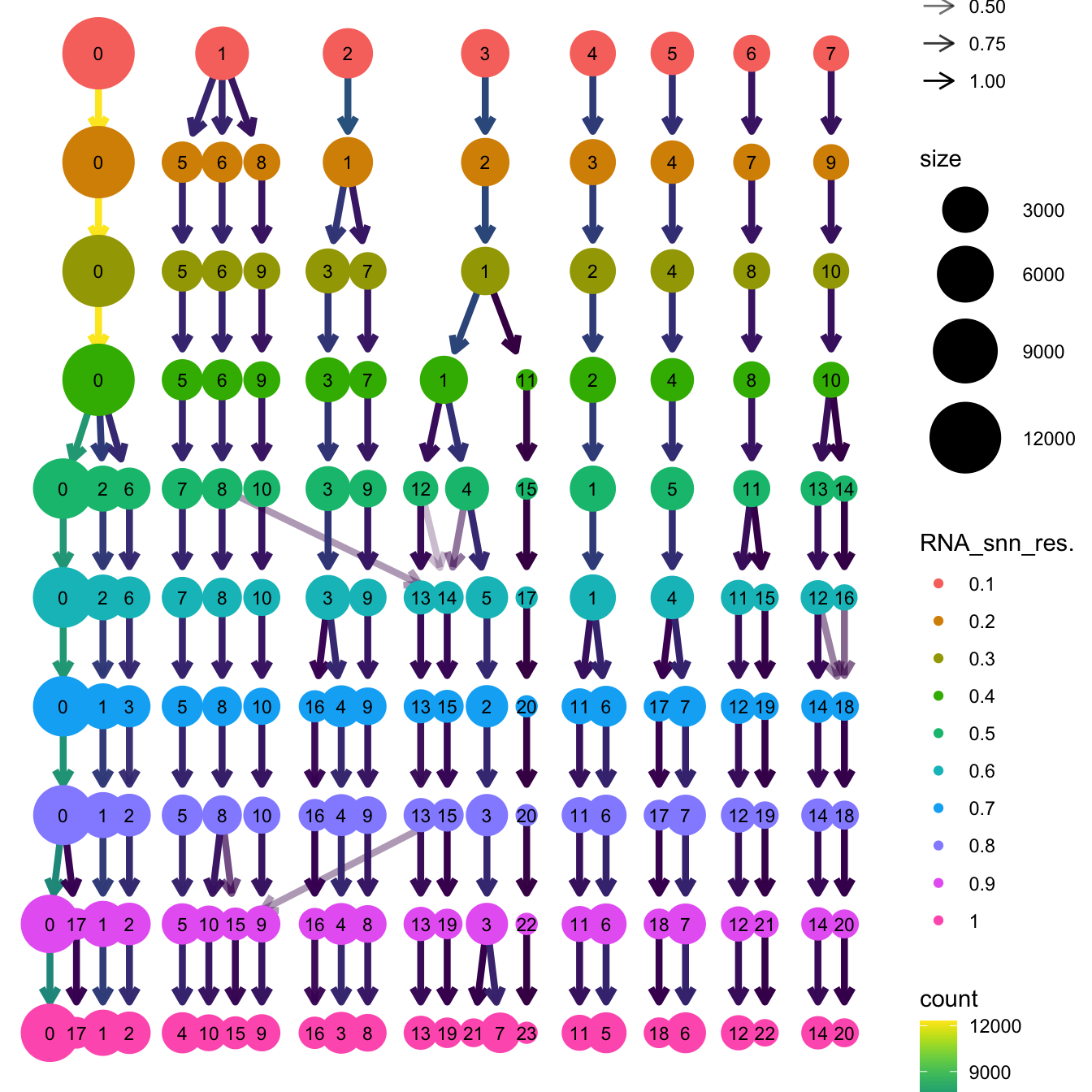

Past versions of unnamed-chunk-4-2.png

Version	Author	Date
0f07f72	Gunjan Dixit	2024-10-07

opt_res <- "RNA_snn_res.0.7"  
n <- nlevels(paed_sub$RNA_snn_res.0.7)
paed_sub$RNA_snn_res.0.7 <- factor(paed_sub$RNA_snn_res.0.7, levels = seq(0,n-1))
paed_sub$seurat_clusters <- NULL
Idents(paed_sub) <- paed_sub$RNA_snn_res.0.7

DimPlot(paed_sub, reduction = "umap.new", group.by = "RNA_snn_res.0.7", label = TRUE, label.size = 4.5, repel = TRUE, raster = FALSE )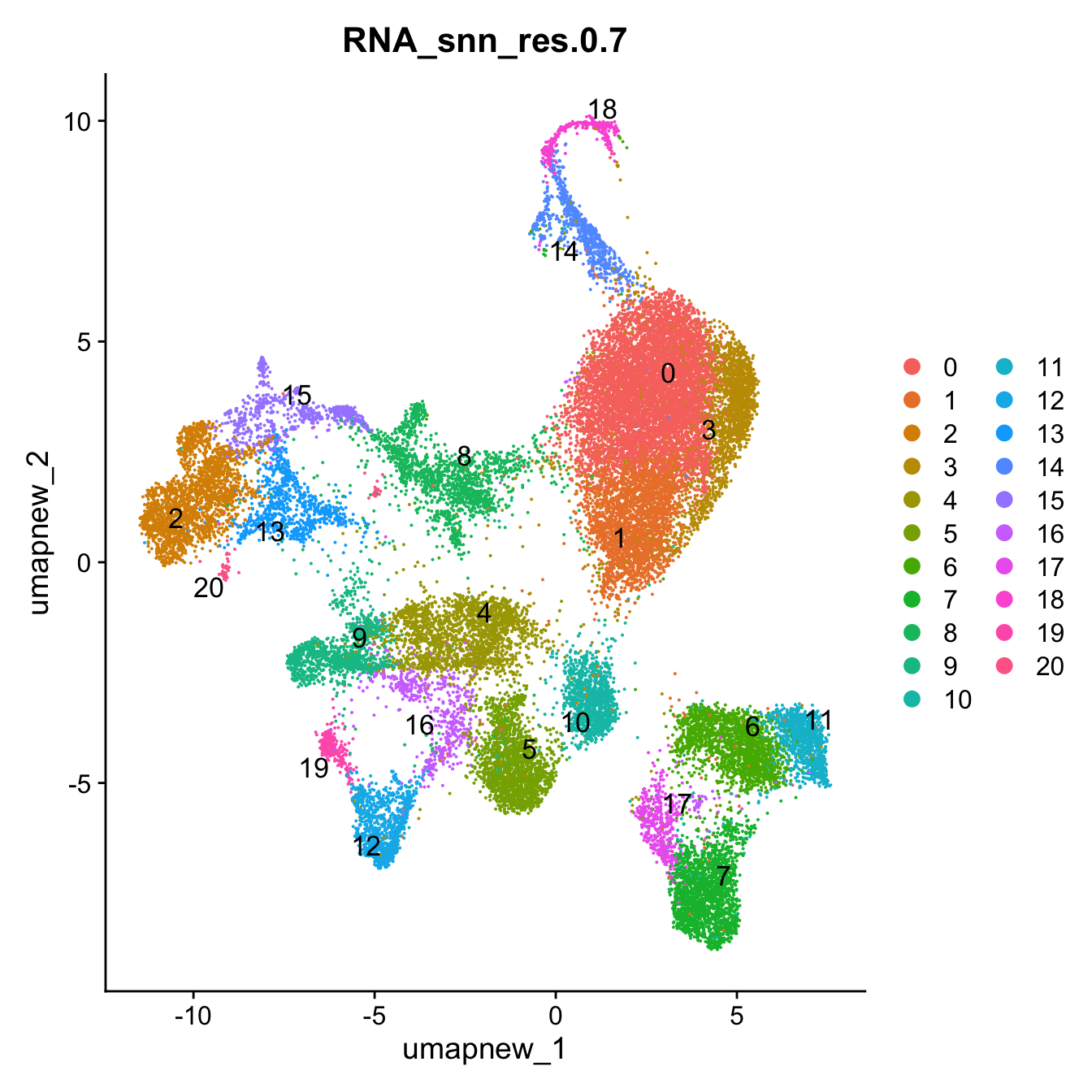

Past versions of unnamed-chunk-6-1.png

Version	Author	Date
0f07f72	Gunjan Dixit	2024-10-07

DimPlot(paed_sub, reduction = "umap.new", group.by = "predicted.ann_level_4", label = TRUE, label.size = 4.5, repel = TRUE, raster = FALSE )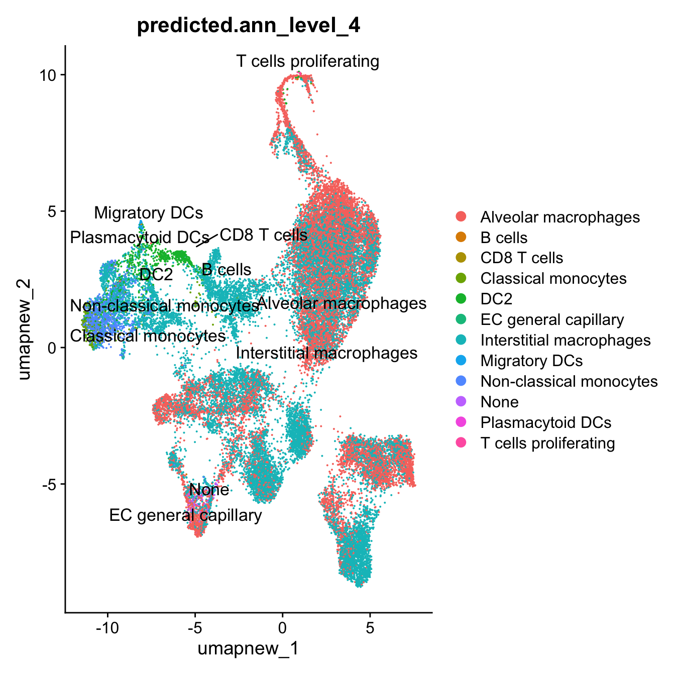

Azimuth Labels

## Finest level
DimPlot(paed_sub, reduction = "umap.new", group.by = "predicted.ann_finest_level", raster = FALSE, repel = TRUE, label = TRUE, label.size = 3.5)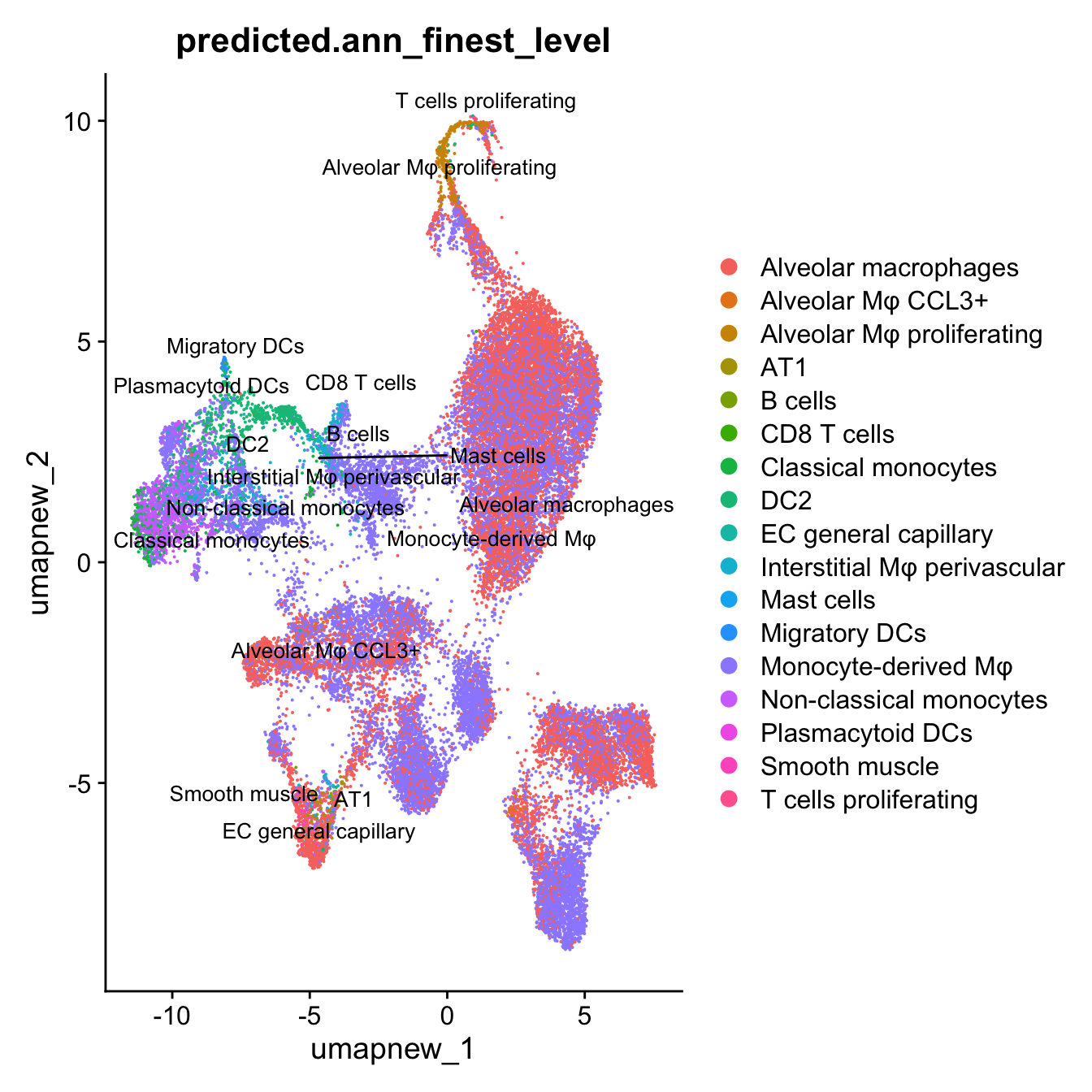 

Past versions of unnamed-chunk-8-1.png

Version	Author	Date
0f07f72	Gunjan Dixit	2024-10-07
781f596	Gunjan Dixit	2024-10-01

df_table <- as.data.frame(table(paed_sub$RNA_snn_res.0.7, paed_sub$predicted.ann_finest_level))
ggplot(df_table, aes(Var1, Freq, fill = Var2)) +
  geom_bar(stat = "identity") +
  labs(x = "RNA_snn_res.0.7", y = "Count", fill = "predicted ann_finest_level") +
  theme_minimal() +
  ggtitle("Stacked Bar Plot Azimuth predicted.ann_finest_level")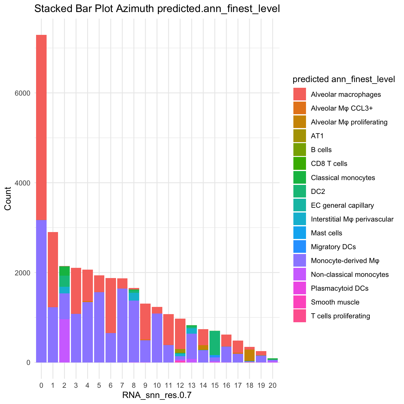

Past versions of unnamed-chunk-8-2.png

Version	Author	Date
781f596	Gunjan Dixit	2024-10-01

## Predicted_Level 5
DimPlot(paed_sub, reduction = "umap.new", group.by = "predicted.ann_level_4", raster = FALSE, repel = TRUE, label = TRUE, label.size = 3.5)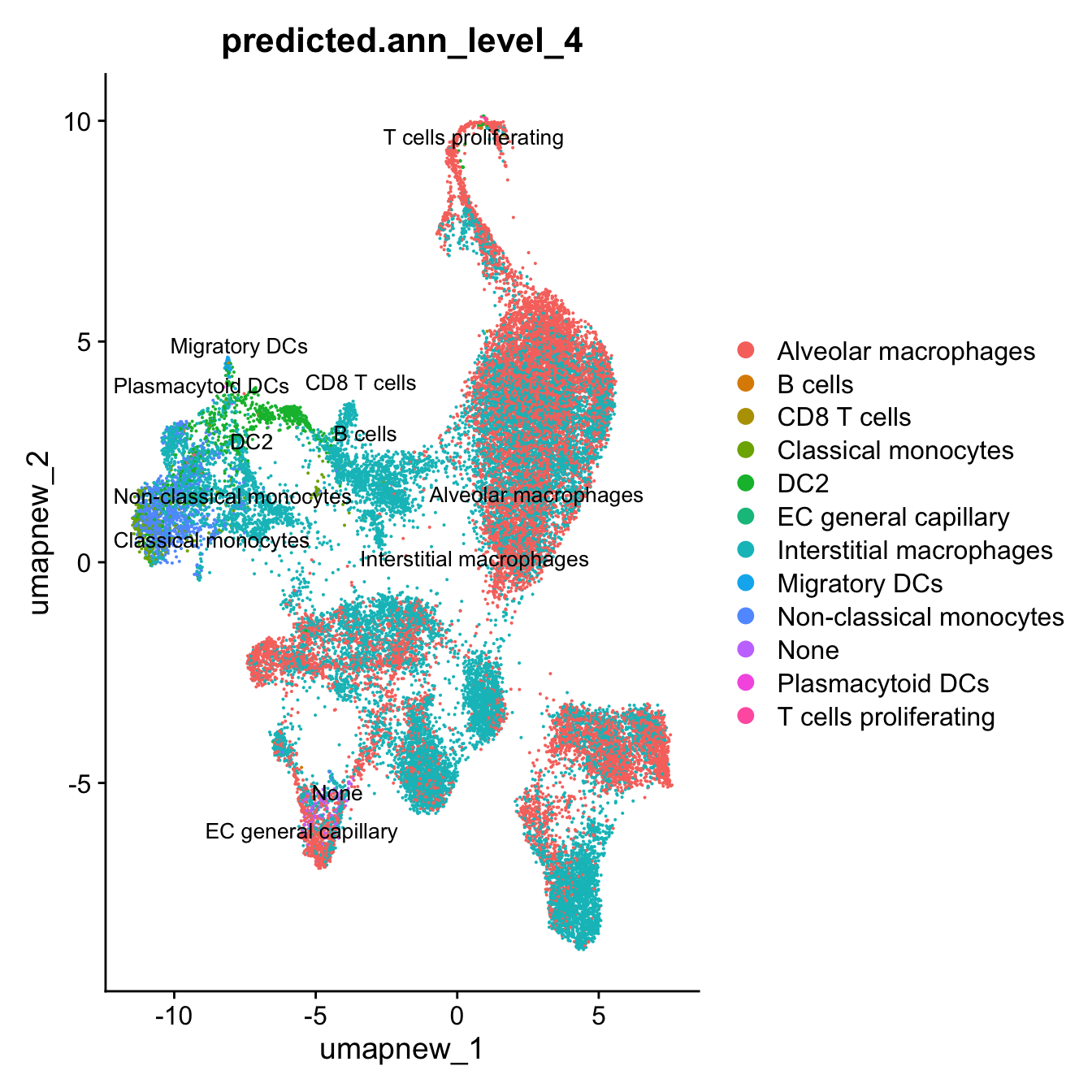 

df_table <- as.data.frame(table(paed_sub$RNA_snn_res.0.7, paed_sub$predicted.ann_level_4))

ggplot(df_table, aes(Var1, Freq, fill = Var2)) +
  geom_bar(stat = "identity") +
  labs(x = "RNA_snn_res.0.7", y = "Count", fill = "predicted ann_level_4") +
  theme_minimal() +
  ggtitle("Stacked Bar Plot Azimuth label")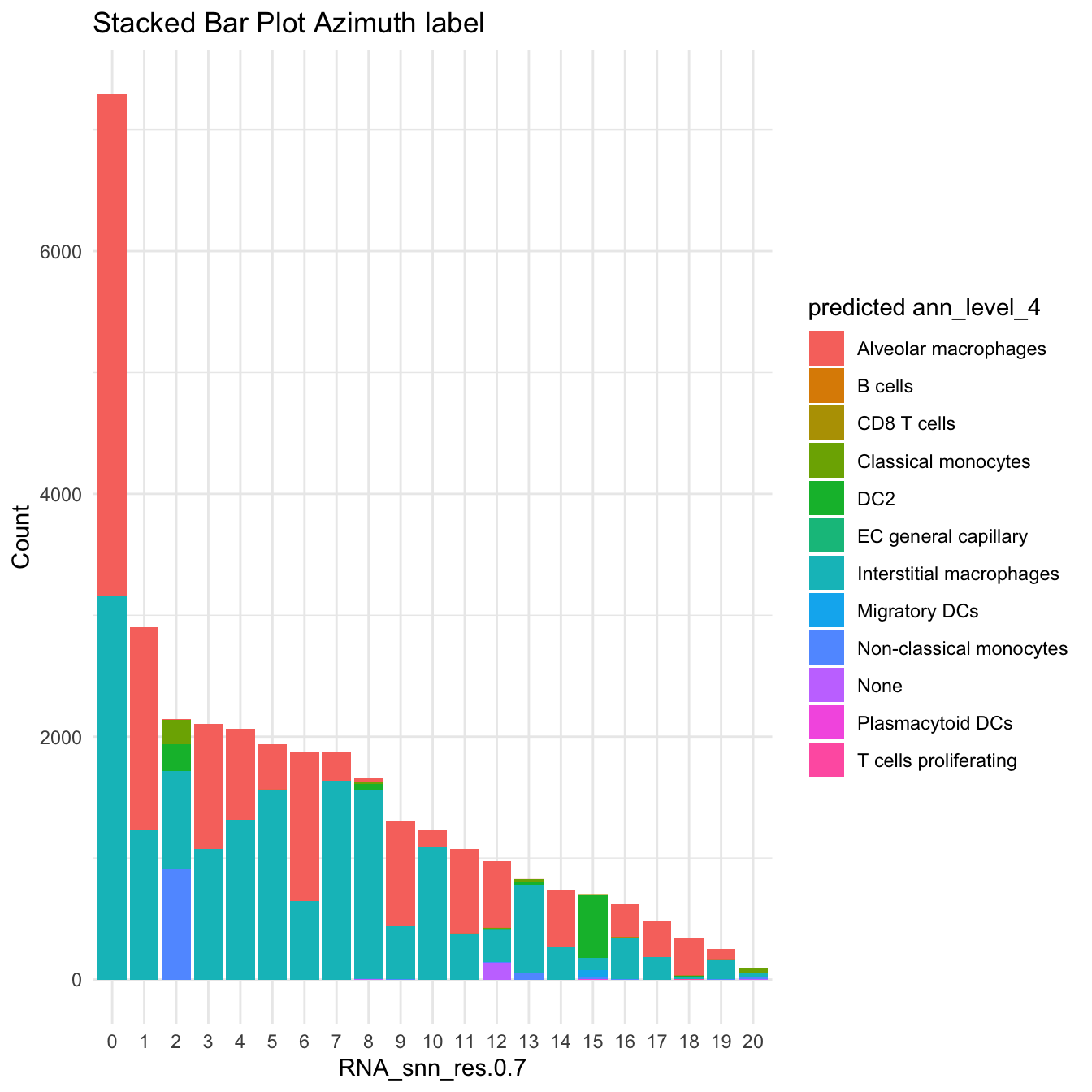

palette1 <- paletteer::paletteer_d("ggthemes::Classic_20")
palette2 <- paletteer::paletteer_d("Polychrome::light")
combined_palette <- unique(c(palette1, palette2))



p2 <- paed_sub@meta.data %>%
  dplyr::select(!!sym(opt_res), donor) %>%
  group_by(!!sym(opt_res), donor) %>%
  summarise(num = n()) %>%
  mutate(prop = num / sum(num)) %>%
  ggplot(aes(x = !!sym(opt_res), y = prop * 100, 
             fill = donor)) + 
  geom_bar(stat = "identity") +
  theme(axis.text.x = element_text(angle = 90, 
                                   vjust = 0.5, 
                                   hjust = 1,
                                   size = 8)) +
  labs(y = "% Cells", fill = "donor") +
  scale_fill_manual(values = combined_palette)

`summarise()` has grouped output by 'RNA_snn_res.0.7'. You can override using
the `.groups` argument.

# Combine the plots
p2 & theme( legend.text = element_text(size = 8),
                            legend.key.size = unit(3, "mm"))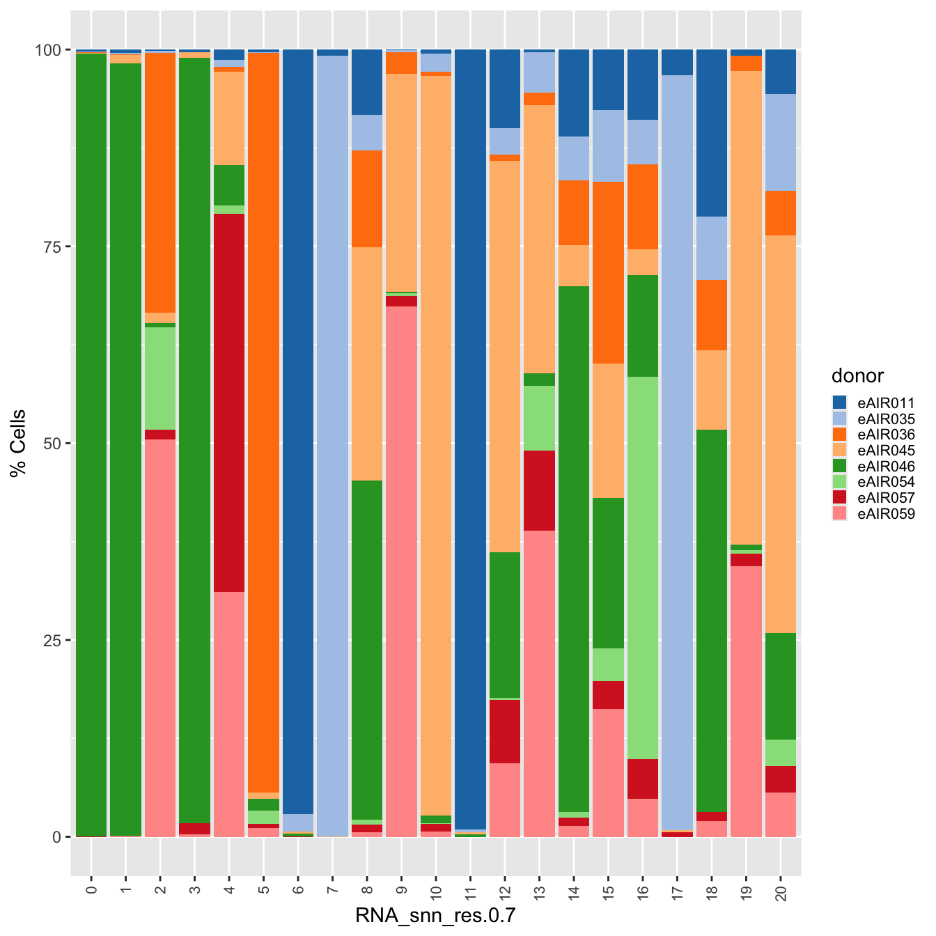

Past versions of unnamed-chunk-9-1.png

Version	Author	Date
0f07f72	Gunjan Dixit	2024-10-07

paed_sub.markers <- FindAllMarkers(paed_sub, only.pos = TRUE, min.pct = 0.25, logfc.threshold = 0.25)

Calculating cluster 0

Calculating cluster 1

Calculating cluster 2

Calculating cluster 3

Calculating cluster 4

Calculating cluster 5

Calculating cluster 6

Calculating cluster 7

Calculating cluster 8

Calculating cluster 9

Calculating cluster 10

Calculating cluster 11

Calculating cluster 12

Calculating cluster 13

Calculating cluster 14

Calculating cluster 15

Calculating cluster 16

Calculating cluster 17

Calculating cluster 18

Calculating cluster 19

Calculating cluster 20

paed_sub.markers %>%
    group_by(cluster) %>% unique() %>% 
    top_n(n = 10, wt = avg_log2FC) -> top10

paed_sub.markers %>%
    group_by(cluster) %>% 
    slice_head(n=1) %>% 
    pull(gene) -> best.wilcox.gene.per.cluster

best.wilcox.gene.per.cluster

 [1] "THBS1"    "APP"      "SERPINB9" "SENP3"    "ABCA1"    "PRDX2"   
 [7] "DEFB1"    "ENPP4"    "VCAN"     "CXCL2"    "PLA1A"    "MT-ND3"  
[13] "RSRP1"    "SDS"      "E2F1"     "SERPINB9" "SQSTM1"   "NRP2"    
[19] "MKI67"    "CCL20"    "PROK2"   

Feature plot shows the expression of top marker genes per cluster.

FeaturePlot(paed_sub,features=best.wilcox.gene.per.cluster, reduction = 'umap.new', raster = FALSE, ncol = 2, label = TRUE)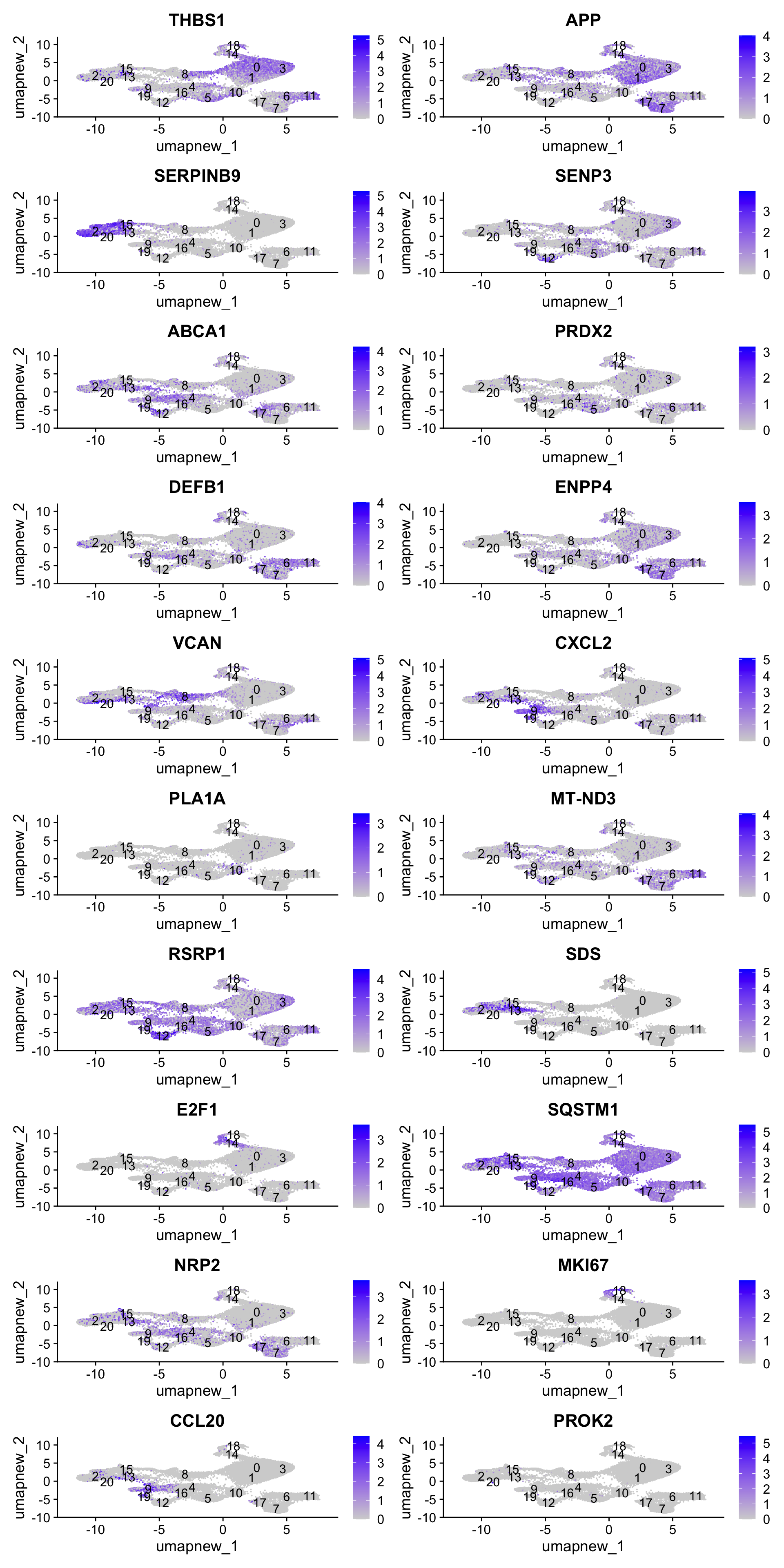

Top 10 marker genes from Seurat

## Seurat top markers
top10 <- paed_sub.markers %>%
    group_by(cluster) %>%
    top_n(n = 10, wt = avg_log2FC) %>%
    ungroup() %>%
    distinct(gene, .keep_all = TRUE) %>%
    arrange(cluster, desc(avg_log2FC))

cluster_colors <- paletteer::paletteer_d("pals::glasbey")[factor(top10$cluster)]

DotPlot(paed_sub,    
        features = unique(top10$gene),
        group.by = opt_res,
        cols = c("azure1", "blueviolet"),
        dot.scale = 3, assay = "RNA") +
    RotatedAxis() +
    FontSize(y.text = 8, x.text = 12) +
    labs(y = element_blank(), x = element_blank()) +
    coord_flip() +
    theme(axis.text.y = element_text(color = cluster_colors)) +
    ggtitle("Top 10 marker genes per cluster (Seurat)")

Warning: Vectorized input to `element_text()` is not officially supported.
ℹ Results may be unexpected or may change in future versions of ggplot2.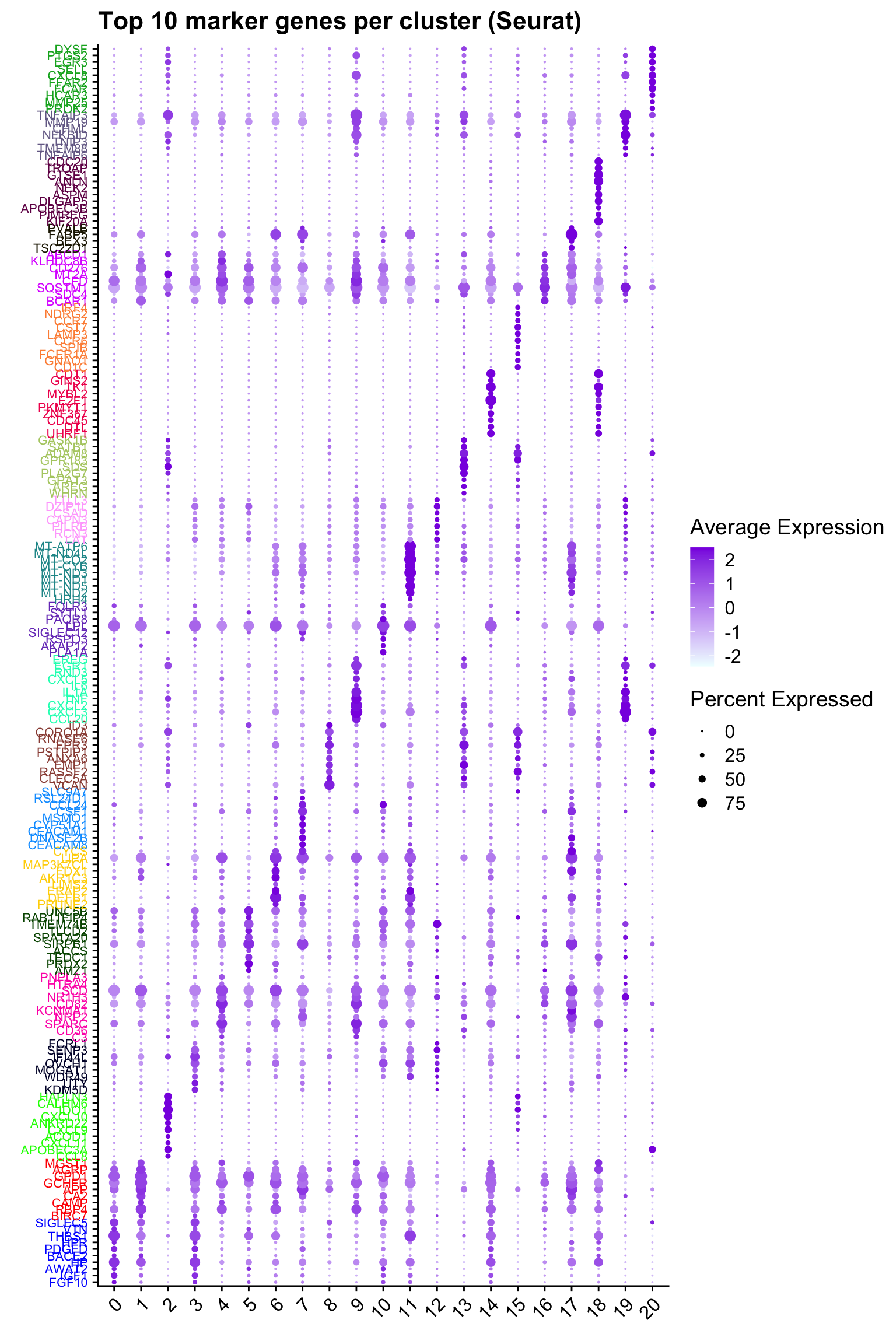

Past versions of unnamed-chunk-12-1.png

Version	Author	Date
0f07f72	Gunjan Dixit	2024-10-07

out_markers <- here("output",
            "CSV", 
            paste(tissue,"_Marker_genes_Reclustered_macro_population.withoutDecontX.",opt_res, sep = ""))

dir.create(out_markers, recursive = TRUE, showWarnings = FALSE)

for (cl in unique(paed_sub.markers$cluster)) {
  cluster_data <- paed_sub.markers %>% dplyr::filter(cluster == cl)
  file_name <- here(out_markers, paste0("G000231_Neeland_",tissue, "_cluster_", cl, ".csv"))
  write.csv(cluster_data, file = file_name)
}

Save subclustered SEU object

out2 <- here("output",
            "RDS", "AllBatches_Subclustering_SEUs", tissue,
             paste0("G000231_Neeland_",tissue,".macro_population.subclusters_without_DecontX.SEU.rds"))
#dir.create(out2)
if (!file.exists(out2)) {
  saveRDS(paed_sub, file = out2)
}

Reclustering T/NK polulation

Here is the link to marker gene analysis of Macrophages in BAL (without ambient removal) BAL_Tcell_withoutDecontX_res.0.4

idx <- which(Idents(seu_obj) %in% "T/NK cells")
paed_sub <- seu_obj[,idx]
paed_sub

An object of class Seurat 
17529 features across 4631 samples within 1 assay 
Active assay: RNA (17529 features, 2000 variable features)
 3 layers present: counts, data, scale.data
 2 dimensional reductions calculated: pca, umap

paed_sub <- paed_sub %>%
  NormalizeData() %>%
  FindVariableFeatures() %>%
  ScaleData() %>%
  RunPCA() 
  
paed_sub <- RunUMAP(paed_sub, dims = 1:30, reduction = "pca", reduction.name = "umap.new")

meta_data_columns <- colnames(paed_sub@meta.data)
columns_to_remove <- grep("^RNA_snn_res", meta_data_columns, value = TRUE)
paed_sub@meta.data <- paed_sub@meta.data[, !(colnames(paed_sub@meta.data) %in% columns_to_remove)]


resolutions <- seq(0.1, 1, by = 0.1)
paed_sub <- FindNeighbors(paed_sub, reduction = "pca", dims = 1:30)
paed_sub <- FindClusters(paed_sub, resolution = resolutions, algorithm = 3)

Modularity Optimizer version 1.3.0 by Ludo Waltman and Nees Jan van Eck

Number of nodes: 4631
Number of edges: 181992

Running smart local moving algorithm...
Maximum modularity in 10 random starts: 0.9321
Number of communities: 4
Elapsed time: 1 seconds
Modularity Optimizer version 1.3.0 by Ludo Waltman and Nees Jan van Eck

Number of nodes: 4631
Number of edges: 181992

Running smart local moving algorithm...
Maximum modularity in 10 random starts: 0.9048
Number of communities: 8
Elapsed time: 1 seconds
Modularity Optimizer version 1.3.0 by Ludo Waltman and Nees Jan van Eck

Number of nodes: 4631
Number of edges: 181992

Running smart local moving algorithm...
Maximum modularity in 10 random starts: 0.8828
Number of communities: 9
Elapsed time: 1 seconds
Modularity Optimizer version 1.3.0 by Ludo Waltman and Nees Jan van Eck

Number of nodes: 4631
Number of edges: 181992

Running smart local moving algorithm...
Maximum modularity in 10 random starts: 0.8660
Number of communities: 11
Elapsed time: 1 seconds
Modularity Optimizer version 1.3.0 by Ludo Waltman and Nees Jan van Eck

Number of nodes: 4631
Number of edges: 181992

Running smart local moving algorithm...
Maximum modularity in 10 random starts: 0.8502
Number of communities: 11
Elapsed time: 1 seconds
Modularity Optimizer version 1.3.0 by Ludo Waltman and Nees Jan van Eck

Number of nodes: 4631
Number of edges: 181992

Running smart local moving algorithm...
Maximum modularity in 10 random starts: 0.8359
Number of communities: 12
Elapsed time: 1 seconds
Modularity Optimizer version 1.3.0 by Ludo Waltman and Nees Jan van Eck

Number of nodes: 4631
Number of edges: 181992

Running smart local moving algorithm...
Maximum modularity in 10 random starts: 0.8239
Number of communities: 13
Elapsed time: 1 seconds
Modularity Optimizer version 1.3.0 by Ludo Waltman and Nees Jan van Eck

Number of nodes: 4631
Number of edges: 181992

Running smart local moving algorithm...
Maximum modularity in 10 random starts: 0.8136
Number of communities: 15
Elapsed time: 1 seconds
Modularity Optimizer version 1.3.0 by Ludo Waltman and Nees Jan van Eck

Number of nodes: 4631
Number of edges: 181992

Running smart local moving algorithm...
Maximum modularity in 10 random starts: 0.8045
Number of communities: 17
Elapsed time: 1 seconds
Modularity Optimizer version 1.3.0 by Ludo Waltman and Nees Jan van Eck

Number of nodes: 4631
Number of edges: 181992

Running smart local moving algorithm...
Maximum modularity in 10 random starts: 0.7955
Number of communities: 17
Elapsed time: 1 seconds

DimHeatmap(paed_sub, dims = 1:10, cells = 500, balanced = TRUE)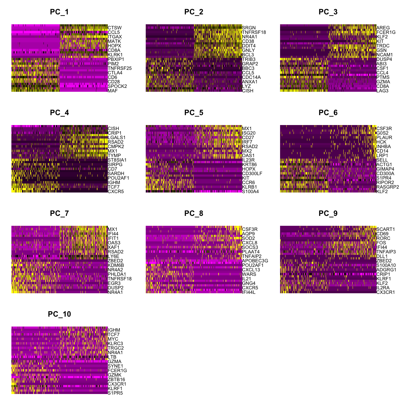

clustree(paed_sub, prefix = "RNA_snn_res.")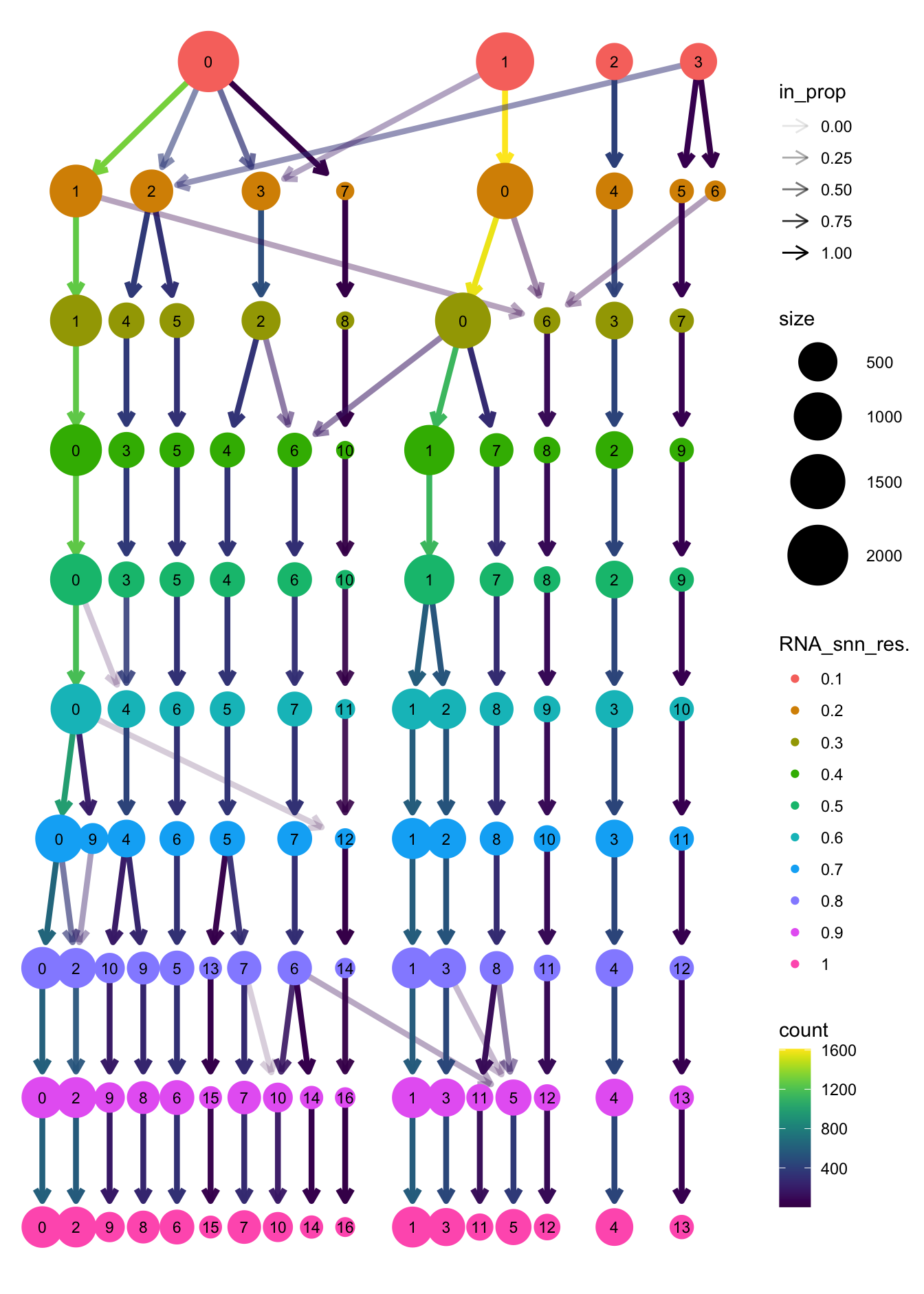

Past versions of unnamed-chunk-16-1.png

Version	Author	Date
0f07f72	Gunjan Dixit	2024-10-07

opt_res <- "RNA_snn_res.0.4"  
n <- nlevels(paed_sub$RNA_snn_res.0.4)
paed_sub$RNA_snn_res.0.4 <- factor(paed_sub$RNA_snn_res.0.4, levels = seq(0,n-1))
paed_sub$seurat_clusters <- NULL
paed_sub$cluster <- paed_sub$RNA_snn_res.0.4
Idents(paed_sub) <- paed_sub$cluster

paed_sub.markers <- FindAllMarkers(paed_sub, only.pos = TRUE, min.pct = 0.25, logfc.threshold = 0.25)

Calculating cluster 0

Calculating cluster 1

Calculating cluster 2

Calculating cluster 3

Calculating cluster 4

Calculating cluster 5

Calculating cluster 6

Calculating cluster 7

Calculating cluster 8

Calculating cluster 9

Calculating cluster 10

paed_sub.markers %>%
    group_by(cluster) %>% unique() %>% 
    top_n(n = 5, wt = avg_log2FC) -> top5

paed_sub.markers %>%
    group_by(cluster) %>% 
    slice_head(n=1) %>% 
    pull(gene) -> best.wilcox.gene.per.cluster

best.wilcox.gene.per.cluster

 [1] "CCL5"   "CD4"    "NMUR1"  "TCF7"   "GZMB"   "NCAM1"  "MAF"    "CXCR5" 
 [9] "CX3CR1" "KIT"    "TFEC"  

Feature plot shows the expression of top marker genes per cluster.

FeaturePlot(paed_sub,features=best.wilcox.gene.per.cluster, reduction = 'umap.new', raster = FALSE, ncol = 2, label = TRUE)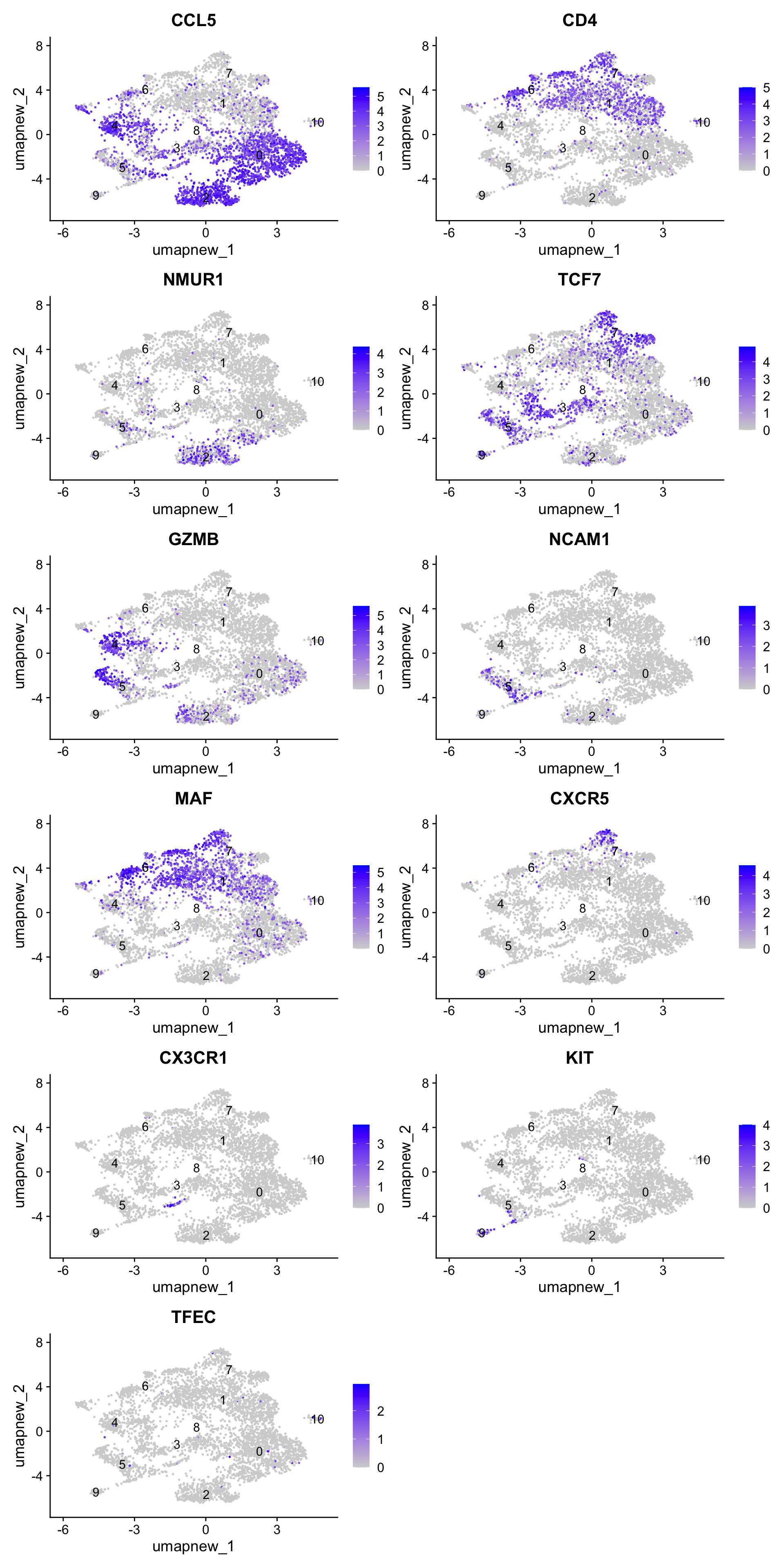

Top 10 marker genes from Seurat

## Seurat top markers
top10 <- paed_sub.markers %>%
    group_by(cluster) %>%
    top_n(n = 10, wt = avg_log2FC) %>%
    ungroup() %>%
    distinct(gene, .keep_all = TRUE) %>%
    arrange(cluster, desc(avg_log2FC))

cluster_colors <- paletteer::paletteer_d("pals::glasbey")[factor(top10$cluster)]

DotPlot(paed_sub,    
        features = unique(top10$gene),
        group.by = opt_res,
        cols = c("azure1", "blueviolet"),
        dot.scale = 3, assay = "RNA") +
    RotatedAxis() +
    FontSize(y.text = 8, x.text = 12) +
    labs(y = element_blank(), x = element_blank()) +
    coord_flip() +
    theme(axis.text.y = element_text(color = cluster_colors)) +
    ggtitle("Top 10 marker genes per cluster (Seurat)")

Warning: Vectorized input to `element_text()` is not officially supported.
ℹ Results may be unexpected or may change in future versions of ggplot2.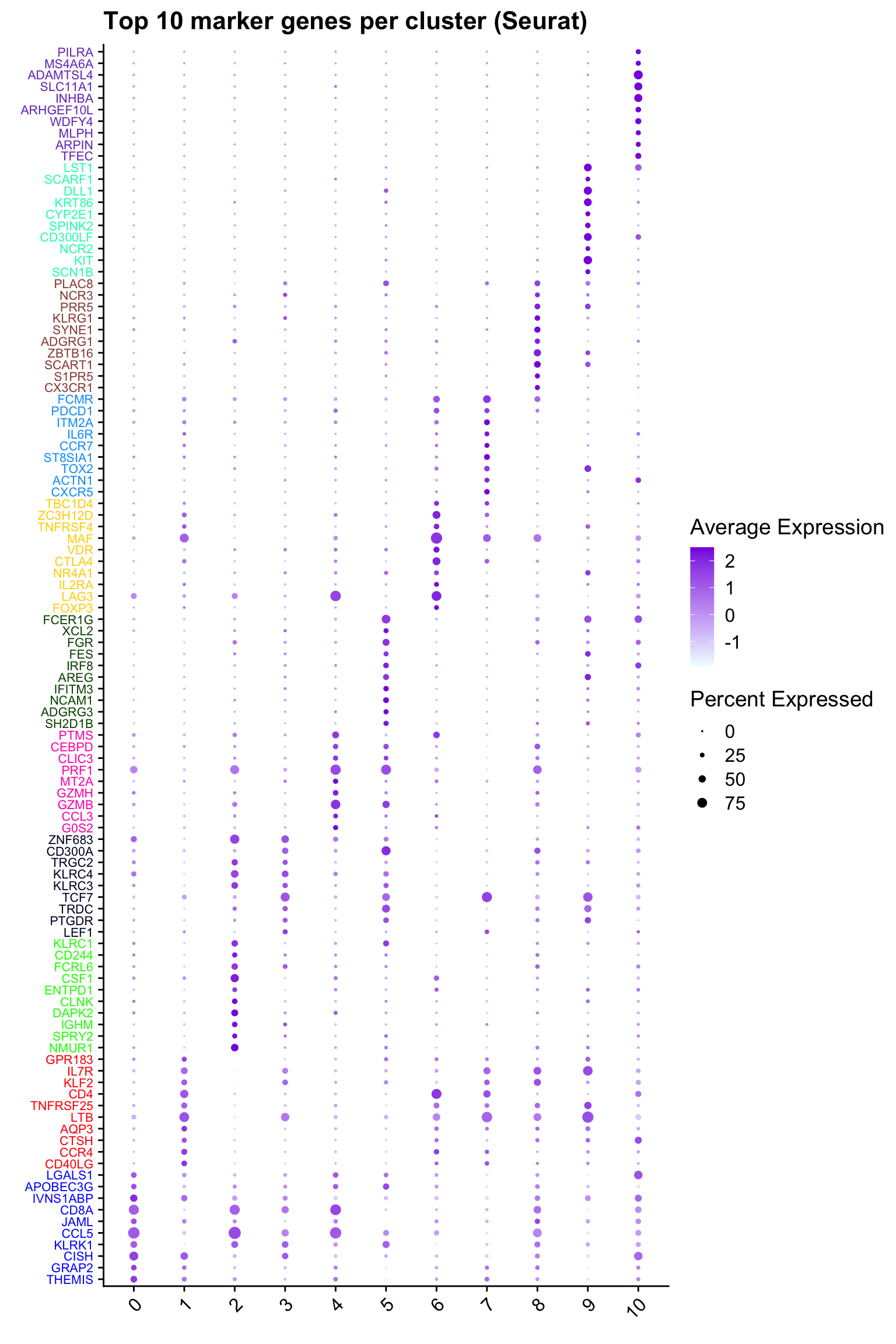

Past versions of unnamed-chunk-20-1.png

Version	Author	Date
0f07f72	Gunjan Dixit	2024-10-07

out_markers <- here("output",
            "CSV", 
            paste(tissue,"_Marker_genes_Reclustered_Tcell_population.withoutDecontX.",opt_res, sep = ""))

dir.create(out_markers, recursive = TRUE, showWarnings = FALSE)

for (cl in unique(paed_sub.markers$cluster)) {
  cluster_data <- paed_sub.markers %>% dplyr::filter(cluster == cl)
  file_name <- here(out_markers, paste0("G000231_Neeland_",tissue, "_cluster_", cl, ".csv"))
  write.csv(cluster_data, file = file_name)
}

Save subclustered SEU object

out2 <- here("output",
            "RDS", "AllBatches_Subclustering_SEUs", tissue,
             paste0("G000231_Neeland_",tissue,".Tcell_population.subclusters_without_DecontX.SEU.rds"))
#dir.create(out2)
if (!file.exists(out2)) {
  saveRDS(paed_sub, file = out2)
}

Reclustering Bcell polulation

Here is the link to marker gene analysis of Macrophages in BAL (without ambient removal) BAL_Bcell_withoutDecontX_res.0.4

idx <- which(Idents(seu_obj) %in% "B cells")
paed_sub <- seu_obj[,idx]
paed_sub

An object of class Seurat 
17529 features across 2176 samples within 1 assay 
Active assay: RNA (17529 features, 2000 variable features)
 3 layers present: counts, data, scale.data
 2 dimensional reductions calculated: pca, umap

paed_sub <- paed_sub %>%
  NormalizeData() %>%
  FindVariableFeatures() %>%
  ScaleData() %>%
  RunPCA() 
  
paed_sub <- RunUMAP(paed_sub, dims = 1:30, reduction = "pca", reduction.name = "umap.new")

meta_data_columns <- colnames(paed_sub@meta.data)
columns_to_remove <- grep("^RNA_snn_res", meta_data_columns, value = TRUE)
paed_sub@meta.data <- paed_sub@meta.data[, !(colnames(paed_sub@meta.data) %in% columns_to_remove)]


resolutions <- seq(0.1, 1, by = 0.1)
paed_sub <- FindNeighbors(paed_sub, reduction = "pca", dims = 1:30)
paed_sub <- FindClusters(paed_sub, resolution = resolutions, algorithm = 3)

Modularity Optimizer version 1.3.0 by Ludo Waltman and Nees Jan van Eck

Number of nodes: 2176
Number of edges: 85004

Running smart local moving algorithm...
Maximum modularity in 10 random starts: 0.9388
Number of communities: 4
Elapsed time: 0 seconds
Modularity Optimizer version 1.3.0 by Ludo Waltman and Nees Jan van Eck

Number of nodes: 2176
Number of edges: 85004

Running smart local moving algorithm...
Maximum modularity in 10 random starts: 0.9042
Number of communities: 6
Elapsed time: 0 seconds
Modularity Optimizer version 1.3.0 by Ludo Waltman and Nees Jan van Eck

Number of nodes: 2176
Number of edges: 85004

Running smart local moving algorithm...
Maximum modularity in 10 random starts: 0.8780
Number of communities: 7
Elapsed time: 0 seconds
Modularity Optimizer version 1.3.0 by Ludo Waltman and Nees Jan van Eck

Number of nodes: 2176
Number of edges: 85004

Running smart local moving algorithm...
Maximum modularity in 10 random starts: 0.8571
Number of communities: 7
Elapsed time: 0 seconds
Modularity Optimizer version 1.3.0 by Ludo Waltman and Nees Jan van Eck

Number of nodes: 2176
Number of edges: 85004

Running smart local moving algorithm...
Maximum modularity in 10 random starts: 0.8390
Number of communities: 7
Elapsed time: 0 seconds
Modularity Optimizer version 1.3.0 by Ludo Waltman and Nees Jan van Eck

Number of nodes: 2176
Number of edges: 85004

Running smart local moving algorithm...
Maximum modularity in 10 random starts: 0.8231
Number of communities: 9
Elapsed time: 0 seconds
Modularity Optimizer version 1.3.0 by Ludo Waltman and Nees Jan van Eck

Number of nodes: 2176
Number of edges: 85004

Running smart local moving algorithm...
Maximum modularity in 10 random starts: 0.8079
Number of communities: 9
Elapsed time: 0 seconds
Modularity Optimizer version 1.3.0 by Ludo Waltman and Nees Jan van Eck

Number of nodes: 2176
Number of edges: 85004

Running smart local moving algorithm...
Maximum modularity in 10 random starts: 0.7956
Number of communities: 11
Elapsed time: 0 seconds
Modularity Optimizer version 1.3.0 by Ludo Waltman and Nees Jan van Eck

Number of nodes: 2176
Number of edges: 85004

Running smart local moving algorithm...
Maximum modularity in 10 random starts: 0.7848
Number of communities: 12
Elapsed time: 0 seconds
Modularity Optimizer version 1.3.0 by Ludo Waltman and Nees Jan van Eck

Number of nodes: 2176
Number of edges: 85004

Running smart local moving algorithm...
Maximum modularity in 10 random starts: 0.7742
Number of communities: 12
Elapsed time: 0 seconds

DimHeatmap(paed_sub, dims = 1:10, cells = 500, balanced = TRUE)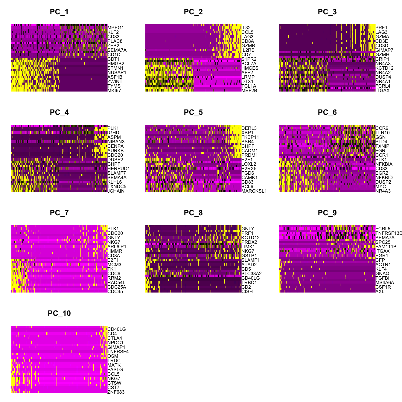

clustree(paed_sub, prefix = "RNA_snn_res.")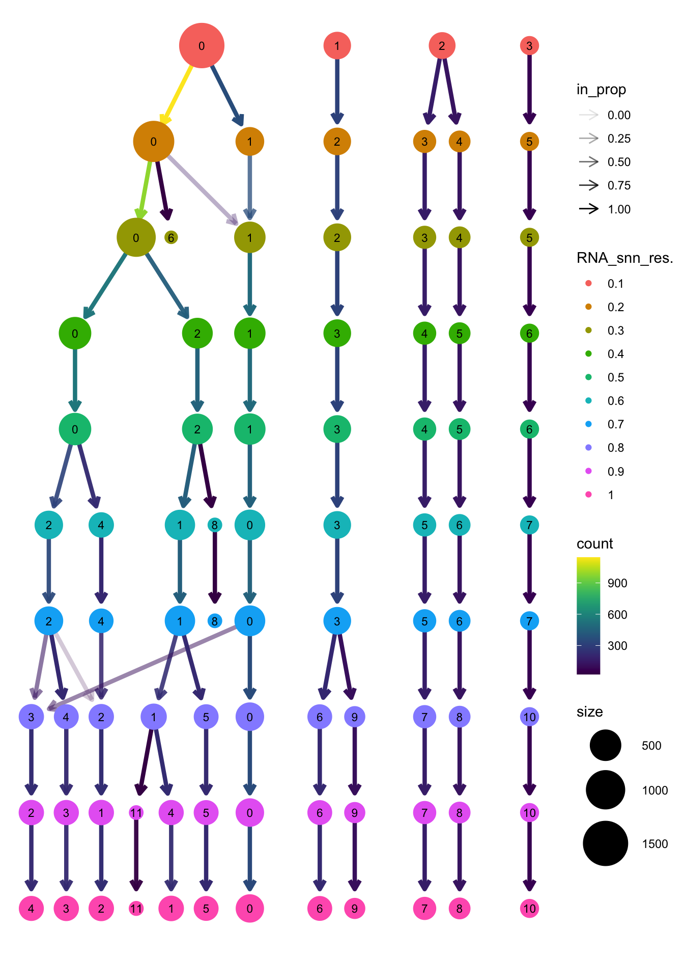

Past versions of unnamed-chunk-24-1.png

Version	Author	Date
0f07f72	Gunjan Dixit	2024-10-07

opt_res <- "RNA_snn_res.0.4"  
n <- nlevels(paed_sub$RNA_snn_res.0.4)
paed_sub$RNA_snn_res.0.4 <- factor(paed_sub$RNA_snn_res.0.4, levels = seq(0,n-1))
paed_sub$seurat_clusters <- NULL
paed_sub$cluster <- paed_sub$RNA_snn_res.0.4
Idents(paed_sub) <- paed_sub$cluster

paed_sub.markers <- FindAllMarkers(paed_sub, only.pos = TRUE, min.pct = 0.25, logfc.threshold = 0.25)

Calculating cluster 0

Calculating cluster 1

Calculating cluster 2

Calculating cluster 3

Calculating cluster 4

Calculating cluster 5

Calculating cluster 6

paed_sub.markers %>%
    group_by(cluster) %>% unique() %>% 
    top_n(n = 5, wt = avg_log2FC) -> top5

paed_sub.markers %>%
    group_by(cluster) %>% 
    slice_head(n=1) %>% 
    pull(gene) -> best.wilcox.gene.per.cluster

best.wilcox.gene.per.cluster

[1] "ITGAX" "IGHD"  "EGR3"  "MEF2B" "KIFC1" "IL32"  "HID1" 

Feature plot shows the expression of top marker genes per cluster.

FeaturePlot(paed_sub,features=best.wilcox.gene.per.cluster, reduction = 'umap.new', raster = FALSE, ncol = 2, label = TRUE)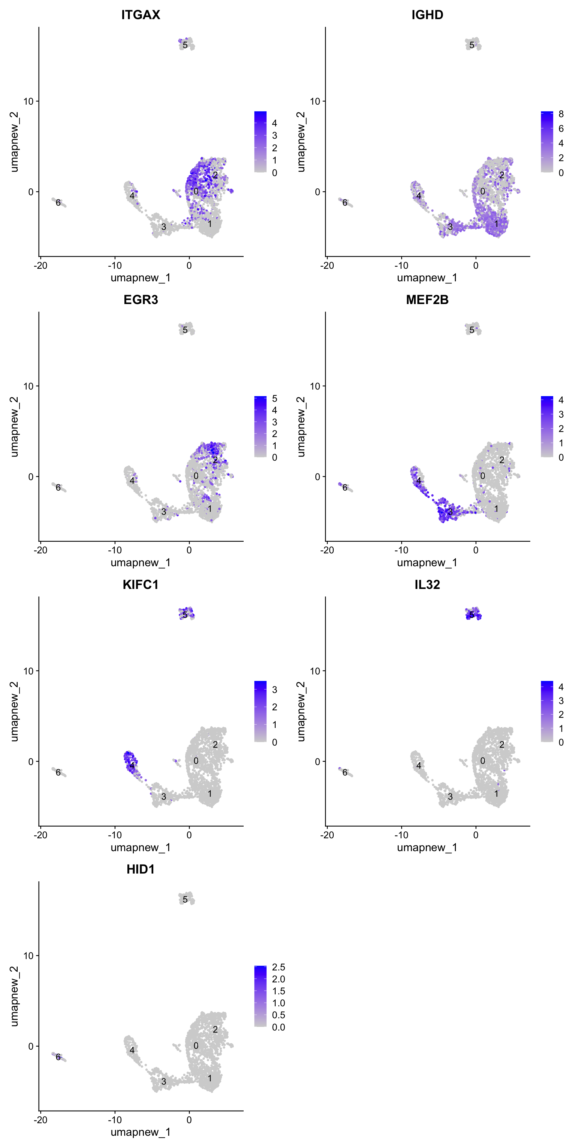

Top 10 marker genes from Seurat

## Seurat top markers
top10 <- paed_sub.markers %>%
    group_by(cluster) %>%
    top_n(n = 10, wt = avg_log2FC) %>%
    ungroup() %>%
    distinct(gene, .keep_all = TRUE) %>%
    arrange(cluster, desc(avg_log2FC))

cluster_colors <- paletteer::paletteer_d("pals::glasbey")[factor(top10$cluster)]

DotPlot(paed_sub,    
        features = unique(top10$gene),
        group.by = opt_res,
        cols = c("azure1", "blueviolet"),
        dot.scale = 3, assay = "RNA") +
    RotatedAxis() +
    FontSize(y.text = 8, x.text = 12) +
    labs(y = element_blank(), x = element_blank()) +
    coord_flip() +
    theme(axis.text.y = element_text(color = cluster_colors)) +
    ggtitle("Top 10 marker genes per cluster (Seurat)")

Warning: Vectorized input to `element_text()` is not officially supported.
ℹ Results may be unexpected or may change in future versions of ggplot2.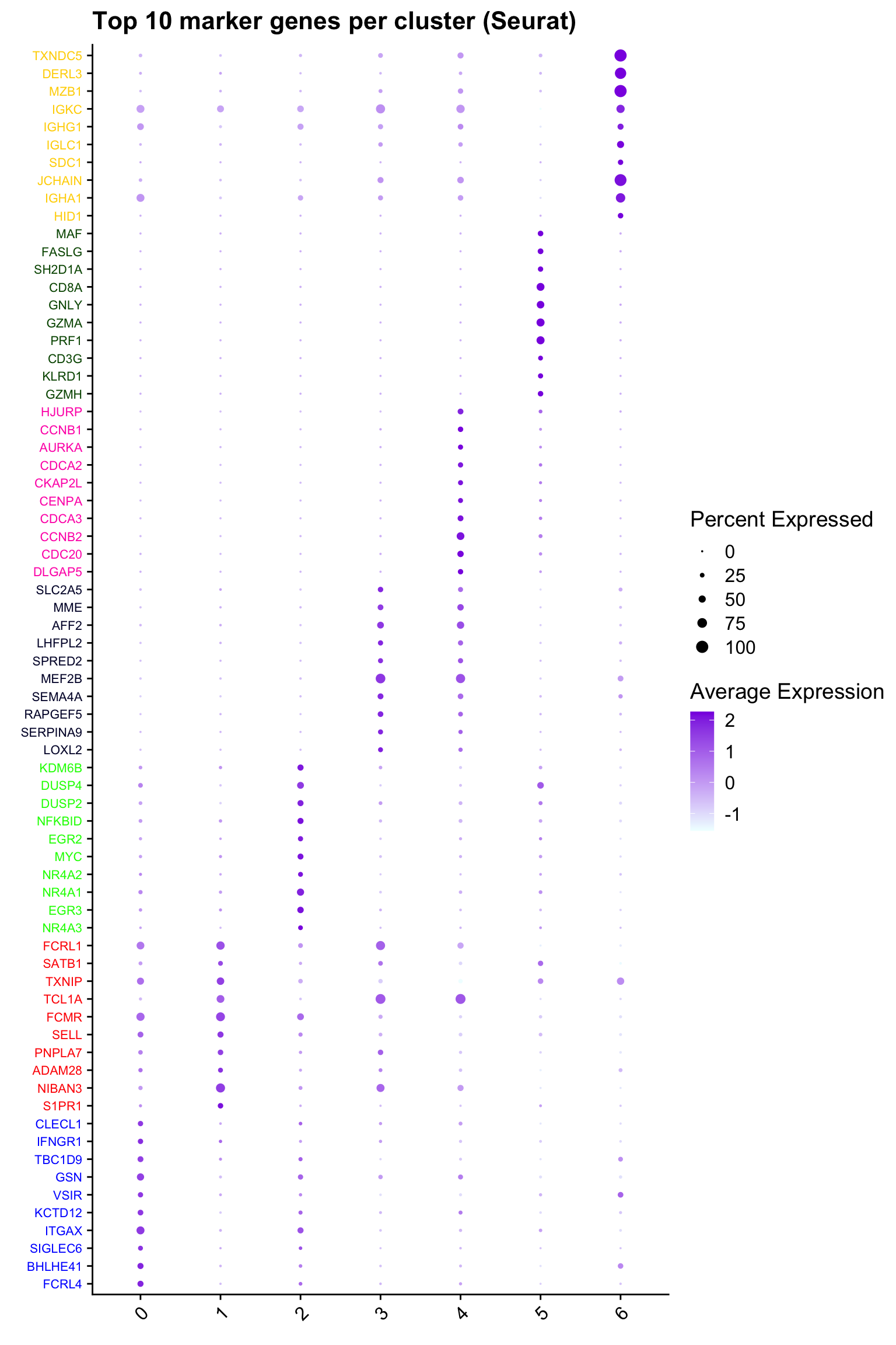

out_markers <- here("output",
            "CSV", 
            paste(tissue,"_Marker_genes_Reclustered_Bcell_population.withoutDecontX.",opt_res, sep = ""))

dir.create(out_markers, recursive = TRUE, showWarnings = FALSE)

for (cl in unique(paed_sub.markers$cluster)) {
  cluster_data <- paed_sub.markers %>% dplyr::filter(cluster == cl)
  file_name <- here(out_markers, paste0("G000231_Neeland_",tissue, "_cluster_", cl, ".csv"))
  write.csv(cluster_data, file = file_name)
}

Save subclustered SEU object

out2 <- here("output",
            "RDS", "AllBatches_Subclustering_SEUs", tissue,
             paste0("G000231_Neeland_",tissue,".Bcell_population.subclusters_without_DecontX.SEU.rds"))
#dir.create(out2)
if (!file.exists(out2)) {
  saveRDS(paed_sub, file = out2)
}

Compare two seurat objects

cl7_cells <- WhichCells(paed_sub, idents = 7)

out3 <- here("output",
            "RDS", "AllBatches_Subclustering_SEUs", tissue,
             paste0("G000231_Neeland_",tissue,".macro_population.subclusters.SEU.rds"))
paed_sub1 <- readRDS(out3)

DimPlot(paed_sub, reduction = "umap.new", group.by = "RNA_snn_res.0.7", label = TRUE, label.size = 4.5, repel = TRUE, raster = FALSE , cells.highlight = cl7_cells)
DimPlot(paed_sub1, reduction = "umap.new", group.by = "RNA_snn_res.0.7", label = TRUE, label.size = 4.5, repel = TRUE, raster = FALSE , cells.highlight = cl7_cells)

Session information

sessionInfo()

R version 4.3.2 (2023-10-31)
Platform: aarch64-apple-darwin20 (64-bit)
Running under: macOS 15.0.1

Matrix products: default
BLAS:   /Library/Frameworks/R.framework/Versions/4.3-arm64/Resources/lib/libRblas.0.dylib 
LAPACK: /Library/Frameworks/R.framework/Versions/4.3-arm64/Resources/lib/libRlapack.dylib;  LAPACK version 3.11.0

locale:
[1] en_US.UTF-8/en_US.UTF-8/en_US.UTF-8/C/en_US.UTF-8/en_US.UTF-8

time zone: Australia/Melbourne
tzcode source: internal

attached base packages:
[1] stats4    stats     graphics  grDevices utils     datasets  methods  
[8] base     

other attached packages:
 [1] readxl_1.4.3         org.Hs.eg.db_3.18.0  AnnotationDbi_1.64.1
 [4] IRanges_2.36.0       S4Vectors_0.40.2     Biobase_2.62.0      
 [7] BiocGenerics_0.48.1  speckle_1.2.0        edgeR_4.0.16        
[10] limma_3.58.1         patchwork_1.2.0      data.table_1.15.0   
[13] RColorBrewer_1.1-3   kableExtra_1.4.0     clustree_0.5.1      
[16] ggraph_2.1.0         Seurat_5.0.1.9009    SeuratObject_5.0.1  
[19] sp_2.1-3             glue_1.7.0           here_1.0.1          
[22] lubridate_1.9.3      forcats_1.0.0        stringr_1.5.1       
[25] dplyr_1.1.4          purrr_1.0.2          readr_2.1.5         
[28] tidyr_1.3.1          tibble_3.2.1         ggplot2_3.5.0       
[31] tidyverse_2.0.0      BiocStyle_2.30.0     workflowr_1.7.1     

loaded via a namespace (and not attached):
  [1] fs_1.6.3                    matrixStats_1.2.0          
  [3] spatstat.sparse_3.0-3       bitops_1.0-7               
  [5] httr_1.4.7                  tools_4.3.2                
  [7] sctransform_0.4.1           backports_1.4.1            
  [9] utf8_1.2.4                  R6_2.5.1                   
 [11] lazyeval_0.2.2              uwot_0.1.16                
 [13] withr_3.0.0                 gridExtra_2.3              
 [15] progressr_0.14.0            cli_3.6.2                  
 [17] spatstat.explore_3.2-6      fastDummies_1.7.3          
 [19] prismatic_1.1.1             labeling_0.4.3             
 [21] sass_0.4.8                  spatstat.data_3.0-4        
 [23] ggridges_0.5.6              pbapply_1.7-2              
 [25] systemfonts_1.0.5           svglite_2.1.3              
 [27] parallelly_1.37.0           rstudioapi_0.15.0          
 [29] RSQLite_2.3.5               generics_0.1.3             
 [31] ica_1.0-3                   spatstat.random_3.2-2      
 [33] Matrix_1.6-5                ggbeeswarm_0.7.2           
 [35] fansi_1.0.6                 abind_1.4-5                
 [37] lifecycle_1.0.4             whisker_0.4.1              
 [39] yaml_2.3.8                  SummarizedExperiment_1.32.0
 [41] SparseArray_1.2.4           Rtsne_0.17                 
 [43] paletteer_1.6.0             grid_4.3.2                 
 [45] blob_1.2.4                  promises_1.2.1             
 [47] crayon_1.5.2                miniUI_0.1.1.1             
 [49] lattice_0.22-5              cowplot_1.1.3              
 [51] KEGGREST_1.42.0             pillar_1.9.0               
 [53] knitr_1.45                  GenomicRanges_1.54.1       
 [55] future.apply_1.11.1         codetools_0.2-19           
 [57] leiden_0.4.3.1              getPass_0.2-4              
 [59] vctrs_0.6.5                 png_0.1-8                  
 [61] spam_2.10-0                 cellranger_1.1.0           
 [63] gtable_0.3.4                rematch2_2.1.2             
 [65] cachem_1.0.8                xfun_0.42                  
 [67] S4Arrays_1.2.0              mime_0.12                  
 [69] tidygraph_1.3.1             survival_3.5-8             
 [71] SingleCellExperiment_1.24.0 statmod_1.5.0              
 [73] ellipsis_0.3.2              fitdistrplus_1.1-11        
 [75] ROCR_1.0-11                 nlme_3.1-164               
 [77] bit64_4.0.5                 RcppAnnoy_0.0.22           
 [79] GenomeInfoDb_1.38.6         rprojroot_2.0.4            
 [81] bslib_0.6.1                 irlba_2.3.5.1              
 [83] vipor_0.4.7                 KernSmooth_2.23-22         
 [85] colorspace_2.1-0            DBI_1.2.2                  
 [87] ggrastr_1.0.2               tidyselect_1.2.0           
 [89] processx_3.8.3              bit_4.0.5                  
 [91] compiler_4.3.2              git2r_0.33.0               
 [93] xml2_1.3.6                  DelayedArray_0.28.0        
 [95] plotly_4.10.4               checkmate_2.3.1            
 [97] scales_1.3.0                lmtest_0.9-40              
 [99] callr_3.7.5                 digest_0.6.34              
[101] goftest_1.2-3               spatstat.utils_3.0-4       
[103] presto_1.0.0                rmarkdown_2.25             
[105] XVector_0.42.0              htmltools_0.5.7            
[107] pkgconfig_2.0.3             MatrixGenerics_1.14.0      
[109] highr_0.10                  fastmap_1.1.1              
[111] rlang_1.1.3                 htmlwidgets_1.6.4          
[113] shiny_1.8.0                 farver_2.1.1               
[115] jquerylib_0.1.4             zoo_1.8-12                 
[117] jsonlite_1.8.8              RCurl_1.98-1.14            
[119] magrittr_2.0.3              GenomeInfoDbData_1.2.11    
[121] dotCall64_1.1-1             munsell_0.5.0              
[123] Rcpp_1.0.12                 viridis_0.6.5              
[125] reticulate_1.35.0           stringi_1.8.3              
[127] zlibbioc_1.48.0             MASS_7.3-60.0.1            
[129] plyr_1.8.9                  parallel_4.3.2             
[131] listenv_0.9.1               ggrepel_0.9.5              
[133] deldir_2.0-2                Biostrings_2.70.2          
[135] graphlayouts_1.1.0          splines_4.3.2              
[137] tensor_1.5                  hms_1.1.3                  
[139] locfit_1.5-9.8              ps_1.7.6                   
[141] igraph_2.0.2                spatstat.geom_3.2-8        
[143] RcppHNSW_0.6.0              reshape2_1.4.4             
[145] evaluate_0.23               BiocManager_1.30.22        
[147] tzdb_0.4.0                  tweenr_2.0.3               
[149] httpuv_1.6.14               RANN_2.6.1                 
[151] polyclip_1.10-6             future_1.33.1              
[153] scattermore_1.2             ggforce_0.4.2              
[155] xtable_1.8-4                RSpectra_0.16-1            
[157] later_1.3.2                 viridisLite_0.4.2          
[159] beeswarm_0.4.0              memoise_2.0.1              
[161] cluster_2.1.6               timechange_0.3.0           
[163] globals_0.16.2