Bronchial_brushings
Clustering and Marker gene analysis
Gunjan Dixit
July 26, 2024
Last updated: 2024-07-26
Checks: 6 1
Knit directory: paed-airway-allTissues/
This reproducible R Markdown analysis was created with workflowr (version 1.7.1). The Checks tab describes the reproducibility checks that were applied when the results were created. The Past versions tab lists the development history.
The R Markdown file has unstaged changes. To know which version of
the R Markdown file created these results, you’ll want to first commit
it to the Git repo. If you’re still working on the analysis, you can
ignore this warning. When you’re finished, you can run
wflow_publish to commit the R Markdown file and build the
HTML.
Great job! The global environment was empty. Objects defined in the global environment can affect the analysis in your R Markdown file in unknown ways. For reproduciblity it’s best to always run the code in an empty environment.
The command set.seed(20230811) was run prior to running
the code in the R Markdown file. Setting a seed ensures that any results
that rely on randomness, e.g. subsampling or permutations, are
reproducible.
Great job! Recording the operating system, R version, and package versions is critical for reproducibility.
Nice! There were no cached chunks for this analysis, so you can be confident that you successfully produced the results during this run.
Great job! Using relative paths to the files within your workflowr project makes it easier to run your code on other machines.
Great! You are using Git for version control. Tracking code development and connecting the code version to the results is critical for reproducibility.
The results in this page were generated with repository version cedb23d. See the Past versions tab to see a history of the changes made to the R Markdown and HTML files.
Note that you need to be careful to ensure that all relevant files for
the analysis have been committed to Git prior to generating the results
(you can use wflow_publish or
wflow_git_commit). workflowr only checks the R Markdown
file, but you know if there are other scripts or data files that it
depends on. Below is the status of the Git repository when the results
were generated:
Ignored files:
    Ignored:    .DS_Store
    Ignored:    .RData
    Ignored:    .Rhistory
    Ignored:    .Rproj.user/
    Ignored:    analysis/.DS_Store
    Ignored:    data/.DS_Store
    Ignored:    data/RDS/
    Ignored:    output/.DS_Store
    Ignored:    output/CSV/.DS_Store
    Ignored:    output/G000231_Neeland_batch1/
    Ignored:    output/G000231_Neeland_batch2_1/
    Ignored:    output/G000231_Neeland_batch2_2/
    Ignored:    output/G000231_Neeland_batch3/
    Ignored:    output/G000231_Neeland_batch4/
    Ignored:    output/G000231_Neeland_batch5/
    Ignored:    output/G000231_Neeland_batch9_1/
    Ignored:    output/RDS/
    Ignored:    output/plots/

Untracked files:
    Untracked:  VennDiagram.2024-07-24_11-48-08.297746.log
    Untracked:  VennDiagram.2024-07-24_12-25-12.854839.log
    Untracked:  VennDiagram.2024-07-24_12-25-22.005094.log
    Untracked:  VennDiagram.2024-07-24_12-29-34.757841.log
    Untracked:  analysis/03_Batch_Integration.Rmd
    Untracked:  analysis/Age_proportions.Rmd
    Untracked:  analysis/Age_proportions_AllBatches.Rmd
    Untracked:  analysis/Batch_Integration_&_Downstream_analysis.Rmd
    Untracked:  analysis/Batch_correction_&_Downstream.Rmd
    Untracked:  analysis/Cell_cycle_regression.Rmd
    Untracked:  analysis/Preprocessing_Batch1_Nasal_brushings.Rmd
    Untracked:  analysis/Preprocessing_Batch2_Tonsils.Rmd
    Untracked:  analysis/Preprocessing_Batch3_Adenoids.Rmd
    Untracked:  analysis/Preprocessing_Batch4_Bronchial_brushings.Rmd
    Untracked:  analysis/Preprocessing_Batch5_Nasal_brushings.Rmd
    Untracked:  analysis/Preprocessing_Batch6_BAL.Rmd
    Untracked:  analysis/Preprocessing_Batch7_Bronchial_brushings.Rmd
    Untracked:  analysis/Preprocessing_Batch8_Adenoids.Rmd
    Untracked:  analysis/Preprocessing_Batch9_Tonsils.Rmd
    Untracked:  analysis/VennDiagram.2024-07-24_11-54-23.569848.log
    Untracked:  analysis/VennDiagram.2024-07-24_11-55-06.582353.log
    Untracked:  analysis/VennDiagram.2024-07-24_12-28-47.017253.log
    Untracked:  analysis/VennDiagram.2024-07-24_12-33-05.913419.log
    Untracked:  analysis/VennDiagram.2024-07-24_13-42-31.593316.log
    Untracked:  analysis/cell_cycle_regression.R
    Untracked:  analysis/test.Rmd
    Untracked:  analysis/testing_age_all.Rmd
    Untracked:  data/Cell_labels_Mel/
    Untracked:  data/Cell_labels_Mel_v2/
    Untracked:  data/Hs.c2.cp.reactome.v7.1.entrez.rds
    Untracked:  data/Raw_feature_bc_matrix/
    Untracked:  data/celltypes_Mel_GD_v3.xlsx
    Untracked:  data/celltypes_Mel_GD_v4_no_dups.xlsx
    Untracked:  data/celltypes_Mel_modified.xlsx
    Untracked:  data/celltypes_Mel_v2.csv
    Untracked:  data/celltypes_Mel_v2.xlsx
    Untracked:  data/celltypes_Mel_v2_MN.xlsx
    Untracked:  data/celltypes_for_mel_MN.xlsx
    Untracked:  data/earlyAIR_sample_sheets_combined.xlsx
    Untracked:  output/CSV/Bronchial_brushings_Marker_gene_clusters.limmaTrendRNA_snn_res.0.4/
    Untracked:  stacked_barplot.png
    Untracked:  stacked_barplot_donor_id.png

Unstaged changes:
    Deleted:    02_QC_exploratoryPlots.Rmd
    Deleted:    02_QC_exploratoryPlots.html
    Modified:   analysis/00_AllBatches_overview.Rmd
    Modified:   analysis/01_QC_emptyDrops.Rmd
    Modified:   analysis/02_QC_exploratoryPlots.Rmd
    Modified:   analysis/Age_modeling.Rmd
    Modified:   analysis/AllBatches_QCExploratory.Rmd
    Modified:   analysis/BAL.Rmd
    Modified:   analysis/Bronchial_brushings.Rmd
    Modified:   analysis/Nasal_brushings.Rmd
    Modified:   output/CSV/BAL_Marker_gene_clusters.limmaTrendRNA_snn_res.0.4/REACTOME-cluster-limma-c0.csv
    Modified:   output/CSV/BAL_Marker_gene_clusters.limmaTrendRNA_snn_res.0.4/REACTOME-cluster-limma-c1.csv
    Modified:   output/CSV/BAL_Marker_gene_clusters.limmaTrendRNA_snn_res.0.4/REACTOME-cluster-limma-c10.csv
    Modified:   output/CSV/BAL_Marker_gene_clusters.limmaTrendRNA_snn_res.0.4/REACTOME-cluster-limma-c11.csv
    Modified:   output/CSV/BAL_Marker_gene_clusters.limmaTrendRNA_snn_res.0.4/REACTOME-cluster-limma-c12.csv
    Modified:   output/CSV/BAL_Marker_gene_clusters.limmaTrendRNA_snn_res.0.4/REACTOME-cluster-limma-c13.csv
    Modified:   output/CSV/BAL_Marker_gene_clusters.limmaTrendRNA_snn_res.0.4/REACTOME-cluster-limma-c14.csv
    Modified:   output/CSV/BAL_Marker_gene_clusters.limmaTrendRNA_snn_res.0.4/REACTOME-cluster-limma-c15.csv
    Modified:   output/CSV/BAL_Marker_gene_clusters.limmaTrendRNA_snn_res.0.4/REACTOME-cluster-limma-c16.csv
    Modified:   output/CSV/BAL_Marker_gene_clusters.limmaTrendRNA_snn_res.0.4/REACTOME-cluster-limma-c17.csv
    Modified:   output/CSV/BAL_Marker_gene_clusters.limmaTrendRNA_snn_res.0.4/REACTOME-cluster-limma-c2.csv
    Modified:   output/CSV/BAL_Marker_gene_clusters.limmaTrendRNA_snn_res.0.4/REACTOME-cluster-limma-c3.csv
    Modified:   output/CSV/BAL_Marker_gene_clusters.limmaTrendRNA_snn_res.0.4/REACTOME-cluster-limma-c4.csv
    Modified:   output/CSV/BAL_Marker_gene_clusters.limmaTrendRNA_snn_res.0.4/REACTOME-cluster-limma-c5.csv
    Modified:   output/CSV/BAL_Marker_gene_clusters.limmaTrendRNA_snn_res.0.4/REACTOME-cluster-limma-c6.csv
    Modified:   output/CSV/BAL_Marker_gene_clusters.limmaTrendRNA_snn_res.0.4/REACTOME-cluster-limma-c7.csv
    Modified:   output/CSV/BAL_Marker_gene_clusters.limmaTrendRNA_snn_res.0.4/REACTOME-cluster-limma-c8.csv
    Modified:   output/CSV/BAL_Marker_gene_clusters.limmaTrendRNA_snn_res.0.4/REACTOME-cluster-limma-c9.csv
    Modified:   output/CSV/BAL_Marker_gene_clusters.limmaTrendRNA_snn_res.0.4/up-cluster-limma-c0.csv
    Modified:   output/CSV/BAL_Marker_gene_clusters.limmaTrendRNA_snn_res.0.4/up-cluster-limma-c1.csv
    Modified:   output/CSV/BAL_Marker_gene_clusters.limmaTrendRNA_snn_res.0.4/up-cluster-limma-c10.csv
    Modified:   output/CSV/BAL_Marker_gene_clusters.limmaTrendRNA_snn_res.0.4/up-cluster-limma-c11.csv
    Modified:   output/CSV/BAL_Marker_gene_clusters.limmaTrendRNA_snn_res.0.4/up-cluster-limma-c12.csv
    Modified:   output/CSV/BAL_Marker_gene_clusters.limmaTrendRNA_snn_res.0.4/up-cluster-limma-c13.csv
    Modified:   output/CSV/BAL_Marker_gene_clusters.limmaTrendRNA_snn_res.0.4/up-cluster-limma-c14.csv
    Modified:   output/CSV/BAL_Marker_gene_clusters.limmaTrendRNA_snn_res.0.4/up-cluster-limma-c15.csv
    Modified:   output/CSV/BAL_Marker_gene_clusters.limmaTrendRNA_snn_res.0.4/up-cluster-limma-c16.csv
    Modified:   output/CSV/BAL_Marker_gene_clusters.limmaTrendRNA_snn_res.0.4/up-cluster-limma-c17.csv
    Modified:   output/CSV/BAL_Marker_gene_clusters.limmaTrendRNA_snn_res.0.4/up-cluster-limma-c2.csv
    Modified:   output/CSV/BAL_Marker_gene_clusters.limmaTrendRNA_snn_res.0.4/up-cluster-limma-c3.csv
    Modified:   output/CSV/BAL_Marker_gene_clusters.limmaTrendRNA_snn_res.0.4/up-cluster-limma-c4.csv
    Modified:   output/CSV/BAL_Marker_gene_clusters.limmaTrendRNA_snn_res.0.4/up-cluster-limma-c5.csv
    Modified:   output/CSV/BAL_Marker_gene_clusters.limmaTrendRNA_snn_res.0.4/up-cluster-limma-c6.csv
    Modified:   output/CSV/BAL_Marker_gene_clusters.limmaTrendRNA_snn_res.0.4/up-cluster-limma-c7.csv
    Modified:   output/CSV/BAL_Marker_gene_clusters.limmaTrendRNA_snn_res.0.4/up-cluster-limma-c8.csv
    Modified:   output/CSV/BAL_Marker_gene_clusters.limmaTrendRNA_snn_res.0.4/up-cluster-limma-c9.csv
Note that any generated files, e.g. HTML, png, CSS, etc., are not included in this status report because it is ok for generated content to have uncommitted changes.
These are the previous versions of the repository in which changes were
made to the R Markdown (analysis/Bronchial_brushings.Rmd)
and HTML (docs/Bronchial_brushings.html) files. If you’ve
configured a remote Git repository (see ?wflow_git_remote),
click on the hyperlinks in the table below to view the files as they
were in that past version.
| File | Version | Author | Date | Message |
|---|---|---|---|---|
| Rmd | c20f60f | Gunjan Dixit | 2024-07-08 | Updated marker gene dot plots |
| html | c20f60f | Gunjan Dixit | 2024-07-08 | Updated marker gene dot plots |
| Rmd | 77c742e | Gunjan Dixit | 2024-06-26 | Updated RMarkdown files of all Tissues |
| html | 77c742e | Gunjan Dixit | 2024-06-26 | Updated RMarkdown files of all Tissues |
| Rmd | a94371e | Gunjan Dixit | 2024-06-07 | Reclustering analysis |
| html | a94371e | Gunjan Dixit | 2024-06-07 | Reclustering analysis |
| Rmd | e0e83af | Gunjan Dixit | 2024-06-04 | Updated reclustering |
| html | e0e83af | Gunjan Dixit | 2024-06-04 | Updated reclustering |
| Rmd | 320ccbd | Gunjan Dixit | 2024-05-01 | Modified/Annotated RMarkdown files |
| html | 320ccbd | Gunjan Dixit | 2024-05-01 | Modified/Annotated RMarkdown files |
| html | f460bd0 | Gunjan Dixit | 2024-04-26 | Modified BAL |
| Rmd | 9492583 | Gunjan Dixit | 2024-04-26 | Added new analysis |
| html | 9492583 | Gunjan Dixit | 2024-04-26 | Added new analysis |
Introduction
This Rmarkdown file loads and analyzes the Seurat object for
Bronchial Brushings (Batch4). It performs clustering at
various resolutions ranging from 0-1, followed by visualization of
identified clusters and Broad Level 3 cell labels on UMAP. Next, the
FindAllMarkers function is used to perform marker gene
analysis to identify marker genes for each cluster. The top marker gene
is visualized using FeaturePlot, ViolinPlot
and Heatmap. The identified marker genes are stored in CSV
format for each cluster at the optimum resolution identified using
clustree function.
Load libraries
suppressPackageStartupMessages({
  library(BiocStyle)
  library(tidyverse)
  library(here)
  library(glue)
  library(dplyr)
  library(Seurat)
  library(clustree)
  library(kableExtra)
  library(RColorBrewer)
  library(data.table)
  library(ggplot2)
  library(patchwork)
  library(limma)
  library(edgeR)
  library(speckle)
  library(AnnotationDbi)
  library(org.Hs.eg.db)
})
Load Input data
For Bronchial brushings, we used only Batch4 for the downstream analysis.
tissue <- "Bronchial_brushings"
out <- here("output/RDS/AllBatches_Harmony_SEUs/G000231_Neeland_Bronchial_brushings.clusters.SEU.rds")
seu_obj <- readRDS(out)
seu_obj
An object of class Seurat
18046 features across 33917 samples within 1 assay
Active assay: RNA (18046 features, 2000 variable features)
3 layers present: counts, data, scale.data
3 dimensional reductions calculated: pca, umap, umap.unintegratedClustering
Clustering is done on the “harmony” or batch integrated reduction at resolutions ranging from 0-1.
out1 <- here("output",
            "RDS", "AllBatches_Clustering_SEUs",
             paste0("G000231_Neeland_",tissue,".Clusters.SEU.rds"))
#dir.create(out1)

resolutions <- seq(0.1, 1, by = 0.1)
if (!file.exists(out1)) {
seu_obj <- FindNeighbors(seu_obj, reduction = "pca", dims = 1:30)
seu_obj <- FindClusters(seu_obj, resolution = seq(0.1, 1, by = 0.1), algorithm = 3)
saveRDS(seu_obj, file = out1)
} else {
    seu_obj <- readRDS(out1)
}
The clustree function is used to visualize the
clustering at different resolutions to identify the most optimum
resolution.
clustree(seu_obj, prefix = "RNA_snn_res.")
| Version | Author | Date |
|---|---|---|
| 9492583 | Gunjan Dixit | 2024-04-26 |
Based on the clustering tree, we chose an intermediate/optimum resolution where the clustering results are the most stable, with the least amount of shuffling cells.
opt_res <- "RNA_snn_res.0.4"
n <- nlevels(seu_obj$RNA_snn_res.0.4)
seu_obj$RNA_snn_res.0.4 <- factor(seu_obj$RNA_snn_res.0.4, levels = seq(0,n-1))
seu_obj$seurat_clusters <- NULL
seu_obj$cluster <- seu_obj$RNA_snn_res.0.4
Idents(seu_obj) <- seu_obj$cluster
UMAP after clustering
Defining colours for each cell-type to be consistent with other age-related/cell type composition plots.
my_colors <- c(
  "B cells" = "steelblue",
  "CD4 T cells" = "brown",
  "Double negative T cells" = "gold",
  "CD8 T cells" = "lightgreen",
  "Pre B/T cells" = "orchid",
  "Innate lymphoid cells" = "tan",
  "Natural Killer cells" = "blueviolet",
  "Macrophages" = "green4",
  "Cycling T cells" = "turquoise",
  "Dendritic cells" = "grey80",
  "Gamma delta T cells" = "mediumvioletred",
  "Epithelial lineage" = "darkorange",
  "Granulocytes" = "olivedrab",
  "Fibroblast lineage" = "lavender",
  "None" = "white",
  "Monocytes" = "peachpuff",
  "Endothelial lineage" = "cadetblue",
  "SMG duct" = "lightpink",
  "Neuroendocrine" = "skyblue",
  "Doublet query/Other" = "#d62728"
)
UMAP displaying clusters at opt_res resolution and Broad
cell Labels Level 3.
p1 <- DimPlot(seu_obj, reduction = "umap", raster = FALSE ,repel = TRUE, label = TRUE,label.size = 3.5, group.by = opt_res) +  NoLegend()

p2 <- DimPlot(seu_obj, reduction = "umap", raster = FALSE, repel = TRUE, label = TRUE, label.size = 3.5, group.by = "Broad_cell_label_3") + NoLegend() +
  scale_colour_manual(values = my_colors) +
  ggtitle(paste0(tissue, ": UMAP"))


p1 / p2 
| Version | Author | Date |
|---|---|---|
| 9492583 | Gunjan Dixit | 2024-04-26 |
Save batch corrected Object
out1 <- here("output",
            "RDS", "AllBatches_Clustering_SEUs",
             paste0("G000231_Neeland_",tissue,".Clusters.SEU.rds"))
#dir.create(out1)
if (!file.exists(out1)) {
  saveRDS(seu_obj, file = out1)
}
Marker Gene Analysis
#seu_obj <- JoinLayers(seu_obj)
paed.markers <- FindAllMarkers(seu_obj, only.pos = TRUE, min.pct = 0.25, logfc.threshold = 0.25)
Extracting top 5 genes per cluster for visualization. The ‘top5’ contains the top 5 genes with the highest weighted average avg_log2FC within each cluster and the ‘best.wilcox.gene.per.cluster’ contains the single best gene with the highest weighted average avg_log2FC for each cluster.
paed.markers %>%
    group_by(cluster) %>% unique() %>%
    top_n(n = 5, wt = avg_log2FC) -> top5

paed.markers %>%
    group_by(cluster) %>%
    slice_head(n=1) %>%
    pull(gene) -> best.wilcox.gene.per.cluster

best.wilcox.gene.per.cluster
[1] "FABP4" "CCL5" "KRT7" "LILRB2" "CFAP43" "CD79A" "CTXN1" "PPIL6"
[9] "SPOCK2" "CSF3R" "ADH1C" "APOE" "CPA3" "UHRF1" "LILRA4" "ASCL3"
[17] "KRT13" "MZB1" Marker gene expression in clusters
This heatmap depicts the expression of top five genes in each cluster.
DoHeatmap(seu_obj, features = top5$gene) + NoLegend()
| Version | Author | Date |
|---|---|---|
| 320ccbd | Gunjan Dixit | 2024-05-01 |
Violin plot shows the expression of top marker gene per cluster.
VlnPlot(seu_obj, features=best.wilcox.gene.per.cluster, ncol = 2, raster = FALSE, pt.size = FALSE)
| Version | Author | Date |
|---|---|---|
| 320ccbd | Gunjan Dixit | 2024-05-01 |
Feature plot shows the expression of top marker genes per cluster.
FeaturePlot(seu_obj,features=best.wilcox.gene.per.cluster, reduction = 'umap', raster = FALSE, ncol = 2)
| Version | Author | Date |
|---|---|---|
| 320ccbd | Gunjan Dixit | 2024-05-01 |
Extract markers for each cluster
This section extracts marker genes for each cluster and save them as a CSV file.
out_markers <- here("output",
            "CSV",
            paste(tissue,"_Marker_gene_clusters.",opt_res, sep = ""))

dir.create(out_markers, recursive = TRUE, showWarnings = FALSE)

for (cl in unique(paed.markers$cluster)) {
  cluster_data <- paed.markers %>% dplyr::filter(cluster == cl)
  file_name <- here(out_markers, paste0("G000231_Neeland_",tissue, "_cluster_", cl, ".csv"))
  write.csv(cluster_data, file = file_name)
}
Updated cell-type labels
cell_labels <- readxl::read_excel(here("data/Cell_labels_Mel/earlyAIR_bronchial_brushing_annotations_02.05.24_update.xlsx"))
new_cluster_names <- cell_labels %>%
  dplyr::select(cluster, annotation) %>%
  deframe()

seu_obj <- RenameIdents(seu_obj, new_cluster_names)
seu_obj@meta.data$cell_labels <- Idents(seu_obj)

p3 <- DimPlot(seu_obj, reduction = "umap", raster = FALSE, repel = TRUE, label = TRUE, label.size = 3.5) + ggtitle(paste0(tissue, ": UMAP with Updated cell types"))

#p1
p3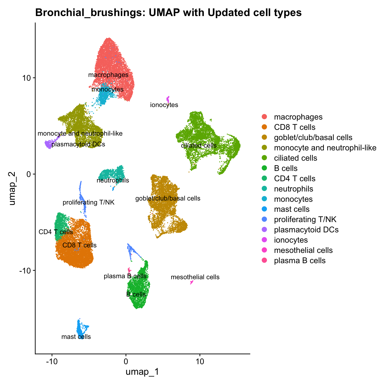
seu_obj@meta.data %>%
  ggplot(aes(x = cell_labels, fill = cell_labels)) +
  geom_bar() +
  geom_text(aes(label = ..count..), stat = "count",
            vjust = -0.5, colour = "black", size = 2) +
  theme(axis.text.x = element_text(angle = 90, vjust = 0.5, hjust = 1)) +
  NoLegend() + ggtitle(paste0(tissue, " : Counts per cell-type"))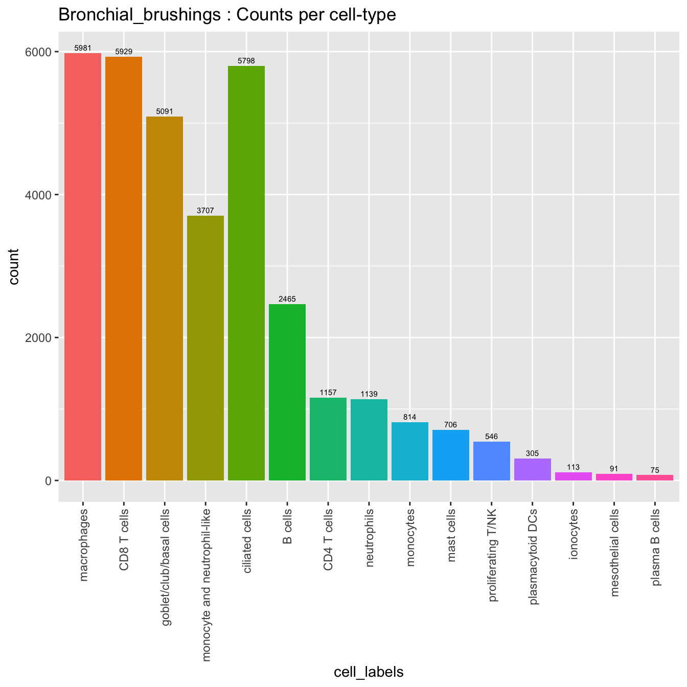
Recluster Goblet/club/Basal cells
The marker genes for this reclustering can be found here-
Subset clusters representing goblet/basal/club cells.
idx <- which(Idents(seu_obj) %in% "goblet/club/basal cells")
paed_sub <- seu_obj[,idx]
mito_genes <- grep("^MT-", rownames(paed_sub), value = TRUE)
paed_sub <- subset(paed_sub, features = setdiff(rownames(paed_sub), mito_genes))
paed_sub
An object of class Seurat
18035 features across 5091 samples within 1 assay
Active assay: RNA (18035 features, 1995 variable features)
3 layers present: counts, data, scale.data
3 dimensional reductions calculated: pca, umap, umap.unintegratedExploring clusters at resolution 0.01 to 0.1
paed_sub <- paed_sub %>%
  NormalizeData() %>%
  FindVariableFeatures() %>%
  ScaleData() %>%
  RunPCA()

paed_sub <- RunUMAP(paed_sub, dims = 1:30, reduction = "pca", reduction.name = "umap.new")

meta_data <- colnames(paed_sub@meta.data)
drop <- grep("^RNA_snn_res", meta_data, value = TRUE)
paed_sub@meta.data <- paed_sub@meta.data[, !(colnames(paed_sub@meta.data) %in% drop)]


resolutions <- seq(0.01, 0.1, by = 0.01)
paed_sub <- FindNeighbors(paed_sub, reduction = "pca", dims = 1:30)
paed_sub <- FindClusters(paed_sub, resolution = resolutions, algorithm = 3)
Modularity Optimizer version 1.3.0 by Ludo Waltman and Nees Jan van Eck
Number of nodes: 5091
Number of edges: 186471
Running smart local moving algorithm...
Maximum modularity in 10 random starts: 0.9900
Number of communities: 1
Elapsed time: 2 seconds
Modularity Optimizer version 1.3.0 by Ludo Waltman and Nees Jan van Eck
Number of nodes: 5091
Number of edges: 186471
Running smart local moving algorithm...
Maximum modularity in 10 random starts: 0.9805
Number of communities: 2
Elapsed time: 2 seconds
Modularity Optimizer version 1.3.0 by Ludo Waltman and Nees Jan van Eck
Number of nodes: 5091
Number of edges: 186471
Running smart local moving algorithm...
Maximum modularity in 10 random starts: 0.9735
Number of communities: 2
Elapsed time: 2 seconds
Modularity Optimizer version 1.3.0 by Ludo Waltman and Nees Jan van Eck
Number of nodes: 5091
Number of edges: 186471
Running smart local moving algorithm...
Maximum modularity in 10 random starts: 0.9665
Number of communities: 2
Elapsed time: 2 seconds
Modularity Optimizer version 1.3.0 by Ludo Waltman and Nees Jan van Eck
Number of nodes: 5091
Number of edges: 186471
Running smart local moving algorithm...
Maximum modularity in 10 random starts: 0.9601
Number of communities: 3
Elapsed time: 2 seconds
Modularity Optimizer version 1.3.0 by Ludo Waltman and Nees Jan van Eck
Number of nodes: 5091
Number of edges: 186471
Running smart local moving algorithm...
Maximum modularity in 10 random starts: 0.9555
Number of communities: 3
Elapsed time: 2 seconds
Modularity Optimizer version 1.3.0 by Ludo Waltman and Nees Jan van Eck
Number of nodes: 5091
Number of edges: 186471
Running smart local moving algorithm...
Maximum modularity in 10 random starts: 0.9509
Number of communities: 4
Elapsed time: 2 seconds
Modularity Optimizer version 1.3.0 by Ludo Waltman and Nees Jan van Eck
Number of nodes: 5091
Number of edges: 186471
Running smart local moving algorithm...
Maximum modularity in 10 random starts: 0.9462
Number of communities: 4
Elapsed time: 2 seconds
Modularity Optimizer version 1.3.0 by Ludo Waltman and Nees Jan van Eck
Number of nodes: 5091
Number of edges: 186471
Running smart local moving algorithm...
Maximum modularity in 10 random starts: 0.9417
Number of communities: 4
Elapsed time: 2 seconds
Modularity Optimizer version 1.3.0 by Ludo Waltman and Nees Jan van Eck
Number of nodes: 5091
Number of edges: 186471
Running smart local moving algorithm...
Maximum modularity in 10 random starts: 0.9374
Number of communities: 5
Elapsed time: 1 secondsDimHeatmap(paed_sub, dims = 1:10, cells = 500, balanced = TRUE)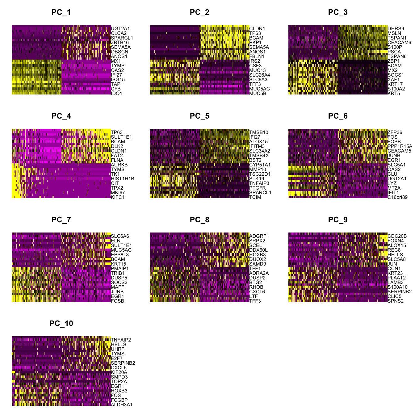
| Version | Author | Date |
|---|---|---|
| e0e83af | Gunjan Dixit | 2024-06-04 |
clustree(paed_sub, prefix = "RNA_snn_res.")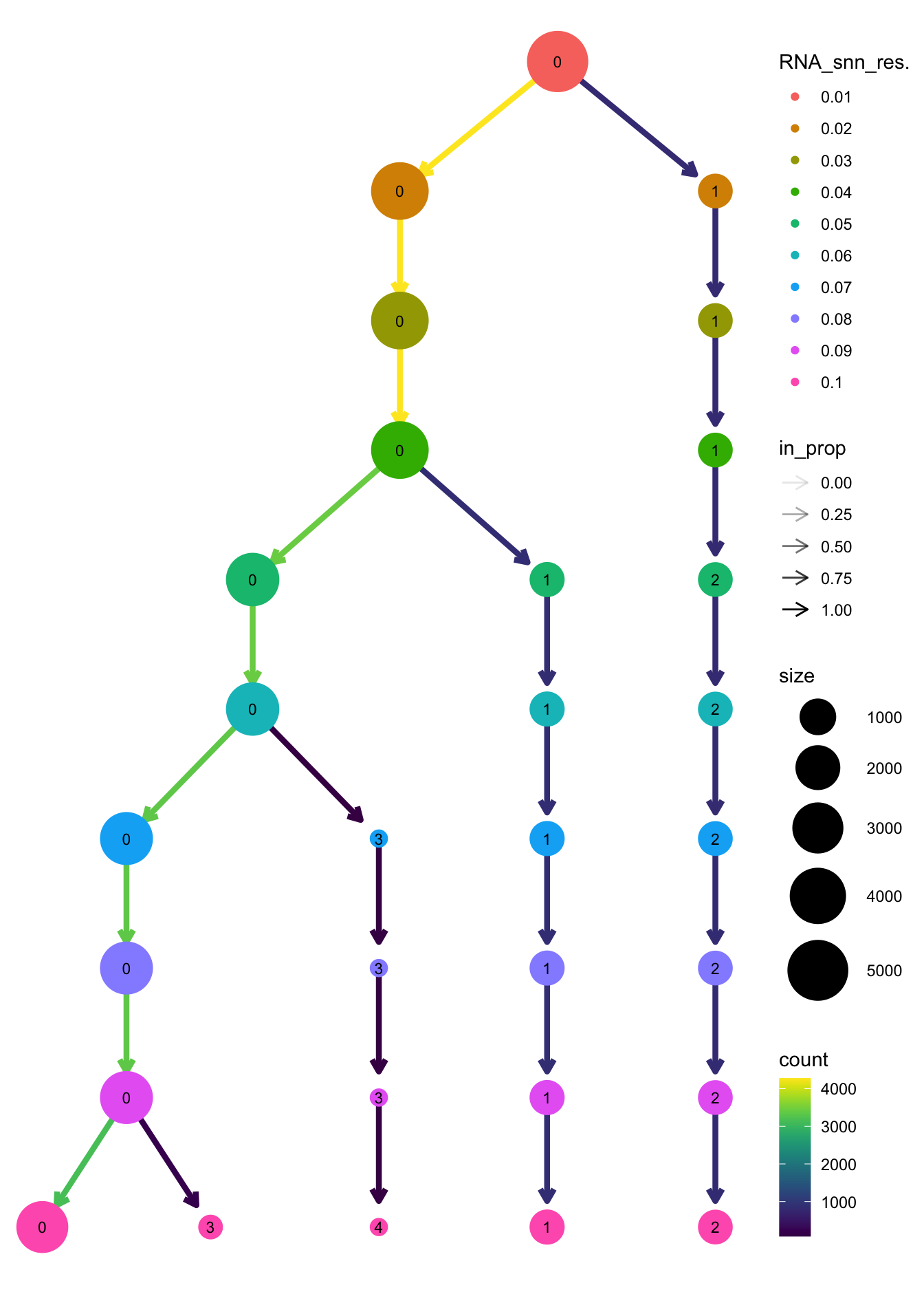
| Version | Author | Date |
|---|---|---|
| a94371e | Gunjan Dixit | 2024-06-07 |
DimPlot(paed_sub, reduction = "umap.new", group.by = "RNA_snn_res.0.05" , label = TRUE, label.size = 4.5, repel = TRUE, raster = FALSE )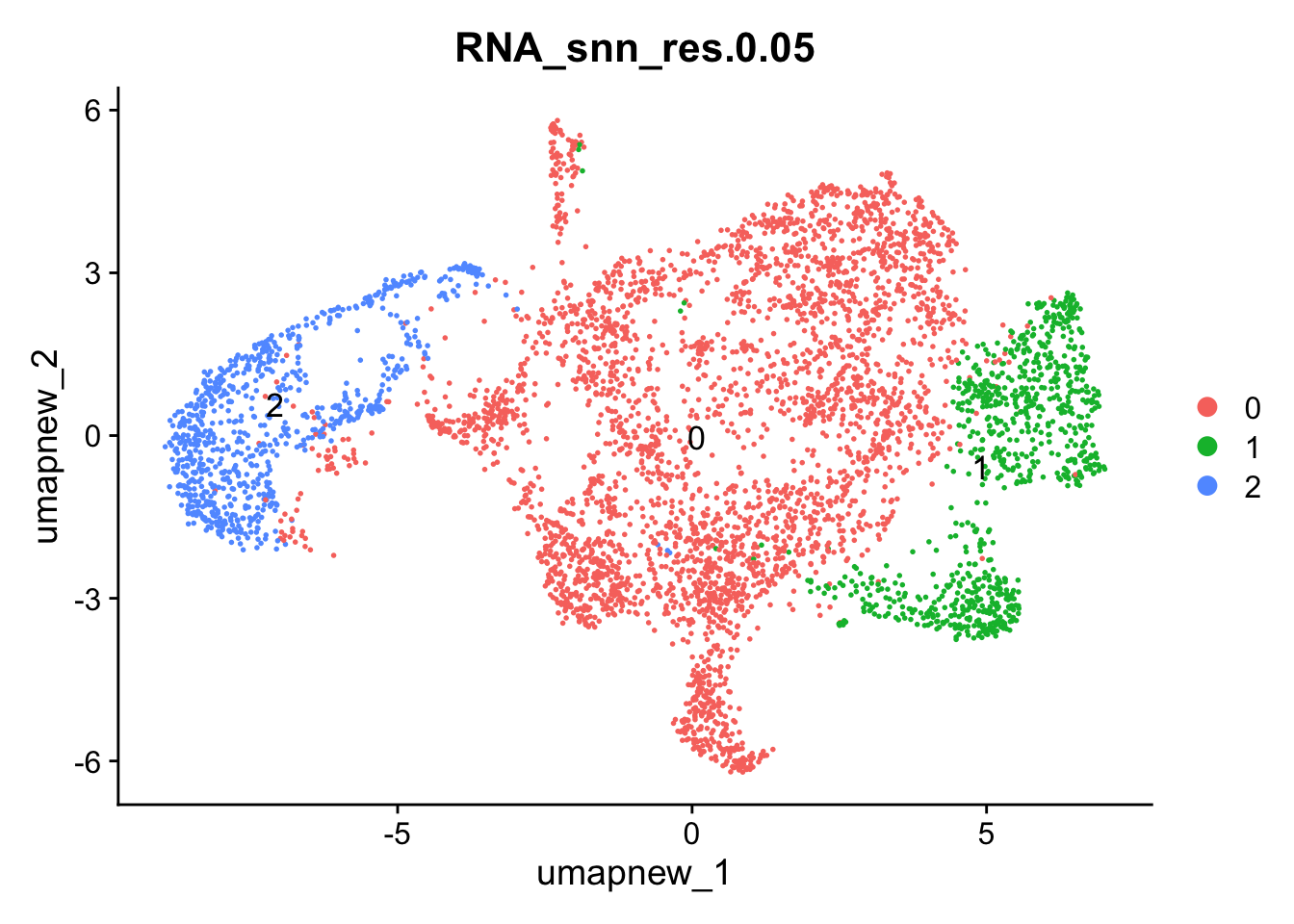
Selecting resolution as “0.05” to explore the top marker genes
opt_res <- "RNA_snn_res.0.05"
n <- nlevels(paed_sub$RNA_snn_res.0.05)
paed_sub$RNA_snn_res.0.05 <- factor(paed_sub$RNA_snn_res.0.05, levels = seq(0,n-1))
paed_sub$seurat_clusters <- NULL
Idents(paed_sub) <- paed_sub$RNA_snn_res.0.05
paed_sub.markers <- FindAllMarkers(paed_sub, only.pos = TRUE, min.pct = 0.25, logfc.threshold = 0.25)Calculating cluster 0Calculating cluster 1Calculating cluster 2paed_sub.markers %>%
group_by(cluster) %>% unique() %>%
top_n(n = 5, wt = avg_log2FC) -> top5
paed_sub.markers %>%
group_by(cluster) %>%
slice_head(n=1) %>%
pull(gene) -> best.wilcox.gene.per.cluster
best.wilcox.gene.per.cluster[1] "GSTP1" "DUOXA2" "PTGFR" FeaturePlot(paed_sub,features=best.wilcox.gene.per.cluster, reduction = 'umap.new', raster = FALSE, label = T, ncol = 2)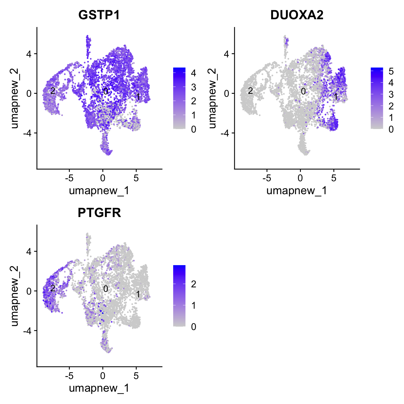
| Version | Author | Date |
|---|---|---|
| a94371e | Gunjan Dixit | 2024-06-07 |
out_markers <- here("output",
            "CSV",
            paste(tissue,"_Marker_genes_Reclustered_Basal_population.",opt_res, sep = ""))

dir.create(out_markers, recursive = TRUE, showWarnings = FALSE)

for (cl in unique(paed_sub.markers$cluster)) {
  cluster_data <- paed_sub.markers %>% dplyr::filter(cluster == cl)
  file_name <- here(out_markers, paste0("G000231_Neeland_",tissue, "_cluster_", cl, ".csv"))
  write.csv(cluster_data, file = file_name)
}
Expression of known marker genes
Goblet cells (Bronchial, Nasal and subsegmental)
LYPD2 and PSCA are specific to Nasal. BPIFB1, C16orf89 and NPDC1 are specific to subsegmental.
known_markers <- c("FXYD3","EPCAM", "ELF3", "IGFBP2", "SERPINF1", "TSPAN1", "GPX8", "ALDH1A3", "CEACAM5", "LYPD2", "PSCA", "BPIFB1", "C16orf89", "NPDC1")
FeaturePlot(paed_sub,features=known_markers, reduction = 'umap.new', raster = FALSE, label = T, ncol = 3)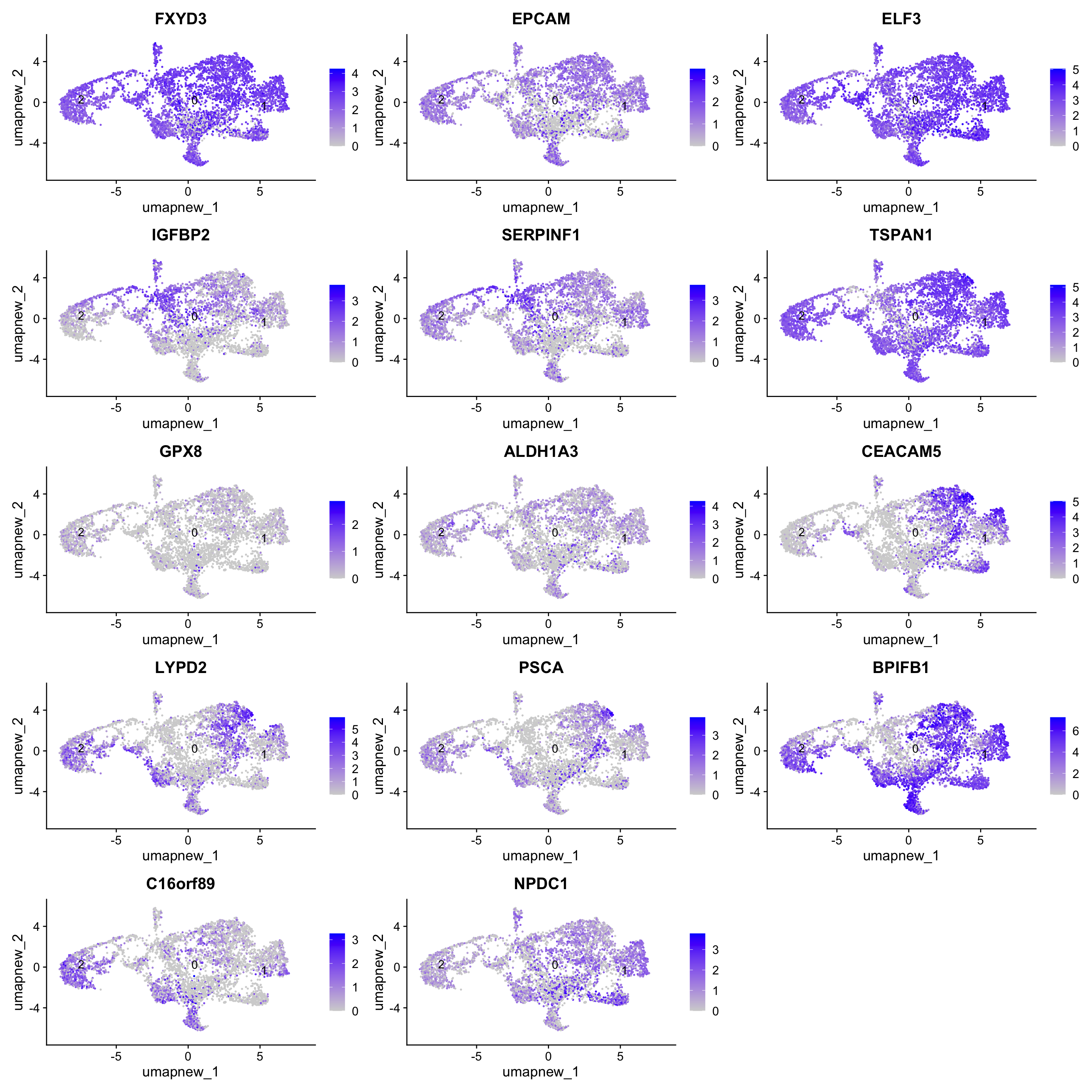
| Version | Author | Date |
|---|---|---|
| a94371e | Gunjan Dixit | 2024-06-07 |
Club cells
club_markers <- c("SERPINB3", "TCN1", "ASRGL1")
FeaturePlot(paed_sub,features=club_markers, reduction = 'umap.new', raster = FALSE, label = T, ncol = 2)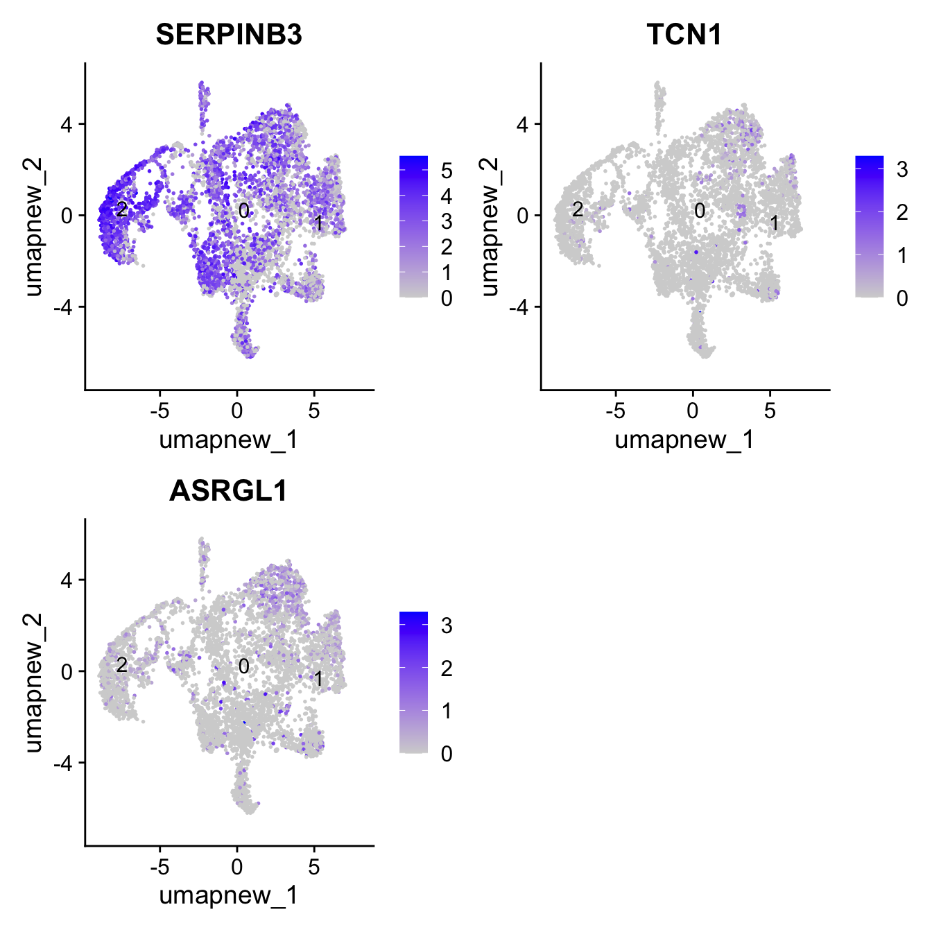
| Version | Author | Date |
|---|---|---|
| a94371e | Gunjan Dixit | 2024-06-07 |
Basal cells
Note: These markers are only specific to Basal
basal_markers <- c("KRT15", "KRT17", "TP63")
FeaturePlot(paed_sub,features=basal_markers, reduction = 'umap.new', raster = FALSE, label = T, ncol = 2)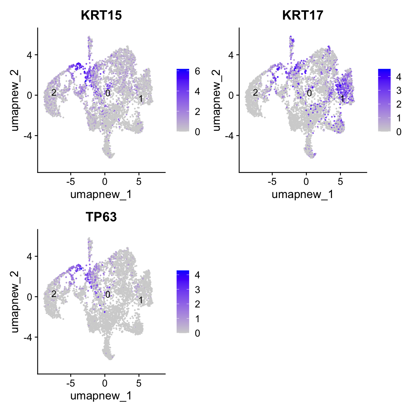
| Version | Author | Date |
|---|---|---|
| a94371e | Gunjan Dixit | 2024-06-07 |
Azimuth Labels
## Finest level
DimPlot(paed_sub, reduction = "umap.new", group.by = "predicted.ann_finest_level", raster = FALSE, repel = TRUE, label = TRUE, label.size = 3.5) 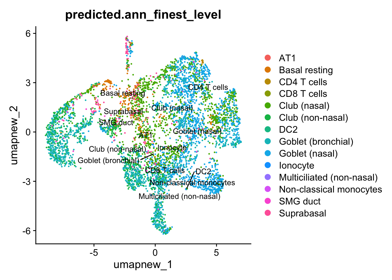
| Version | Author | Date |
|---|---|---|
| a94371e | Gunjan Dixit | 2024-06-07 |
df_table <- as.data.frame(table(paed_sub$RNA_snn_res.0.05, paed_sub$predicted.ann_finest_level))
ggplot(df_table, aes(Var1, Freq, fill = Var2)) +
  geom_bar(stat = "identity") +
  labs(x = "RNA_snn_res.0.05", y = "Count", fill = "predicted ann_finest_level") +
  theme_minimal() +
  ggtitle("Stacked Bar Plot of basal/club/goblet (res=0.05) and predicted.ann_finest_level")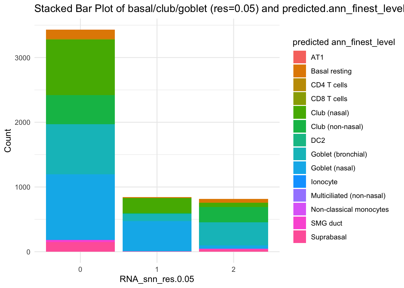
| Version | Author | Date |
|---|---|---|
| a94371e | Gunjan Dixit | 2024-06-07 |
## Predicted_Level 5
DimPlot(paed_sub, reduction = "umap.new", group.by = "predicted.ann_level_5", raster = FALSE, repel = TRUE, label = TRUE, label.size = 3.5) 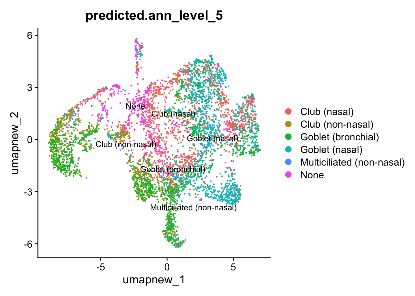
| Version | Author | Date |
|---|---|---|
| a94371e | Gunjan Dixit | 2024-06-07 |
df_table <- as.data.frame(table(paed_sub$RNA_snn_res.0.05, paed_sub$predicted.ann_level_5))

ggplot(df_table, aes(Var1, Freq, fill = Var2)) +
  geom_bar(stat = "identity") +
  labs(x = "RNA_snn_res.0.05", y = "Count", fill = "predicted ann_level_5") +
  theme_minimal() +
  ggtitle("Stacked Bar Plot of basal/club/goblet (res=0.05) and predicted.ann_level5")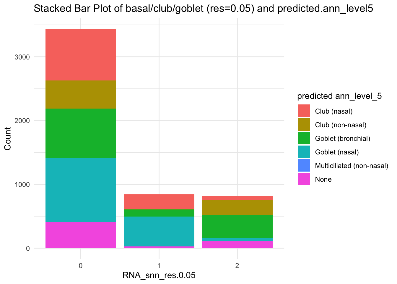
| Version | Author | Date |
|---|---|---|
| a94371e | Gunjan Dixit | 2024-06-07 |
Exploring clusters at resolution 0.1 to 1
paed_sub <- paed_sub %>%
  NormalizeData() %>%
  FindVariableFeatures() %>%
  ScaleData() %>%
  RunPCA()

paed_sub <- RunUMAP(paed_sub, dims = 1:30, reduction = "pca", reduction.name = "umap.new")

meta_data <- colnames(paed_sub@meta.data)
drop <- grep("^RNA_snn_res", meta_data, value = TRUE)
paed_sub@meta.data <- paed_sub@meta.data[, !(colnames(paed_sub@meta.data) %in% drop)]


resolutions <- seq(0.1, 1, by = 0.1)
paed_sub <- FindNeighbors(paed_sub, reduction = "pca", dims = 1:30)
paed_sub <- FindClusters(paed_sub, resolution = resolutions, algorithm = 3)
Modularity Optimizer version 1.3.0 by Ludo Waltman and Nees Jan van Eck
Number of nodes: 5091
Number of edges: 186471
Running smart local moving algorithm...
Maximum modularity in 10 random starts: 0.9374
Number of communities: 5
Elapsed time: 1 seconds
Modularity Optimizer version 1.3.0 by Ludo Waltman and Nees Jan van Eck
Number of nodes: 5091
Number of edges: 186471
Running smart local moving algorithm...
Maximum modularity in 10 random starts: 0.9177
Number of communities: 8
Elapsed time: 1 seconds
Modularity Optimizer version 1.3.0 by Ludo Waltman and Nees Jan van Eck
Number of nodes: 5091
Number of edges: 186471
Running smart local moving algorithm...
Maximum modularity in 10 random starts: 0.9020
Number of communities: 9
Elapsed time: 1 seconds
Modularity Optimizer version 1.3.0 by Ludo Waltman and Nees Jan van Eck
Number of nodes: 5091
Number of edges: 186471
Running smart local moving algorithm...
Maximum modularity in 10 random starts: 0.8887
Number of communities: 12
Elapsed time: 1 seconds
Modularity Optimizer version 1.3.0 by Ludo Waltman and Nees Jan van Eck
Number of nodes: 5091
Number of edges: 186471
Running smart local moving algorithm...
Maximum modularity in 10 random starts: 0.8767
Number of communities: 13
Elapsed time: 1 seconds
Modularity Optimizer version 1.3.0 by Ludo Waltman and Nees Jan van Eck
Number of nodes: 5091
Number of edges: 186471
Running smart local moving algorithm...
Maximum modularity in 10 random starts: 0.8670
Number of communities: 14
Elapsed time: 1 seconds
Modularity Optimizer version 1.3.0 by Ludo Waltman and Nees Jan van Eck
Number of nodes: 5091
Number of edges: 186471
Running smart local moving algorithm...
Maximum modularity in 10 random starts: 0.8574
Number of communities: 14
Elapsed time: 1 seconds
Modularity Optimizer version 1.3.0 by Ludo Waltman and Nees Jan van Eck
Number of nodes: 5091
Number of edges: 186471
Running smart local moving algorithm...
Maximum modularity in 10 random starts: 0.8481
Number of communities: 15
Elapsed time: 1 seconds
Modularity Optimizer version 1.3.0 by Ludo Waltman and Nees Jan van Eck
Number of nodes: 5091
Number of edges: 186471
Running smart local moving algorithm...
Maximum modularity in 10 random starts: 0.8398
Number of communities: 16
Elapsed time: 1 seconds
Modularity Optimizer version 1.3.0 by Ludo Waltman and Nees Jan van Eck
Number of nodes: 5091
Number of edges: 186471
Running smart local moving algorithm...
Maximum modularity in 10 random starts: 0.8318
Number of communities: 17
Elapsed time: 1 secondsDimHeatmap(paed_sub, dims = 1:10, cells = 500, balanced = TRUE)
| Version | Author | Date |
|---|---|---|
| a94371e | Gunjan Dixit | 2024-06-07 |
clustree(paed_sub, prefix = "RNA_snn_res.")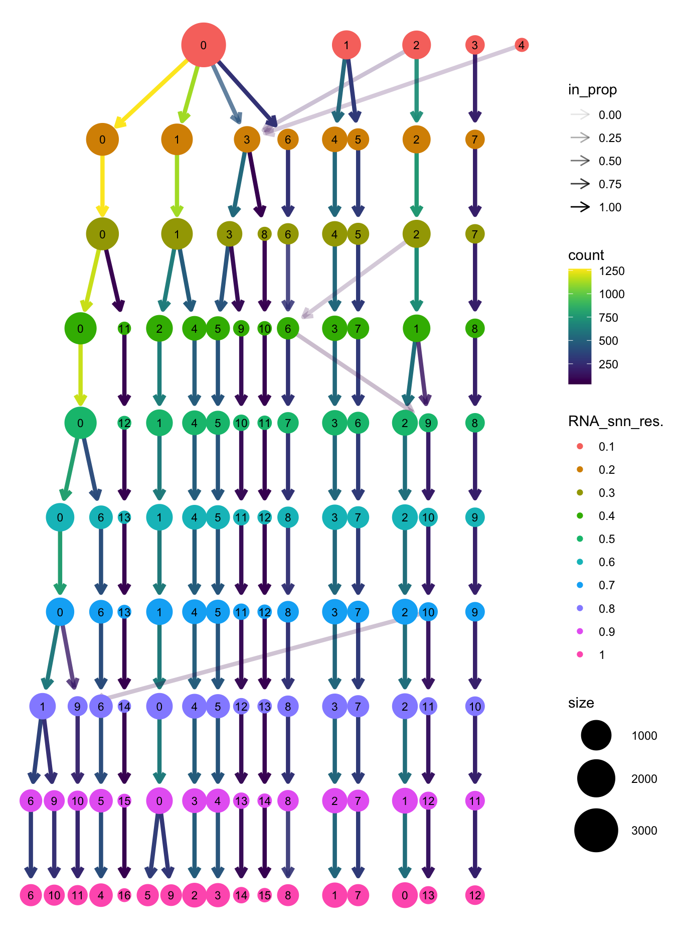
| Version | Author | Date |
|---|---|---|
| a94371e | Gunjan Dixit | 2024-06-07 |
DimPlot(paed_sub, reduction = "umap.new", group.by = "RNA_snn_res.0.1" , label = TRUE, label.size = 4.5, repel = TRUE, raster = FALSE )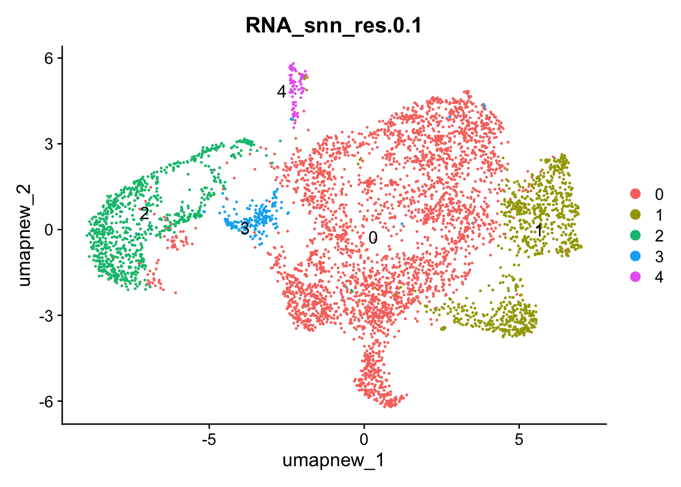
| Version | Author | Date |
|---|---|---|
| a94371e | Gunjan Dixit | 2024-06-07 |
Selecting resolution as “0.1” to explore the top marker genes
opt_res <- "RNA_snn_res.0.1"
n <- nlevels(paed_sub$RNA_snn_res.0.1)
paed_sub$RNA_snn_res.0.1 <- factor(paed_sub$RNA_snn_res.0.1, levels = seq(0,n-1))
paed_sub$seurat_clusters <- NULL
Idents(paed_sub) <- paed_sub$RNA_snn_res.0.1
paed_sub.markers <- FindAllMarkers(paed_sub, only.pos = TRUE, min.pct = 0.25, logfc.threshold = 0.25)Calculating cluster 0Calculating cluster 1Calculating cluster 2Calculating cluster 3Calculating cluster 4paed_sub.markers %>%
group_by(cluster) %>% unique() %>%
top_n(n = 5, wt = avg_log2FC) -> top5
paed_sub.markers %>%
group_by(cluster) %>%
slice_head(n=1) %>%
pull(gene) -> best.wilcox.gene.per.cluster
best.wilcox.gene.per.cluster[1] "CD74" "DUOXA2" "PTGFR" "FOSB" "ASF1B" FeaturePlot(paed_sub,features=best.wilcox.gene.per.cluster, reduction = 'umap.new', raster = FALSE, label = T, ncol = 2)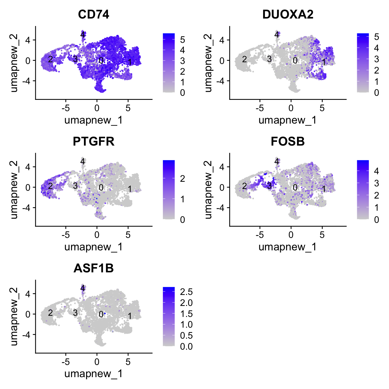
| Version | Author | Date |
|---|---|---|
| a94371e | Gunjan Dixit | 2024-06-07 |
out_markers <- here("output",
            "CSV",
            paste(tissue,"_Marker_genes_Reclustered_Basal_population.",opt_res, sep = ""))

dir.create(out_markers, recursive = TRUE, showWarnings = FALSE)

for (cl in unique(paed_sub.markers$cluster)) {
  cluster_data <- paed_sub.markers %>% dplyr::filter(cluster == cl)
  file_name <- here(out_markers, paste0("G000231_Neeland_",tissue, "_cluster_", cl, ".csv"))
  write.csv(cluster_data, file = file_name)
}
Reclustering T cell population
This includes CD4 T cell, CD8 T cell, NK cell, NK-T cell, proliferating or cycling T/NK cell.
The marker genes for this reclustering can be found here-
idx <- which(Idents(seu_obj) %in% c("CD4 T cells", "CD8 T cells", "proliferating T/NK"))
paed_sub <- seu_obj[,idx]
mito_genes <- grep("^MT-", rownames(paed_sub), value = TRUE)
paed_sub <- subset(paed_sub, features = setdiff(rownames(paed_sub), mito_genes))
paed_sub
An object of class Seurat
18035 features across 7632 samples within 1 assay
Active assay: RNA (18035 features, 1995 variable features)
3 layers present: counts, data, scale.data
3 dimensional reductions calculated: pca, umap, umap.unintegratedpaed_sub <- paed_sub %>%
NormalizeData() %>%
FindVariableFeatures() %>%
ScaleData() %>%
RunPCA()
paed_sub <- RunUMAP(paed_sub, dims = 1:30, reduction = "pca", reduction.name = "umap.new")
meta_data <- colnames(paed_sub@meta.data)
drop <- grep("^RNA_snn_res", meta_data, value = TRUE)
paed_sub@meta.data <- paed_sub@meta.data[, !(colnames(paed_sub@meta.data) %in% drop)]
resolutions <- seq(0.1, 1, by = 0.1)
paed_sub <- FindNeighbors(paed_sub, reduction = "pca", dims = 1:30)
paed_sub <- FindClusters(paed_sub, resolution = resolutions, algorithm = 3)Modularity Optimizer version 1.3.0 by Ludo Waltman and Nees Jan van Eck
Number of nodes: 7632
Number of edges: 279916
Running smart local moving algorithm...
Maximum modularity in 10 random starts: 0.9447
Number of communities: 7
Elapsed time: 4 seconds
Modularity Optimizer version 1.3.0 by Ludo Waltman and Nees Jan van Eck
Number of nodes: 7632
Number of edges: 279916
Running smart local moving algorithm...
Maximum modularity in 10 random starts: 0.9200
Number of communities: 9
Elapsed time: 3 seconds
Modularity Optimizer version 1.3.0 by Ludo Waltman and Nees Jan van Eck
Number of nodes: 7632
Number of edges: 279916
Running smart local moving algorithm...
Maximum modularity in 10 random starts: 0.9041
Number of communities: 10
Elapsed time: 3 seconds
Modularity Optimizer version 1.3.0 by Ludo Waltman and Nees Jan van Eck
Number of nodes: 7632
Number of edges: 279916
Running smart local moving algorithm...
Maximum modularity in 10 random starts: 0.8890
Number of communities: 11
Elapsed time: 3 seconds
Modularity Optimizer version 1.3.0 by Ludo Waltman and Nees Jan van Eck
Number of nodes: 7632
Number of edges: 279916
Running smart local moving algorithm...
Maximum modularity in 10 random starts: 0.8743
Number of communities: 12
Elapsed time: 3 seconds
Modularity Optimizer version 1.3.0 by Ludo Waltman and Nees Jan van Eck
Number of nodes: 7632
Number of edges: 279916
Running smart local moving algorithm...
Maximum modularity in 10 random starts: 0.8605
Number of communities: 13
Elapsed time: 3 seconds
Modularity Optimizer version 1.3.0 by Ludo Waltman and Nees Jan van Eck
Number of nodes: 7632
Number of edges: 279916
Running smart local moving algorithm...
Maximum modularity in 10 random starts: 0.8484
Number of communities: 15
Elapsed time: 2 seconds
Modularity Optimizer version 1.3.0 by Ludo Waltman and Nees Jan van Eck
Number of nodes: 7632
Number of edges: 279916
Running smart local moving algorithm...
Maximum modularity in 10 random starts: 0.8392
Number of communities: 18
Elapsed time: 2 seconds
Modularity Optimizer version 1.3.0 by Ludo Waltman and Nees Jan van Eck
Number of nodes: 7632
Number of edges: 279916
Running smart local moving algorithm...
Maximum modularity in 10 random starts: 0.8308
Number of communities: 20
Elapsed time: 2 seconds
Modularity Optimizer version 1.3.0 by Ludo Waltman and Nees Jan van Eck
Number of nodes: 7632
Number of edges: 279916
Running smart local moving algorithm...
Maximum modularity in 10 random starts: 0.8230
Number of communities: 21
Elapsed time: 2 secondsDimHeatmap(paed_sub, dims = 1:10, cells = 500, balanced = TRUE)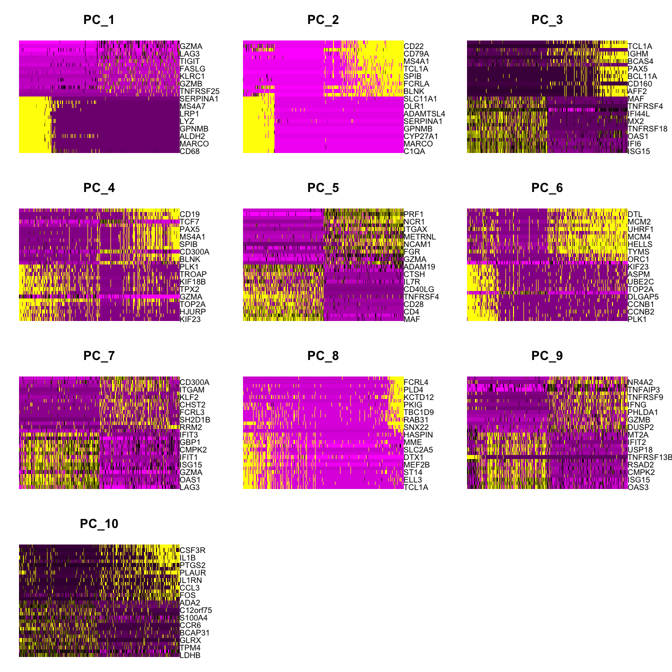
clustree(paed_sub, prefix = "RNA_snn_res.")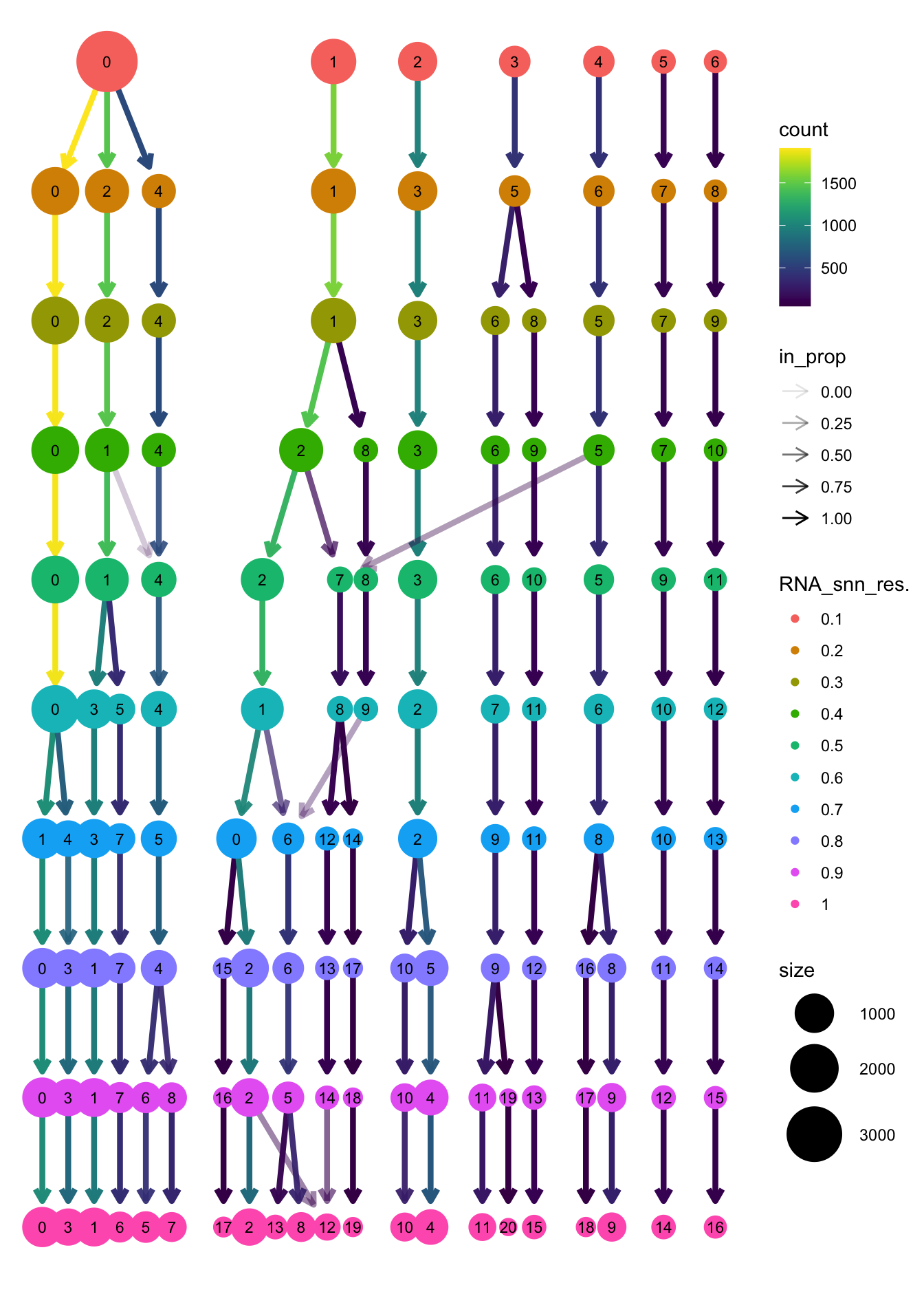
opt_res <- "RNA_snn_res.0.4"
n <- nlevels(paed_sub$RNA_snn_res.0.4)
paed_sub$RNA_snn_res.0.4 <- factor(paed_sub$RNA_snn_res.0.4, levels = seq(0,n-1))
paed_sub$seurat_clusters <- NULL
paed_sub$cluster <- paed_sub$RNA_snn_res.0.4
Idents(paed_sub) <- paed_sub$cluster
paed_sub.markers <- FindAllMarkers(paed_sub, only.pos = TRUE, min.pct = 0.25, logfc.threshold = 0.25)Calculating cluster 0Calculating cluster 1Calculating cluster 2Calculating cluster 3Calculating cluster 4Calculating cluster 5Calculating cluster 6Calculating cluster 7Calculating cluster 8Calculating cluster 9Calculating cluster 10paed_sub.markers %>%
group_by(cluster) %>% unique() %>%
top_n(n = 5, wt = avg_log2FC) -> top5
paed_sub.markers %>%
group_by(cluster) %>%
slice_head(n=1) %>%
pull(gene) -> best.wilcox.gene.per.cluster
best.wilcox.gene.per.cluster [1] "CD8A" "HOPX" "MAF" "TCF7" "LAG3" "TYROBP" "UHRF1"
[8] "CSF3R" "NOG" "POU2AF1" "GPNMB" Feature plot shows the expression of top marker genes per cluster.
FeaturePlot(paed_sub,features=best.wilcox.gene.per.cluster, reduction = 'umap.new', raster = FALSE, ncol = 2, label = TRUE)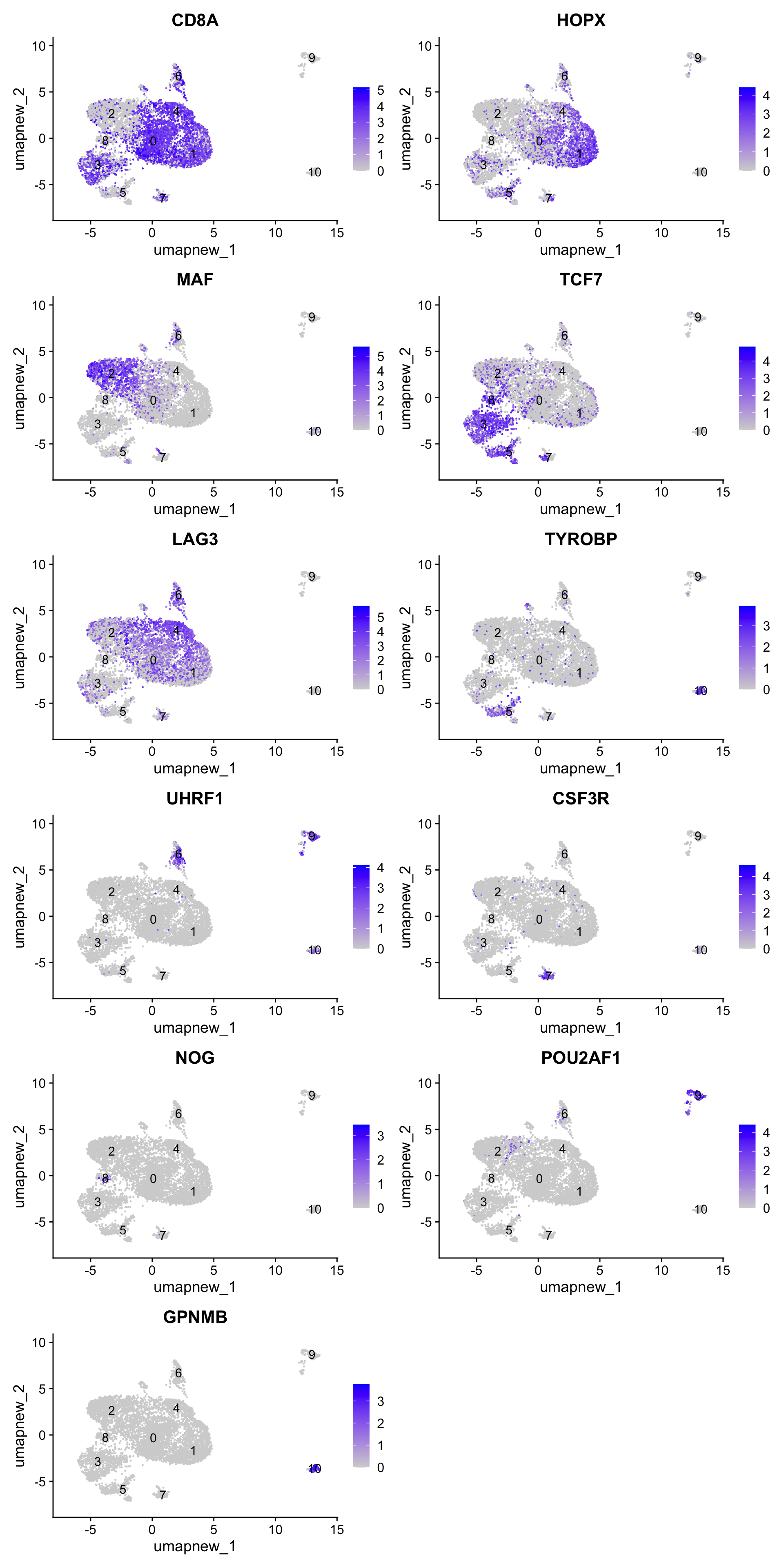
Top 10 marker genes from Seurat
## Seurat top markers
top10 <- paed_sub.markers %>%
    group_by(cluster) %>%
    top_n(n = 10, wt = avg_log2FC) %>%
    ungroup() %>%
    distinct(gene, .keep_all = TRUE) %>%
    arrange(cluster, desc(avg_log2FC))

cluster_colors <- paletteer::paletteer_d("pals::glasbey")[factor(top10$cluster)]

DotPlot(paed_sub,
        features = unique(top10$gene),
        group.by = opt_res,
        cols = c("azure1", "blueviolet"),
        dot.scale = 3, assay = "RNA") +
    RotatedAxis() +
    FontSize(y.text = 8, x.text = 12) +
    labs(y = element_blank(), x = element_blank()) +
    coord_flip() +
    theme(axis.text.y = element_text(color = cluster_colors)) +
    ggtitle("Top 10 marker genes per cluster (Seurat)")
Warning: Vectorized input to `element_text()` is not officially supported.
ℹ Results may be unexpected or may change in future versions of ggplot2.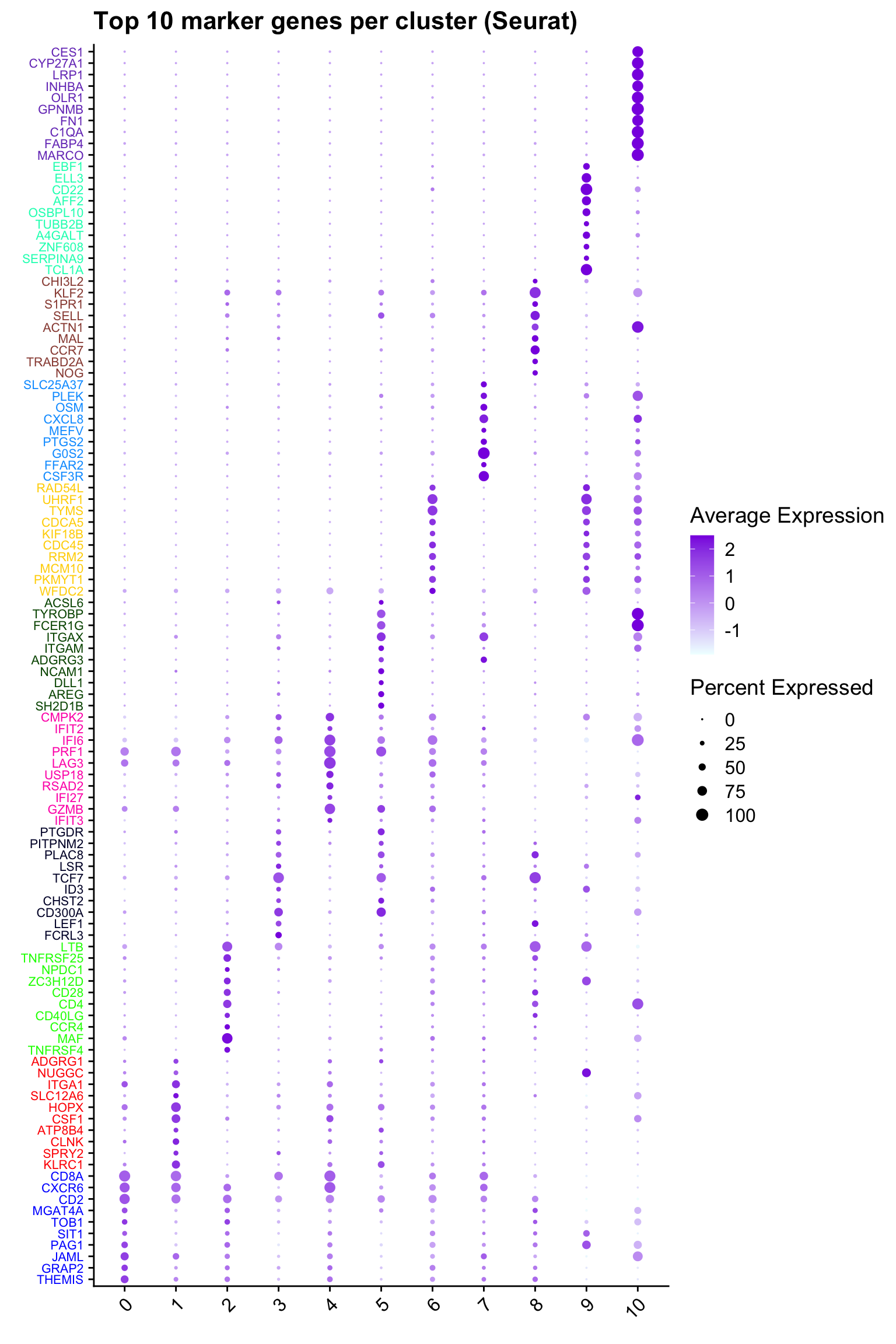
| Version | Author | Date |
|---|---|---|
| c20f60f | Gunjan Dixit | 2024-07-08 |
out_markers <- here("output",
            "CSV",
            paste(tissue,"_Marker_genes_Reclustered_Tcell_population.",opt_res, sep = ""))

dir.create(out_markers, recursive = TRUE, showWarnings = FALSE)

for (cl in unique(paed_sub.markers$cluster)) {
  cluster_data <- paed_sub.markers %>% dplyr::filter(cluster == cl)
  file_name <- here(out_markers, paste0("G000231_Neeland_",tissue, "_cluster_", cl, ".csv"))
  write.csv(cluster_data, file = file_name)
}
Update T cell subclustering labels
cell_labels <- readxl::read_excel(here("data/Cell_labels_Mel_v2/earlyAIR_NB_BB_BAL_T-NK_annotations_16.07.24.xlsx"), sheet = "BB")
new_cluster_names <- cell_labels %>%
  dplyr::select(cluster, annotation) %>%
  deframe()

paed_sub <- RenameIdents(paed_sub, new_cluster_names)
paed_sub@meta.data$cell_labels_v2 <- Idents(paed_sub)

DimPlot(paed_sub, reduction = "umap.new", raster = FALSE, repel = TRUE, label = TRUE, label.size = 3.5) + ggtitle(paste0(tissue, ": UMAP with Updated subclustering"))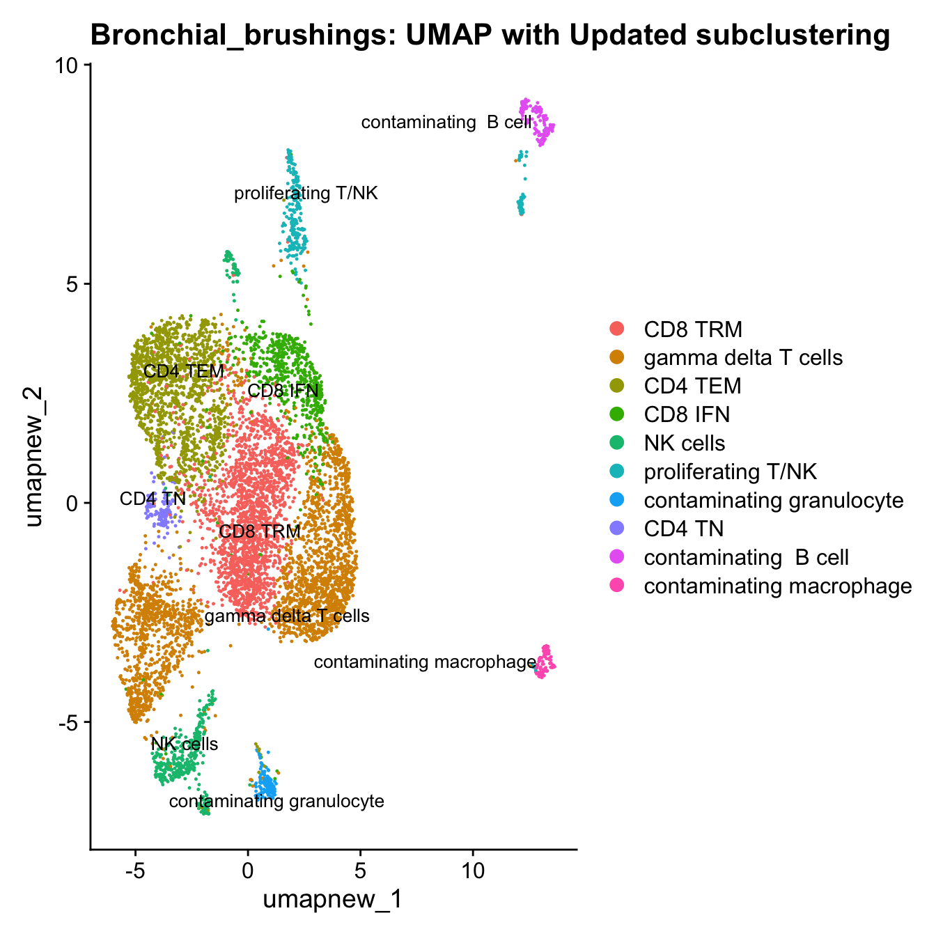
Excluding contaminating labels
idx <- which(grepl("^contaminating", Idents(paed_sub)))
paed_clean <- paed_sub[, -idx]
DimPlot(paed_clean, reduction = "umap.new", raster = FALSE, repel = TRUE, label = TRUE, label.size = 3.5) + ggtitle(paste0(tissue, ": Updated subclustering (clean)"))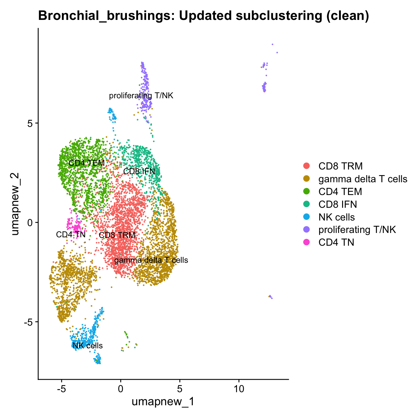
paed_clean <- paed_clean %>%
NormalizeData() %>%
FindVariableFeatures() %>%
ScaleData() %>%
RunPCA()
Normalizing layer: countsFinding variable features for layer countsCentering and scaling data matrixWarning: Different features in new layer data than already exists for
scale.dataPC_ 1
Positive: JAML, FCRL6, NMUR1, IL7R, TRGC2, ITGA1, CLNK, KLRD1, HOPX, MATK
TRGC1, KLRC3, PTGDR, KLRC1, OBSCN, TNFAIP3, CCL4, TNFSF14, THEMIS, KLRB1
CSF1, CXCR4, ST8SIA1, ITGAD, TRBC1, PTGER4, LINC02694, SPRY1, NELL2, CTSW
Negative: MYBL2, TYMS, KIFC1, UHRF1, AURKB, ZWINT, MKI67, RRM2, PKMYT1, TK1
CDT1, HIST1H1B, FOXM1, CDCA5, TOP2A, BIRC5, ASF1B, E2F2, ESPL1, CDC45
PCLAF, E2F1, KIF2C, GTSE1, CDCA8, RAD54L, HIST1H2BH, SPC24, SHCBP1, STMN1
PC_ 2
Positive: HOPX, ITGA1, NMUR1, SCUBE1, CLNK, JAML, CAPG, KLRC1, FCRL6, GZMA
CSF1, CCL4, CD160, TRGC2, ADGRG1, KLRD1, KLRC3, PELO, IGHM, SLAMF8
HIST1H1C, AMZ1, CRIM1, AURKB, ITGAD, ITM2C, ADGRG5, ENTPD1, KIFC1, SPRY2
Negative: ISG15, OAS3, IFI6, IRF7, MX1, IFI44L, OAS1, MX2, CMPK2, FURIN
ISG20, IFIT1, IFI44, RSAD2, SOCS3, TNFRSF18, BCL3, HAPLN3, SAT1, HELZ2
OAS2, XAF1, IFI35, USP18, SATB1, LY6E, STAT2, CREM, IFIT3, HERC6
PC_ 3
Positive: MAF, CD4, LTB, CD28, TNFRSF25, ZC3H12D, TNFRSF4, CCR4, CD5, CD40LG
CCR6, CTSH, ICOS, SLAMF1, ADAM19, IL7R, RORA, FLT3LG, CTLA4, BCL2
PIM2, COL5A3, ERN1, AQP3, GPR183, NPDC1, S100A4, IL4I1, CD82, CCR2
Negative: NKG7, GNLY, CTSW, PRF1, KLRD1, PIK3AP1, GZMB, KLRC3, NCR1, ITGAX
HOPX, MATK, METRNL, CD300A, KIR2DL4, KLRC1, IFI6, BST2, FGR, MX1
CMPK2, TRDC, IFITM3, PLCG2, IFI44L, FCRL6, RSAD2, NCAM1, GFOD1, TYROBP
PC_ 4
Positive: SPIB, TNFRSF13B, WDFY4, SYK, PAX5, CD19, MS4A1, CD22, KCTD12, BASP1
BANK1, FCRL5, MPEG1, CD79A, CYBB, DOK3, PLD4, BLNK, IGHA1, SNX22
BHLHE41, FCRL4, SPI1, PKIG, SWAP70, CBFA2T3, TBC1D9, HCK, TSPAN33, FCRLA
Negative: GZMA, LAG3, CCR5, MKI67, RRM2, S100A4, HJURP, BIRC5, GZMB, FASLG
SPC24, CENPF, THEMIS, ASPM, STMN1, ANXA5, PRF1, GTSE1, CCL4, GPR25
NUSAP1, CXCL13, CSF1, GZMH, TK1, CCNA2, HIST1H1B, SCUBE1, CCNB2, TPX2
PC_ 5
Positive: LAG3, GZMA, CCR5, FASLG, CSF1, CCL4, PTMS, JAML, GZMB, ENTPD1
MX1, PRDM1, TYMP, PRF1, GPR25, GBP5, ADAM19, USP18, GBP1, OAS1
ZBP1, ZEB2, CD74, SAMD9L, THEMIS, RSAD2, TNFRSF13B, RORA, SPIB, CYBB
Negative: TCF7, CD300A, LEF1, KLF2, ITGAM, PLAC8, ITGAX, GAS7, PTGDR, TIAM1
FCRL3, DTX1, CHST2, FCER1G, TXK, TYROBP, AREG, TNFRSF18, SELL, SH2D1B
LTBP3, ACSL6, CD27, FGR, BACH2, TRDC, PITPNM2, ACTN1, SORL1, FOS paed_clean <- RunUMAP(paed_clean, dims = 1:30, reduction = "pca", reduction.name = "umap.clean")12:15:11 UMAP embedding parameters a = 0.9922 b = 1.112Found more than one class "dist" in cache; using the first, from namespace 'spam'Also defined by 'BiocGenerics'12:15:11 Read 7267 rows and found 30 numeric columns12:15:11 Using Annoy for neighbor search, n_neighbors = 30Found more than one class "dist" in cache; using the first, from namespace 'spam'Also defined by 'BiocGenerics'12:15:11 Building Annoy index with metric = cosine, n_trees = 500% 10 20 30 40 50 60 70 80 90 100%[----|----|----|----|----|----|----|----|----|----|**************************************************|
12:15:11 Writing NN index file to temp file /var/folders/q8/kw1r78g12qn793xm7g0zvk94x2bh70/T//RtmpjdQJLp/file139036b7e675
12:15:11 Searching Annoy index using 1 thread, search_k = 3000
12:15:12 Annoy recall = 100%
12:15:13 Commencing smooth kNN distance calibration using 1 thread with target n_neighbors = 30
12:15:13 Initializing from normalized Laplacian + noise (using RSpectra)
12:15:13 Commencing optimization for 500 epochs, with 305604 positive edges
12:15:19 Optimization finishedDimPlot(paed_clean, reduction = "umap.clean", group.by = "cell_labels_v2",raster = FALSE, repel = TRUE, label = TRUE, label.size = 4.5) + ggtitle(paste0(tissue, ": Updated subclustering (clean)"))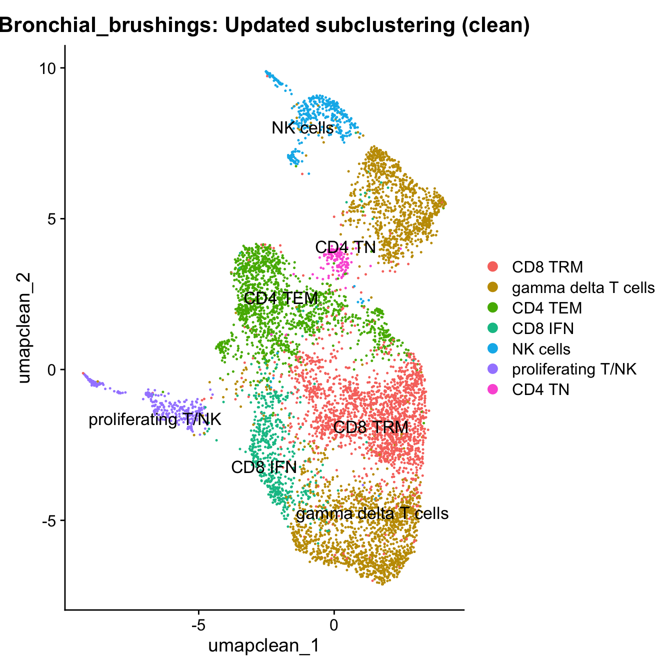
Session Info
sessioninfo::session_info()─ Session info ───────────────────────────────────────────────────────────────
setting value
version R version 4.3.2 (2023-10-31)
os macOS Sonoma 14.5
system aarch64, darwin20
ui X11
language (EN)
collate en_US.UTF-8
ctype en_US.UTF-8
tz Australia/Melbourne
date 2024-07-26
pandoc 3.1.1 @ /Users/dixitgunjan/Desktop/RStudio.app/Contents/Resources/app/quarto/bin/tools/ (via rmarkdown)
─ Packages ───────────────────────────────────────────────────────────────────
package * version date (UTC) lib source
abind 1.4-5 2016-07-21 [1] CRAN (R 4.3.0)
AnnotationDbi * 1.64.1 2023-11-02 [1] Bioconductor
backports 1.4.1 2021-12-13 [1] CRAN (R 4.3.0)
beeswarm 0.4.0 2021-06-01 [1] CRAN (R 4.3.0)
Biobase * 2.62.0 2023-10-26 [1] Bioconductor
BiocGenerics * 0.48.1 2023-11-02 [1] Bioconductor
BiocManager 1.30.22 2023-08-08 [1] CRAN (R 4.3.0)
BiocStyle * 2.30.0 2023-10-26 [1] Bioconductor
Biostrings 2.70.2 2024-01-30 [1] Bioconductor 3.18 (R 4.3.2)
bit 4.0.5 2022-11-15 [1] CRAN (R 4.3.0)
bit64 4.0.5 2020-08-30 [1] CRAN (R 4.3.0)
bitops 1.0-7 2021-04-24 [1] CRAN (R 4.3.0)
blob 1.2.4 2023-03-17 [1] CRAN (R 4.3.0)
bslib 0.6.1 2023-11-28 [1] CRAN (R 4.3.1)
cachem 1.0.8 2023-05-01 [1] CRAN (R 4.3.0)
callr 3.7.5 2024-02-19 [1] CRAN (R 4.3.1)
cellranger 1.1.0 2016-07-27 [1] CRAN (R 4.3.0)
checkmate 2.3.1 2023-12-04 [1] CRAN (R 4.3.1)
cli 3.6.2 2023-12-11 [1] CRAN (R 4.3.1)
cluster 2.1.6 2023-12-01 [1] CRAN (R 4.3.1)
clustree * 0.5.1 2023-11-05 [1] CRAN (R 4.3.1)
codetools 0.2-19 2023-02-01 [1] CRAN (R 4.3.2)
colorspace 2.1-0 2023-01-23 [1] CRAN (R 4.3.0)
cowplot 1.1.3 2024-01-22 [1] CRAN (R 4.3.1)
crayon 1.5.2 2022-09-29 [1] CRAN (R 4.3.0)
data.table * 1.15.0 2024-01-30 [1] CRAN (R 4.3.1)
DBI 1.2.2 2024-02-16 [1] CRAN (R 4.3.1)
DelayedArray 0.28.0 2023-11-06 [1] Bioconductor
deldir 2.0-2 2023-11-23 [1] CRAN (R 4.3.1)
digest 0.6.34 2024-01-11 [1] CRAN (R 4.3.1)
dotCall64 1.1-1 2023-11-28 [1] CRAN (R 4.3.1)
dplyr * 1.1.4 2023-11-17 [1] CRAN (R 4.3.1)
edgeR * 4.0.16 2024-02-20 [1] Bioconductor 3.18 (R 4.3.2)
ellipsis 0.3.2 2021-04-29 [1] CRAN (R 4.3.0)
evaluate 0.23 2023-11-01 [1] CRAN (R 4.3.1)
fansi 1.0.6 2023-12-08 [1] CRAN (R 4.3.1)
farver 2.1.1 2022-07-06 [1] CRAN (R 4.3.0)
fastDummies 1.7.3 2023-07-06 [1] CRAN (R 4.3.0)
fastmap 1.1.1 2023-02-24 [1] CRAN (R 4.3.0)
fitdistrplus 1.1-11 2023-04-25 [1] CRAN (R 4.3.0)
forcats * 1.0.0 2023-01-29 [1] CRAN (R 4.3.0)
fs 1.6.3 2023-07-20 [1] CRAN (R 4.3.0)
future 1.33.1 2023-12-22 [1] CRAN (R 4.3.1)
future.apply 1.11.1 2023-12-21 [1] CRAN (R 4.3.1)
generics 0.1.3 2022-07-05 [1] CRAN (R 4.3.0)
GenomeInfoDb 1.38.6 2024-02-10 [1] Bioconductor 3.18 (R 4.3.2)
GenomeInfoDbData 1.2.11 2024-02-27 [1] Bioconductor
GenomicRanges 1.54.1 2023-10-30 [1] Bioconductor
getPass 0.2-4 2023-12-10 [1] CRAN (R 4.3.1)
ggbeeswarm 0.7.2 2023-04-29 [1] CRAN (R 4.3.0)
ggforce 0.4.2 2024-02-19 [1] CRAN (R 4.3.1)
ggplot2 * 3.5.0 2024-02-23 [1] CRAN (R 4.3.1)
ggraph * 2.1.0 2022-10-09 [1] CRAN (R 4.3.0)
ggrastr 1.0.2 2023-06-01 [1] CRAN (R 4.3.0)
ggrepel 0.9.5 2024-01-10 [1] CRAN (R 4.3.1)
ggridges 0.5.6 2024-01-23 [1] CRAN (R 4.3.1)
git2r 0.33.0 2023-11-26 [1] CRAN (R 4.3.1)
globals 0.16.2 2022-11-21 [1] CRAN (R 4.3.0)
glue * 1.7.0 2024-01-09 [1] CRAN (R 4.3.1)
goftest 1.2-3 2021-10-07 [1] CRAN (R 4.3.0)
graphlayouts 1.1.0 2024-01-19 [1] CRAN (R 4.3.1)
gridExtra 2.3 2017-09-09 [1] CRAN (R 4.3.0)
gtable 0.3.4 2023-08-21 [1] CRAN (R 4.3.0)
here * 1.0.1 2020-12-13 [1] CRAN (R 4.3.0)
highr 0.10 2022-12-22 [1] CRAN (R 4.3.0)
hms 1.1.3 2023-03-21 [1] CRAN (R 4.3.0)
htmltools 0.5.7 2023-11-03 [1] CRAN (R 4.3.1)
htmlwidgets 1.6.4 2023-12-06 [1] CRAN (R 4.3.1)
httpuv 1.6.14 2024-01-26 [1] CRAN (R 4.3.1)
httr 1.4.7 2023-08-15 [1] CRAN (R 4.3.0)
ica 1.0-3 2022-07-08 [1] CRAN (R 4.3.0)
igraph 2.0.2 2024-02-17 [1] CRAN (R 4.3.1)
IRanges * 2.36.0 2023-10-26 [1] Bioconductor
irlba 2.3.5.1 2022-10-03 [1] CRAN (R 4.3.2)
jquerylib 0.1.4 2021-04-26 [1] CRAN (R 4.3.0)
jsonlite 1.8.8 2023-12-04 [1] CRAN (R 4.3.1)
kableExtra * 1.4.0 2024-01-24 [1] CRAN (R 4.3.1)
KEGGREST 1.42.0 2023-10-26 [1] Bioconductor
KernSmooth 2.23-22 2023-07-10 [1] CRAN (R 4.3.2)
knitr 1.45 2023-10-30 [1] CRAN (R 4.3.1)
labeling 0.4.3 2023-08-29 [1] CRAN (R 4.3.0)
later 1.3.2 2023-12-06 [1] CRAN (R 4.3.1)
lattice 0.22-5 2023-10-24 [1] CRAN (R 4.3.1)
lazyeval 0.2.2 2019-03-15 [1] CRAN (R 4.3.0)
leiden 0.4.3.1 2023-11-17 [1] CRAN (R 4.3.1)
lifecycle 1.0.4 2023-11-07 [1] CRAN (R 4.3.1)
limma * 3.58.1 2023-11-02 [1] Bioconductor
listenv 0.9.1 2024-01-29 [1] CRAN (R 4.3.1)
lmtest 0.9-40 2022-03-21 [1] CRAN (R 4.3.0)
locfit 1.5-9.8 2023-06-11 [1] CRAN (R 4.3.0)
lubridate * 1.9.3 2023-09-27 [1] CRAN (R 4.3.1)
magrittr 2.0.3 2022-03-30 [1] CRAN (R 4.3.0)
MASS 7.3-60.0.1 2024-01-13 [1] CRAN (R 4.3.1)
Matrix 1.6-5 2024-01-11 [1] CRAN (R 4.3.1)
MatrixGenerics 1.14.0 2023-10-26 [1] Bioconductor
matrixStats 1.2.0 2023-12-11 [1] CRAN (R 4.3.1)
memoise 2.0.1 2021-11-26 [1] CRAN (R 4.3.0)
mime 0.12 2021-09-28 [1] CRAN (R 4.3.0)
miniUI 0.1.1.1 2018-05-18 [1] CRAN (R 4.3.0)
munsell 0.5.0 2018-06-12 [1] CRAN (R 4.3.0)
nlme 3.1-164 2023-11-27 [1] CRAN (R 4.3.1)
org.Hs.eg.db * 3.18.0 2024-02-27 [1] Bioconductor
paletteer 1.6.0 2024-01-21 [1] CRAN (R 4.3.1)
parallelly 1.37.0 2024-02-14 [1] CRAN (R 4.3.1)
patchwork * 1.2.0 2024-01-08 [1] CRAN (R 4.3.1)
pbapply 1.7-2 2023-06-27 [1] CRAN (R 4.3.0)
pillar 1.9.0 2023-03-22 [1] CRAN (R 4.3.0)
pkgconfig 2.0.3 2019-09-22 [1] CRAN (R 4.3.0)
plotly 4.10.4 2024-01-13 [1] CRAN (R 4.3.1)
plyr 1.8.9 2023-10-02 [1] CRAN (R 4.3.1)
png 0.1-8 2022-11-29 [1] CRAN (R 4.3.0)
polyclip 1.10-6 2023-09-27 [1] CRAN (R 4.3.1)
presto 1.0.0 2024-02-27 [1] Github (immunogenomics/presto@31dc97f)
prismatic 1.1.1 2022-08-15 [1] CRAN (R 4.3.0)
processx 3.8.3 2023-12-10 [1] CRAN (R 4.3.1)
progressr 0.14.0 2023-08-10 [1] CRAN (R 4.3.0)
promises 1.2.1 2023-08-10 [1] CRAN (R 4.3.0)
ps 1.7.6 2024-01-18 [1] CRAN (R 4.3.1)
purrr * 1.0.2 2023-08-10 [1] CRAN (R 4.3.0)
R6 2.5.1 2021-08-19 [1] CRAN (R 4.3.0)
RANN 2.6.1 2019-01-08 [1] CRAN (R 4.3.0)
RColorBrewer * 1.1-3 2022-04-03 [1] CRAN (R 4.3.0)
Rcpp 1.0.12 2024-01-09 [1] CRAN (R 4.3.1)
RcppAnnoy 0.0.22 2024-01-23 [1] CRAN (R 4.3.1)
RcppHNSW 0.6.0 2024-02-04 [1] CRAN (R 4.3.1)
RCurl 1.98-1.14 2024-01-09 [1] CRAN (R 4.3.1)
readr * 2.1.5 2024-01-10 [1] CRAN (R 4.3.1)
readxl 1.4.3 2023-07-06 [1] CRAN (R 4.3.0)
rematch2 2.1.2 2020-05-01 [1] CRAN (R 4.3.0)
reshape2 1.4.4 2020-04-09 [1] CRAN (R 4.3.0)
reticulate 1.35.0 2024-01-31 [1] CRAN (R 4.3.1)
rlang 1.1.3 2024-01-10 [1] CRAN (R 4.3.1)
rmarkdown 2.25 2023-09-18 [1] CRAN (R 4.3.1)
ROCR 1.0-11 2020-05-02 [1] CRAN (R 4.3.0)
rprojroot 2.0.4 2023-11-05 [1] CRAN (R 4.3.1)
RSpectra 0.16-1 2022-04-24 [1] CRAN (R 4.3.0)
RSQLite 2.3.5 2024-01-21 [1] CRAN (R 4.3.1)
rstudioapi 0.15.0 2023-07-07 [1] CRAN (R 4.3.0)
Rtsne 0.17 2023-12-07 [1] CRAN (R 4.3.1)
S4Arrays 1.2.0 2023-10-26 [1] Bioconductor
S4Vectors * 0.40.2 2023-11-25 [1] Bioconductor 3.18 (R 4.3.2)
sass 0.4.8 2023-12-06 [1] CRAN (R 4.3.1)
scales 1.3.0 2023-11-28 [1] CRAN (R 4.3.1)
scattermore 1.2 2023-06-12 [1] CRAN (R 4.3.0)
sctransform 0.4.1 2023-10-19 [1] CRAN (R 4.3.1)
sessioninfo 1.2.2 2021-12-06 [1] CRAN (R 4.3.0)
Seurat * 5.0.1.9009 2024-02-28 [1] Github (satijalab/seurat@6a3ef5e)
SeuratObject * 5.0.1 2023-11-17 [1] CRAN (R 4.3.1)
shiny 1.8.0 2023-11-17 [1] CRAN (R 4.3.1)
SingleCellExperiment 1.24.0 2023-11-06 [1] Bioconductor
sp * 2.1-3 2024-01-30 [1] CRAN (R 4.3.1)
spam 2.10-0 2023-10-23 [1] CRAN (R 4.3.1)
SparseArray 1.2.4 2024-02-10 [1] Bioconductor 3.18 (R 4.3.2)
spatstat.data 3.0-4 2024-01-15 [1] CRAN (R 4.3.1)
spatstat.explore 3.2-6 2024-02-01 [1] CRAN (R 4.3.1)
spatstat.geom 3.2-8 2024-01-26 [1] CRAN (R 4.3.1)
spatstat.random 3.2-2 2023-11-29 [1] CRAN (R 4.3.1)
spatstat.sparse 3.0-3 2023-10-24 [1] CRAN (R 4.3.1)
spatstat.utils 3.0-4 2023-10-24 [1] CRAN (R 4.3.1)
speckle * 1.2.0 2023-10-26 [1] Bioconductor
statmod 1.5.0 2023-01-06 [1] CRAN (R 4.3.0)
stringi 1.8.3 2023-12-11 [1] CRAN (R 4.3.1)
stringr * 1.5.1 2023-11-14 [1] CRAN (R 4.3.1)
SummarizedExperiment 1.32.0 2023-11-06 [1] Bioconductor
survival 3.5-8 2024-02-14 [1] CRAN (R 4.3.1)
svglite 2.1.3 2023-12-08 [1] CRAN (R 4.3.1)
systemfonts 1.0.5 2023-10-09 [1] CRAN (R 4.3.1)
tensor 1.5 2012-05-05 [1] CRAN (R 4.3.0)
tibble * 3.2.1 2023-03-20 [1] CRAN (R 4.3.0)
tidygraph 1.3.1 2024-01-30 [1] CRAN (R 4.3.1)
tidyr * 1.3.1 2024-01-24 [1] CRAN (R 4.3.1)
tidyselect 1.2.0 2022-10-10 [1] CRAN (R 4.3.0)
tidyverse * 2.0.0 2023-02-22 [1] CRAN (R 4.3.0)
timechange 0.3.0 2024-01-18 [1] CRAN (R 4.3.1)
tweenr 2.0.3 2024-02-26 [1] CRAN (R 4.3.1)
tzdb 0.4.0 2023-05-12 [1] CRAN (R 4.3.0)
utf8 1.2.4 2023-10-22 [1] CRAN (R 4.3.1)
uwot 0.1.16 2023-06-29 [1] CRAN (R 4.3.0)
vctrs 0.6.5 2023-12-01 [1] CRAN (R 4.3.1)
vipor 0.4.7 2023-12-18 [1] CRAN (R 4.3.1)
viridis 0.6.5 2024-01-29 [1] CRAN (R 4.3.1)
viridisLite 0.4.2 2023-05-02 [1] CRAN (R 4.3.0)
whisker 0.4.1 2022-12-05 [1] CRAN (R 4.3.0)
withr 3.0.0 2024-01-16 [1] CRAN (R 4.3.1)
workflowr * 1.7.1 2023-08-23 [1] CRAN (R 4.3.0)
xfun 0.42 2024-02-08 [1] CRAN (R 4.3.1)
xml2 1.3.6 2023-12-04 [1] CRAN (R 4.3.1)
xtable 1.8-4 2019-04-21 [1] CRAN (R 4.3.0)
XVector 0.42.0 2023-10-26 [1] Bioconductor
yaml 2.3.8 2023-12-11 [1] CRAN (R 4.3.1)
zlibbioc 1.48.0 2023-10-26 [1] Bioconductor
zoo 1.8-12 2023-04-13 [1] CRAN (R 4.3.0)
[1] /Library/Frameworks/R.framework/Versions/4.3-arm64/Resources/library
──────────────────────────────────────────────────────────────────────────────
sessionInfo()R version 4.3.2 (2023-10-31)
Platform: aarch64-apple-darwin20 (64-bit)
Running under: macOS Sonoma 14.5
Matrix products: default
BLAS: /Library/Frameworks/R.framework/Versions/4.3-arm64/Resources/lib/libRblas.0.dylib
LAPACK: /Library/Frameworks/R.framework/Versions/4.3-arm64/Resources/lib/libRlapack.dylib; LAPACK version 3.11.0
locale:
[1] en_US.UTF-8/en_US.UTF-8/en_US.UTF-8/C/en_US.UTF-8/en_US.UTF-8
time zone: Australia/Melbourne
tzcode source: internal
attached base packages:
[1] stats4 stats graphics grDevices utils datasets methods
[8] base
other attached packages:
[1] org.Hs.eg.db_3.18.0 AnnotationDbi_1.64.1 IRanges_2.36.0
[4] S4Vectors_0.40.2 Biobase_2.62.0 BiocGenerics_0.48.1
[7] speckle_1.2.0 edgeR_4.0.16 limma_3.58.1
[10] patchwork_1.2.0 data.table_1.15.0 RColorBrewer_1.1-3
[13] kableExtra_1.4.0 clustree_0.5.1 ggraph_2.1.0
[16] Seurat_5.0.1.9009 SeuratObject_5.0.1 sp_2.1-3
[19] glue_1.7.0 here_1.0.1 lubridate_1.9.3
[22] forcats_1.0.0 stringr_1.5.1 dplyr_1.1.4
[25] purrr_1.0.2 readr_2.1.5 tidyr_1.3.1
[28] tibble_3.2.1 ggplot2_3.5.0 tidyverse_2.0.0
[31] BiocStyle_2.30.0 workflowr_1.7.1
loaded via a namespace (and not attached):
[1] fs_1.6.3 matrixStats_1.2.0
[3] spatstat.sparse_3.0-3 bitops_1.0-7
[5] httr_1.4.7 tools_4.3.2
[7] sctransform_0.4.1 backports_1.4.1
[9] utf8_1.2.4 R6_2.5.1
[11] lazyeval_0.2.2 uwot_0.1.16
[13] withr_3.0.0 gridExtra_2.3
[15] progressr_0.14.0 cli_3.6.2
[17] spatstat.explore_3.2-6 fastDummies_1.7.3
[19] prismatic_1.1.1 labeling_0.4.3
[21] sass_0.4.8 spatstat.data_3.0-4
[23] ggridges_0.5.6 pbapply_1.7-2
[25] systemfonts_1.0.5 svglite_2.1.3
[27] sessioninfo_1.2.2 parallelly_1.37.0
[29] readxl_1.4.3 rstudioapi_0.15.0
[31] RSQLite_2.3.5 generics_0.1.3
[33] ica_1.0-3 spatstat.random_3.2-2
[35] Matrix_1.6-5 ggbeeswarm_0.7.2
[37] fansi_1.0.6 abind_1.4-5
[39] lifecycle_1.0.4 whisker_0.4.1
[41] yaml_2.3.8 SummarizedExperiment_1.32.0
[43] SparseArray_1.2.4 Rtsne_0.17
[45] paletteer_1.6.0 grid_4.3.2
[47] blob_1.2.4 promises_1.2.1
[49] crayon_1.5.2 miniUI_0.1.1.1
[51] lattice_0.22-5 cowplot_1.1.3
[53] KEGGREST_1.42.0 pillar_1.9.0
[55] knitr_1.45 GenomicRanges_1.54.1
[57] future.apply_1.11.1 codetools_0.2-19
[59] leiden_0.4.3.1 getPass_0.2-4
[61] vctrs_0.6.5 png_0.1-8
[63] spam_2.10-0 cellranger_1.1.0
[65] gtable_0.3.4 rematch2_2.1.2
[67] cachem_1.0.8 xfun_0.42
[69] S4Arrays_1.2.0 mime_0.12
[71] tidygraph_1.3.1 survival_3.5-8
[73] SingleCellExperiment_1.24.0 statmod_1.5.0
[75] ellipsis_0.3.2 fitdistrplus_1.1-11
[77] ROCR_1.0-11 nlme_3.1-164
[79] bit64_4.0.5 RcppAnnoy_0.0.22
[81] GenomeInfoDb_1.38.6 rprojroot_2.0.4
[83] bslib_0.6.1 irlba_2.3.5.1
[85] vipor_0.4.7 KernSmooth_2.23-22
[87] colorspace_2.1-0 DBI_1.2.2
[89] ggrastr_1.0.2 tidyselect_1.2.0
[91] processx_3.8.3 bit_4.0.5
[93] compiler_4.3.2 git2r_0.33.0
[95] xml2_1.3.6 DelayedArray_0.28.0
[97] plotly_4.10.4 checkmate_2.3.1
[99] scales_1.3.0 lmtest_0.9-40
[101] callr_3.7.5 digest_0.6.34
[103] goftest_1.2-3 spatstat.utils_3.0-4
[105] presto_1.0.0 rmarkdown_2.25
[107] XVector_0.42.0 htmltools_0.5.7
[109] pkgconfig_2.0.3 MatrixGenerics_1.14.0
[111] highr_0.10 fastmap_1.1.1
[113] rlang_1.1.3 htmlwidgets_1.6.4
[115] shiny_1.8.0 farver_2.1.1
[117] jquerylib_0.1.4 zoo_1.8-12
[119] jsonlite_1.8.8 RCurl_1.98-1.14
[121] magrittr_2.0.3 GenomeInfoDbData_1.2.11
[123] dotCall64_1.1-1 munsell_0.5.0
[125] Rcpp_1.0.12 viridis_0.6.5
[127] reticulate_1.35.0 stringi_1.8.3
[129] zlibbioc_1.48.0 MASS_7.3-60.0.1
[131] plyr_1.8.9 parallel_4.3.2
[133] listenv_0.9.1 ggrepel_0.9.5
[135] deldir_2.0-2 Biostrings_2.70.2
[137] graphlayouts_1.1.0 splines_4.3.2
[139] tensor_1.5 hms_1.1.3
[141] locfit_1.5-9.8 ps_1.7.6
[143] igraph_2.0.2 spatstat.geom_3.2-8
[145] RcppHNSW_0.6.0 reshape2_1.4.4
[147] evaluate_0.23 BiocManager_1.30.22
[149] tzdb_0.4.0 tweenr_2.0.3
[151] httpuv_1.6.14 RANN_2.6.1
[153] polyclip_1.10-6 future_1.33.1
[155] scattermore_1.2 ggforce_0.4.2
[157] xtable_1.8-4 RSpectra_0.16-1
[159] later_1.3.2 viridisLite_0.4.2
[161] memoise_2.0.1 beeswarm_0.4.0
[163] cluster_2.1.6 timechange_0.3.0
[165] globals_0.16.2