Bronchial_brushings_v2
Clustering and Marker gene analysis
Gunjan Dixit
January 16, 2025
Last updated: 2025-01-16
Checks: 6 1
Knit directory: paed-airway-allTissues/
This reproducible R Markdown analysis was created with workflowr (version 1.7.1). The Checks tab describes the reproducibility checks that were applied when the results were created. The Past versions tab lists the development history.
The R Markdown file has unstaged changes. To know which version of
the R Markdown file created these results, you’ll want to first commit
it to the Git repo. If you’re still working on the analysis, you can
ignore this warning. When you’re finished, you can run
wflow_publish to commit the R Markdown file and build the
HTML.
Great job! The global environment was empty. Objects defined in the global environment can affect the analysis in your R Markdown file in unknown ways. For reproduciblity it’s best to always run the code in an empty environment.
The command set.seed(20230811) was run prior to running
the code in the R Markdown file. Setting a seed ensures that any results
that rely on randomness, e.g. subsampling or permutations, are
reproducible.
Great job! Recording the operating system, R version, and package versions is critical for reproducibility.
Nice! There were no cached chunks for this analysis, so you can be confident that you successfully produced the results during this run.
Great job! Using relative paths to the files within your workflowr project makes it easier to run your code on other machines.
Great! You are using Git for version control. Tracking code development and connecting the code version to the results is critical for reproducibility.
The results in this page were generated with repository version 54e4ec2. See the Past versions tab to see a history of the changes made to the R Markdown and HTML files.
Note that you need to be careful to ensure that all relevant files for
the analysis have been committed to Git prior to generating the results
(you can use wflow_publish or
wflow_git_commit). workflowr only checks the R Markdown
file, but you know if there are other scripts or data files that it
depends on. Below is the status of the Git repository when the results
were generated:
Ignored files:
    Ignored:    .DS_Store
    Ignored:    .RData
    Ignored:    .Rhistory
    Ignored:    .Rproj.user/
    Ignored:    analysis/.DS_Store
    Ignored:    data/.DS_Store
    Ignored:    data/RDS/
    Ignored:    output/.DS_Store
    Ignored:    output/CSV/.DS_Store
    Ignored:    output/G000231_Neeland_batch1/
    Ignored:    output/G000231_Neeland_batch2_1/
    Ignored:    output/G000231_Neeland_batch2_2/
    Ignored:    output/G000231_Neeland_batch3/
    Ignored:    output/G000231_Neeland_batch4/
    Ignored:    output/G000231_Neeland_batch5/
    Ignored:    output/G000231_Neeland_batch9_1/
    Ignored:    output/RDS/
    Ignored:    output/plots/

Untracked files:
    Untracked:  All_Batches_QCExploratory_v2.Rmd
    Untracked:  Annotation_Bronchial_brushings.Rmd
    Untracked:  BAL_Tcell_propeller.xlsx
    Untracked:  BAL_propeller.xlsx
    Untracked:  BB_Tcell_propeller.xlsx
    Untracked:  BB_propeller.xlsx
    Untracked:  NB_Tcell_propeller.xlsx
    Untracked:  NB_propeller.csv
    Untracked:  NB_propeller.xlsx
    Untracked:  Tonsil_Atlas.SCE.rds
    Untracked:  analysis/03_Batch_Integration.Rmd
    Untracked:  analysis/Age_proportions.Rmd
    Untracked:  analysis/Age_proportions_AllBatches.Rmd
    Untracked:  analysis/Annotation_BAL.Rmd
    Untracked:  analysis/Annotation_Nasal_brushings.Rmd
    Untracked:  analysis/BatchCorrection_Adenoids.Rmd
    Untracked:  analysis/BatchCorrection_Nasal_brushings.Rmd
    Untracked:  analysis/BatchCorrection_Tonsils.Rmd
    Untracked:  analysis/Batch_Integration_&_Downstream_analysis.Rmd
    Untracked:  analysis/Batch_correction_&_Downstream.Rmd
    Untracked:  analysis/Cell_cycle_regression.Rmd
    Untracked:  analysis/Clustering_Tonsils_v2.Rmd
    Untracked:  analysis/Master_metadata.Rmd
    Untracked:  analysis/Pediatric_Vs_Adult_Atlases.Rmd
    Untracked:  analysis/Preprocessing_Batch1_Nasal_brushings.Rmd
    Untracked:  analysis/Preprocessing_Batch2_Tonsils.Rmd
    Untracked:  analysis/Preprocessing_Batch3_Adenoids.Rmd
    Untracked:  analysis/Preprocessing_Batch4_Bronchial_brushings.Rmd
    Untracked:  analysis/Preprocessing_Batch5_Nasal_brushings.Rmd
    Untracked:  analysis/Preprocessing_Batch6_BAL.Rmd
    Untracked:  analysis/Preprocessing_Batch7_Bronchial_brushings.Rmd
    Untracked:  analysis/Preprocessing_Batch8_Adenoids.Rmd
    Untracked:  analysis/Preprocessing_Batch9_Tonsils.Rmd
    Untracked:  analysis/TonsilsVsAdenoids.Rmd
    Untracked:  analysis/cell_cycle_regression.R
    Untracked:  analysis/testing_age_all.Rmd
    Untracked:  color_palette.rds
    Untracked:  color_palette_Oct_2024.rds
    Untracked:  color_palette_v2_level2.rds
    Untracked:  combined_metadata.rds
    Untracked:  data/Cell_labels_Gunjan_v2/
    Untracked:  data/Cell_labels_Mel/
    Untracked:  data/Cell_labels_Mel_v2/
    Untracked:  data/Cell_labels_Mel_v3/
    Untracked:  data/Cell_labels_modified_Gunjan/
    Untracked:  data/Hs.c2.cp.reactome.v7.1.entrez.rds
    Untracked:  data/Raw_feature_bc_matrix/
    Untracked:  data/cell_labels_Mel_v4_Dec2024/
    Untracked:  data/celltypes_Mel_GD_v3.xlsx
    Untracked:  data/celltypes_Mel_GD_v4_no_dups.xlsx
    Untracked:  data/celltypes_Mel_modified.xlsx
    Untracked:  data/celltypes_Mel_v2.csv
    Untracked:  data/celltypes_Mel_v2.xlsx
    Untracked:  data/celltypes_Mel_v2_MN.xlsx
    Untracked:  data/celltypes_for_mel_MN.xlsx
    Untracked:  data/earlyAIR_sample_sheets_combined.xlsx
    Untracked:  output/CSV/All_tissues.propeller.xlsx
    Untracked:  output/CSV/Bronchial_brushings/
    Untracked:  output/CSV/Bronchial_brushings_Marker_gene_clusters.limmaTrendRNA_snn_res.0.4/
    Untracked:  output/CSV/G000231_Neeland_Adenoids.propeller.xlsx
    Untracked:  output/CSV/G000231_Neeland_Bronchial_brushings.propeller.xlsx
    Untracked:  output/CSV/G000231_Neeland_Nasal_brushings.propeller.xlsx
    Untracked:  output/CSV/G000231_Neeland_Tonsils.propeller.xlsx
    Untracked:  output/CSV/Nasal_brushings/
    Untracked:  tonsil_atlas_metadata.png

Unstaged changes:
    Deleted:    02_QC_exploratoryPlots.Rmd
    Deleted:    02_QC_exploratoryPlots.html
    Modified:   analysis/00_AllBatches_overview.Rmd
    Modified:   analysis/01_QC_emptyDrops.Rmd
    Modified:   analysis/02_QC_exploratoryPlots.Rmd
    Modified:   analysis/Adenoids.Rmd
    Modified:   analysis/Age_modeling.Rmd
    Modified:   analysis/Age_modelling_Adenoids.Rmd
    Modified:   analysis/Age_modelling_Tonsils.Rmd
    Modified:   analysis/AllBatches_QCExploratory.Rmd
    Modified:   analysis/BAL.Rmd
    Modified:   analysis/Bronchial_brushings.Rmd
    Modified:   analysis/Bronchial_brushings_v2.Rmd
    Modified:   analysis/Nasal_brushings.Rmd
    Modified:   analysis/Nasal_brushings_v2.Rmd
    Modified:   analysis/Subclustering_Adenoids.Rmd
    Modified:   analysis/Subclustering_BAL.Rmd
    Modified:   analysis/Subclustering_Bronchial_brushings.Rmd
    Modified:   analysis/Subclustering_Nasal_brushings.Rmd
    Modified:   analysis/Subclustering_Tonsils.Rmd
    Modified:   analysis/Tonsils.Rmd
    Modified:   output/CSV/BAL_Marker_gene_clusters.limmaTrendRNA_snn_res.0.4/REACTOME-cluster-limma-c0.csv
    Modified:   output/CSV/BAL_Marker_gene_clusters.limmaTrendRNA_snn_res.0.4/REACTOME-cluster-limma-c1.csv
    Modified:   output/CSV/BAL_Marker_gene_clusters.limmaTrendRNA_snn_res.0.4/REACTOME-cluster-limma-c10.csv
    Modified:   output/CSV/BAL_Marker_gene_clusters.limmaTrendRNA_snn_res.0.4/REACTOME-cluster-limma-c11.csv
    Modified:   output/CSV/BAL_Marker_gene_clusters.limmaTrendRNA_snn_res.0.4/REACTOME-cluster-limma-c12.csv
    Modified:   output/CSV/BAL_Marker_gene_clusters.limmaTrendRNA_snn_res.0.4/REACTOME-cluster-limma-c13.csv
    Modified:   output/CSV/BAL_Marker_gene_clusters.limmaTrendRNA_snn_res.0.4/REACTOME-cluster-limma-c14.csv
    Modified:   output/CSV/BAL_Marker_gene_clusters.limmaTrendRNA_snn_res.0.4/REACTOME-cluster-limma-c15.csv
    Modified:   output/CSV/BAL_Marker_gene_clusters.limmaTrendRNA_snn_res.0.4/REACTOME-cluster-limma-c16.csv
    Modified:   output/CSV/BAL_Marker_gene_clusters.limmaTrendRNA_snn_res.0.4/REACTOME-cluster-limma-c17.csv
    Modified:   output/CSV/BAL_Marker_gene_clusters.limmaTrendRNA_snn_res.0.4/REACTOME-cluster-limma-c2.csv
    Modified:   output/CSV/BAL_Marker_gene_clusters.limmaTrendRNA_snn_res.0.4/REACTOME-cluster-limma-c3.csv
    Modified:   output/CSV/BAL_Marker_gene_clusters.limmaTrendRNA_snn_res.0.4/REACTOME-cluster-limma-c4.csv
    Modified:   output/CSV/BAL_Marker_gene_clusters.limmaTrendRNA_snn_res.0.4/REACTOME-cluster-limma-c5.csv
    Modified:   output/CSV/BAL_Marker_gene_clusters.limmaTrendRNA_snn_res.0.4/REACTOME-cluster-limma-c6.csv
    Modified:   output/CSV/BAL_Marker_gene_clusters.limmaTrendRNA_snn_res.0.4/REACTOME-cluster-limma-c7.csv
    Modified:   output/CSV/BAL_Marker_gene_clusters.limmaTrendRNA_snn_res.0.4/REACTOME-cluster-limma-c8.csv
    Modified:   output/CSV/BAL_Marker_gene_clusters.limmaTrendRNA_snn_res.0.4/REACTOME-cluster-limma-c9.csv
    Modified:   output/CSV/BAL_Marker_gene_clusters.limmaTrendRNA_snn_res.0.4/up-cluster-limma-c0.csv
    Modified:   output/CSV/BAL_Marker_gene_clusters.limmaTrendRNA_snn_res.0.4/up-cluster-limma-c1.csv
    Modified:   output/CSV/BAL_Marker_gene_clusters.limmaTrendRNA_snn_res.0.4/up-cluster-limma-c10.csv
    Modified:   output/CSV/BAL_Marker_gene_clusters.limmaTrendRNA_snn_res.0.4/up-cluster-limma-c11.csv
    Modified:   output/CSV/BAL_Marker_gene_clusters.limmaTrendRNA_snn_res.0.4/up-cluster-limma-c12.csv
    Modified:   output/CSV/BAL_Marker_gene_clusters.limmaTrendRNA_snn_res.0.4/up-cluster-limma-c13.csv
    Modified:   output/CSV/BAL_Marker_gene_clusters.limmaTrendRNA_snn_res.0.4/up-cluster-limma-c14.csv
    Modified:   output/CSV/BAL_Marker_gene_clusters.limmaTrendRNA_snn_res.0.4/up-cluster-limma-c15.csv
    Modified:   output/CSV/BAL_Marker_gene_clusters.limmaTrendRNA_snn_res.0.4/up-cluster-limma-c16.csv
    Modified:   output/CSV/BAL_Marker_gene_clusters.limmaTrendRNA_snn_res.0.4/up-cluster-limma-c17.csv
    Modified:   output/CSV/BAL_Marker_gene_clusters.limmaTrendRNA_snn_res.0.4/up-cluster-limma-c2.csv
    Modified:   output/CSV/BAL_Marker_gene_clusters.limmaTrendRNA_snn_res.0.4/up-cluster-limma-c3.csv
    Modified:   output/CSV/BAL_Marker_gene_clusters.limmaTrendRNA_snn_res.0.4/up-cluster-limma-c4.csv
    Modified:   output/CSV/BAL_Marker_gene_clusters.limmaTrendRNA_snn_res.0.4/up-cluster-limma-c5.csv
    Modified:   output/CSV/BAL_Marker_gene_clusters.limmaTrendRNA_snn_res.0.4/up-cluster-limma-c6.csv
    Modified:   output/CSV/BAL_Marker_gene_clusters.limmaTrendRNA_snn_res.0.4/up-cluster-limma-c7.csv
    Modified:   output/CSV/BAL_Marker_gene_clusters.limmaTrendRNA_snn_res.0.4/up-cluster-limma-c8.csv
    Modified:   output/CSV/BAL_Marker_gene_clusters.limmaTrendRNA_snn_res.0.4/up-cluster-limma-c9.csv
Note that any generated files, e.g. HTML, png, CSS, etc., are not included in this status report because it is ok for generated content to have uncommitted changes.
These are the previous versions of the repository in which changes were
made to the R Markdown
(analysis/Bronchial_brushings_v2.Rmd) and HTML
(docs/Bronchial_brushings_v2.html) files. If you’ve
configured a remote Git repository (see ?wflow_git_remote),
click on the hyperlinks in the table below to view the files as they
were in that past version.
| File | Version | Author | Date | Message |
|---|---|---|---|---|
| Rmd | 54e4ec2 | Gunjan Dixit | 2025-01-08 | updated clustering annotations |
| html | 54e4ec2 | Gunjan Dixit | 2025-01-08 | updated clustering annotations |
| Rmd | 3595ad0 | Gunjan Dixit | 2025-01-07 | Added B cell subclustering |
| html | 3595ad0 | Gunjan Dixit | 2025-01-07 | Added B cell subclustering |
| Rmd | eebc9b9 | Gunjan Dixit | 2024-12-22 | Updated NB, BB clustering |
| html | eebc9b9 | Gunjan Dixit | 2024-12-22 | Updated NB, BB clustering |
Introduction
This Rmarkdown file loads and analyzes the Seurat object for
Bronchial Brushings (Batch4). It performs clustering at
various resolutions ranging from 0-1, followed by visualization of
identified clusters and Broad Level 3 cell labels on UMAP. Next, the
FindAllMarkers function is used to perform marker gene
analysis to identify marker genes for each cluster. The top marker gene
is visualized using FeaturePlot, ViolinPlot
and Heatmap. The identified marker genes are stored in CSV
format for each cluster at the optimum resolution identified using
clustree function.
Load libraries
suppressPackageStartupMessages({
  library(BiocStyle)
  library(tidyverse)
  library(here)
  library(glue)
  library(dplyr)
  library(Seurat)
  library(clustree)
  library(kableExtra)
  library(RColorBrewer)
  library(data.table)
  library(ggplot2)
  library(patchwork)
  library(limma)
  library(edgeR)
  library(speckle)
  library(AnnotationDbi)
  library(org.Hs.eg.db)
})
Load Input data
For Bronchial brushings, we used only Batch4 for the downstream analysis.
tissue <- "Bronchial_brushings"
  out <- here("output/RDS/AllBatches_Azimuth_noDoublets_SEUs_v2/G000231_batch4_Bronchial_brushings.CellRanger.decontX.mito.doublet.filter.Azimuth.SEU.rds")
seu_obj <- readRDS(out)
seu_obj
An object of class Seurat
18046 features across 40346 samples within 1 assay
Active assay: RNA (18046 features, 2000 variable features)
3 layers present: counts, data, scale.data
2 dimensional reductions calculated: pca, umapClustering
Clustering is done on the “harmony” or batch integrated reduction at resolutions ranging from 0-1.
out1 <- here("output",
            "RDS", "AllBatches_Clustering_SEUs_v2",
             paste0("G000231_Neeland_",tissue,".Clusters.SEU.rds"))
#dir.create(out1)

resolutions <- seq(0.1, 1, by = 0.1)
if (!file.exists(out1)) {
seu_obj <- FindNeighbors(seu_obj, reduction = "pca", dims = 1:30)
seu_obj <- FindClusters(seu_obj, resolution = seq(0.1, 1, by = 0.1), algorithm = 3)
saveRDS(seu_obj, file = out1)
} else {
    seu_obj <- readRDS(out1)
}
The clustree function is used to visualize the
clustering at different resolutions to identify the most optimum
resolution.
clustree(seu_obj, prefix = "RNA_snn_res.")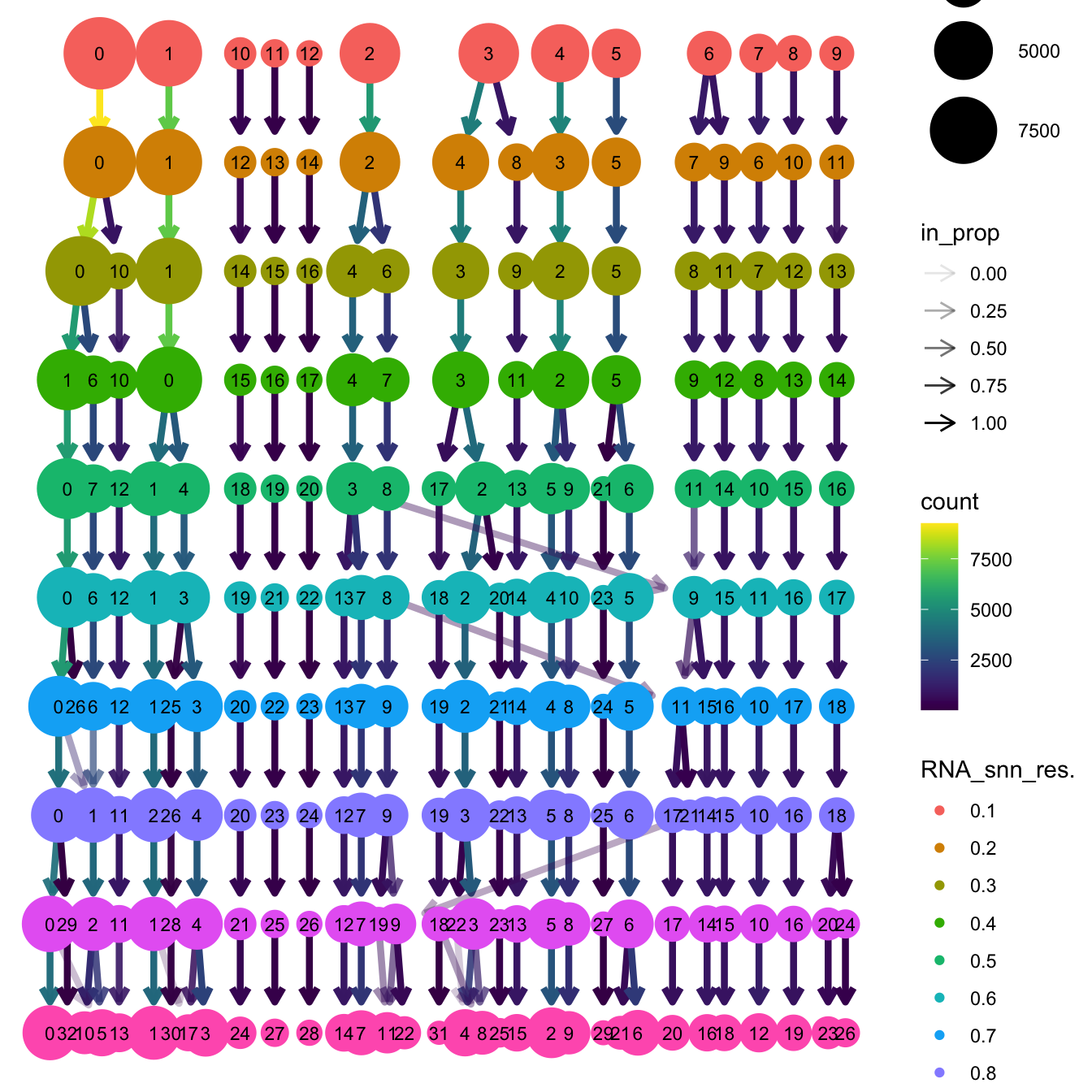
| Version | Author | Date |
|---|---|---|
| eebc9b9 | Gunjan Dixit | 2024-12-22 |
Based on the clustering tree, we chose an intermediate/optimum resolution where the clustering results are the most stable, with the least amount of shuffling cells.
opt_res <- "RNA_snn_res.0.5"
n <- nlevels(seu_obj$RNA_snn_res.0.5)
seu_obj$RNA_snn_res.0.5 <- factor(seu_obj$RNA_snn_res.0.5, levels = seq(0,n-1))
seu_obj$seurat_clusters <- NULL
seu_obj$cluster <- seu_obj$RNA_snn_res.0.5
Idents(seu_obj) <- seu_obj$cluster
UMAP after clustering
Defining colours for each cell-type to be consistent with other age-related/cell type composition plots.
my_colors <- c(
  "B cells" = "steelblue",
  "CD4 T cells" = "brown",
  "Double negative T cells" = "gold",
  "CD8 T cells" = "lightgreen",
  "Pre B/T cells" = "orchid",
  "Innate lymphoid cells" = "tan",
  "Natural Killer cells" = "blueviolet",
  "Macrophages" = "green4",
  "Cycling T cells" = "turquoise",
  "Dendritic cells" = "grey80",
  "Gamma delta T cells" = "mediumvioletred",
  "Epithelial lineage" = "darkorange",
  "Granulocytes" = "olivedrab",
  "Fibroblast lineage" = "lavender",
  "None" = "white",
  "Monocytes" = "peachpuff",
  "Endothelial lineage" = "cadetblue",
  "SMG duct" = "lightpink",
  "Neuroendocrine" = "skyblue",
  "Doublet query/Other" = "#d62728"
)
UMAP displaying clusters at opt_res resolution and Broad
cell Labels Level 3.
p1 <- DimPlot(seu_obj, reduction = "umap", raster = FALSE ,repel = TRUE, label = TRUE,label.size = 3.5, group.by = opt_res) +  NoLegend()

p2 <- DimPlot(seu_obj, reduction = "umap", raster = FALSE, repel = TRUE, label = TRUE, label.size = 3.5, group.by = "Broad_cell_label_3") + NoLegend() +
  scale_colour_manual(values = my_colors) +
  ggtitle(paste0(tissue, ": UMAP"))


p1 / p2 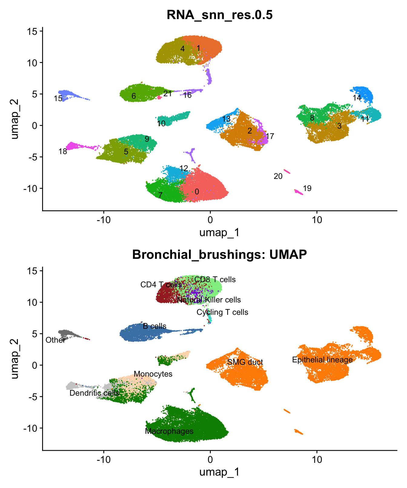
| Version | Author | Date |
|---|---|---|
| eebc9b9 | Gunjan Dixit | 2024-12-22 |
Save batch corrected Object
out1 <- here("output",
            "RDS", "AllBatches_Clustering_SEUs_v2",
             paste0("G000231_Neeland_",tissue,".Clusters.SEU.rds"))
#dir.create(out1)
if (!file.exists(out1)) {
  saveRDS(seu_obj, file = out1)
}
Marker Gene Analysis
The marker genes for this reclustering can be found here-
#seu_obj <- JoinLayers(seu_obj)
paed.markers <- FindAllMarkers(seu_obj, only.pos = TRUE, min.pct = 0.25, logfc.threshold = 0.25)
Extracting top 5 genes per cluster for visualization. The ‘top5’ contains the top 5 genes with the highest weighted average avg_log2FC within each cluster and the ‘best.wilcox.gene.per.cluster’ contains the single best gene with the highest weighted average avg_log2FC for each cluster.
paed.markers %>%
    group_by(cluster) %>% unique() %>%
    top_n(n = 5, wt = avg_log2FC) -> top5

paed.markers %>%
    group_by(cluster) %>%
    slice_head(n=1) %>%
    pull(gene) -> best.wilcox.gene.per.cluster

best.wilcox.gene.per.cluster
[1] "VSIG4" "CCL5" "KRT7" "CTXN1" "SPOCK2" "SPHK1"
[7] "CD79A" "CXCL3" "CTXN1" "APOBEC3A" "CSF3R" "PPIL6"
[13] "APOE" "PTGFR" "PTGFR" "CPA3" "UHRF1" "GPRC5A"
[19] "LILRA4" "KRT13" "ASCL3" "MZB1" Marker gene expression in clusters
This heatmap depicts the expression of top five genes in each cluster.
DoHeatmap(seu_obj, features = top5$gene) + NoLegend()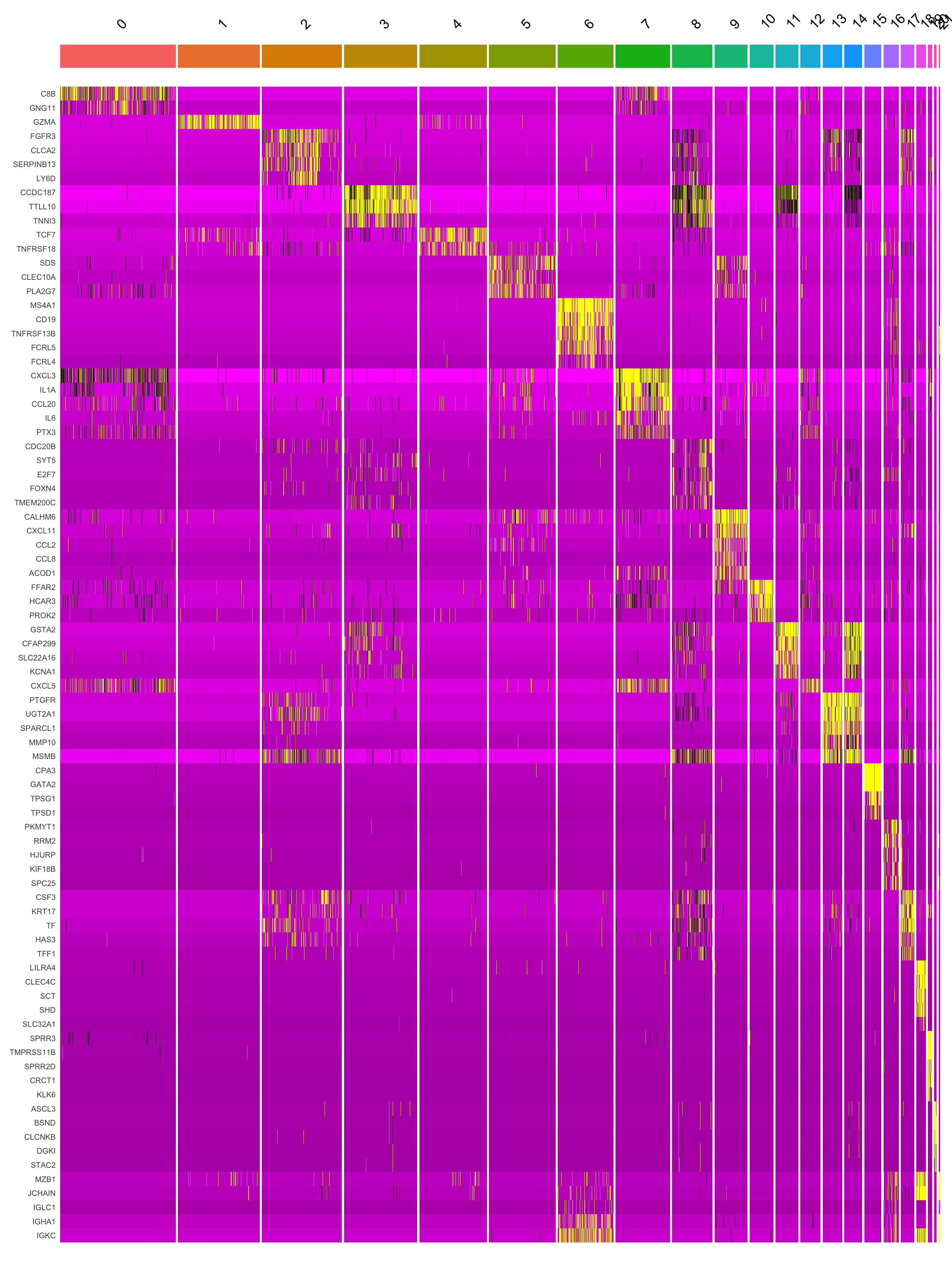
| Version | Author | Date |
|---|---|---|
| eebc9b9 | Gunjan Dixit | 2024-12-22 |
Violin plot shows the expression of top marker gene per cluster.
VlnPlot(seu_obj, features=best.wilcox.gene.per.cluster, ncol = 2, raster = FALSE, pt.size = FALSE)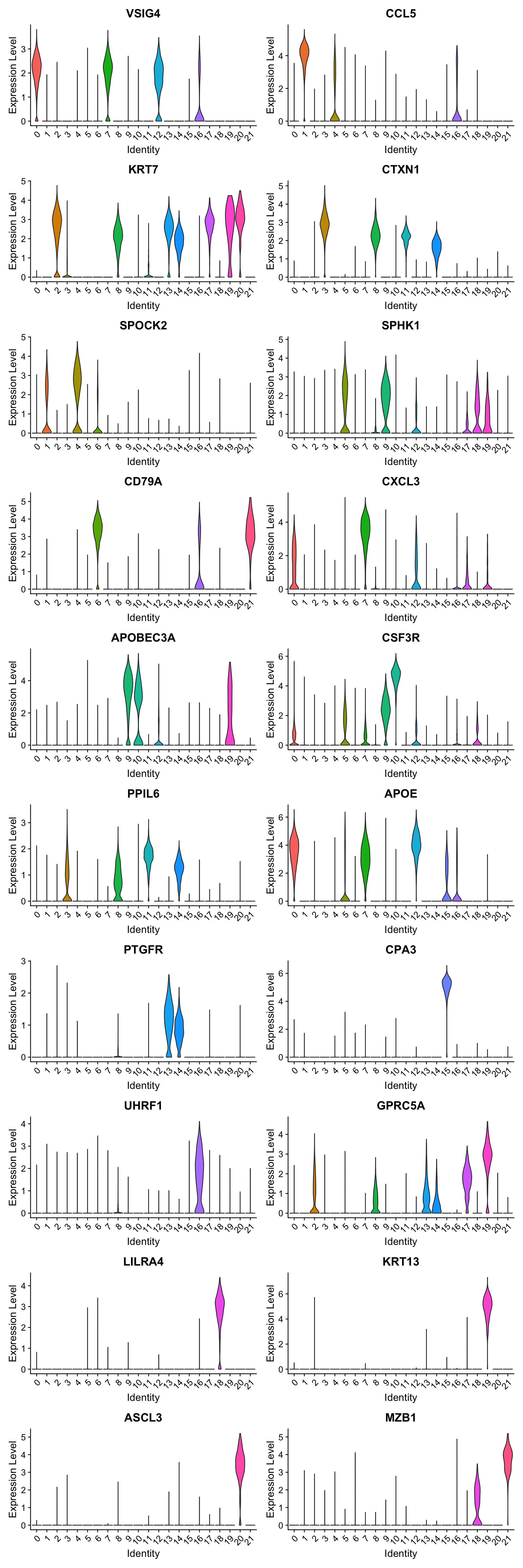
| Version | Author | Date |
|---|---|---|
| eebc9b9 | Gunjan Dixit | 2024-12-22 |
Feature plot shows the expression of top marker genes per cluster.
FeaturePlot(seu_obj,features=best.wilcox.gene.per.cluster, reduction = 'umap', raster = FALSE, ncol = 2)
| Version | Author | Date |
|---|---|---|
| eebc9b9 | Gunjan Dixit | 2024-12-22 |
Extract markers for each cluster
This section extracts marker genes for each cluster and save them as a CSV file.
out_markers <- here("output",
"CSV_v2", tissue,
paste(tissue,"_Marker_gene_clusters.",opt_res, sep = ""))
dir.create(out_markers, recursive = TRUE, showWarnings = FALSE)
for (cl in unique(paed.markers$cluster)) {
cluster_data <- paed.markers %>% dplyr::filter(cluster == cl)
file_name <- here(out_markers, paste0("G000231_Neeland_",tissue, "_cluster_", cl, ".csv"))
write.csv(cluster_data, file = file_name)
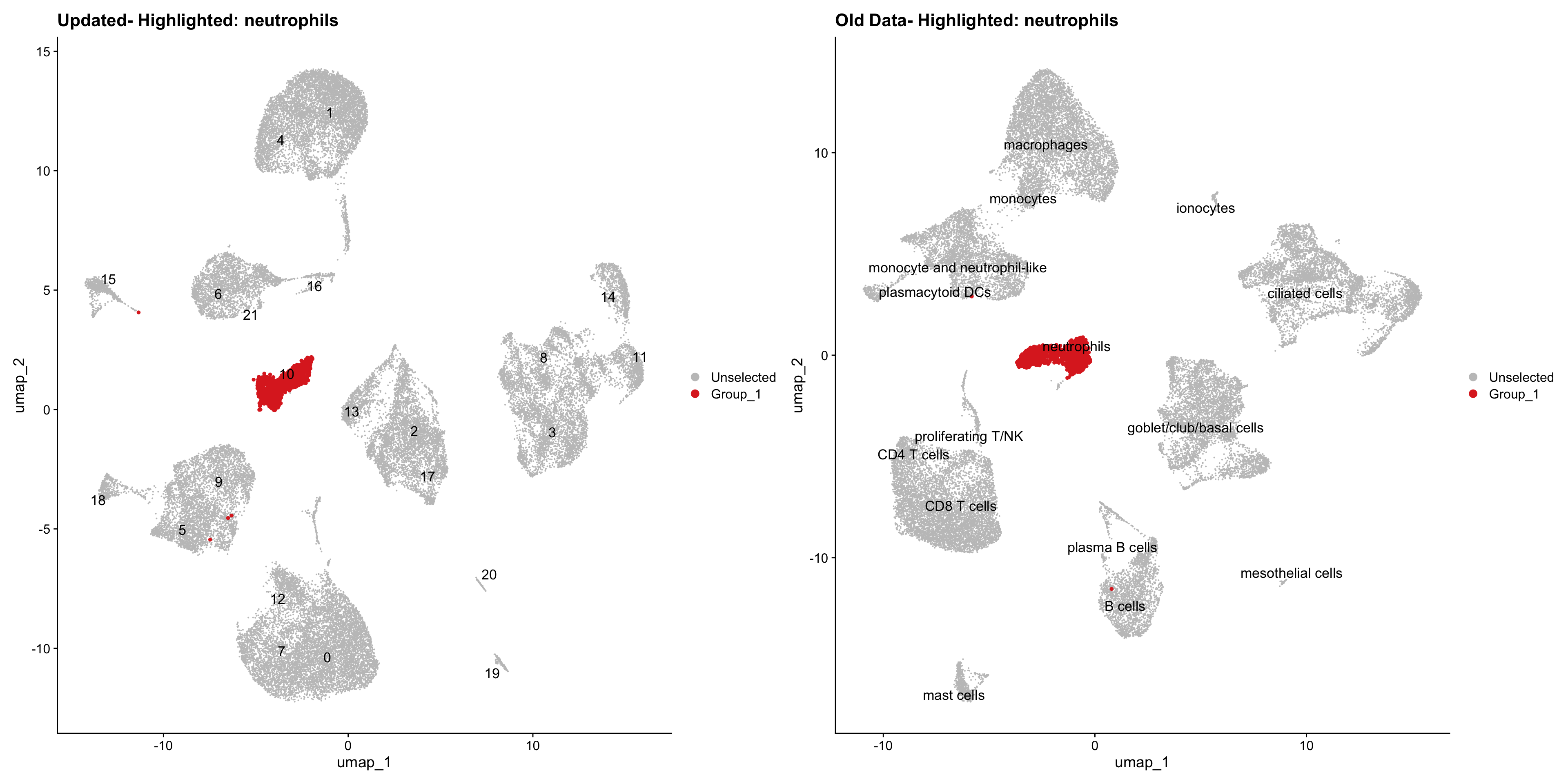
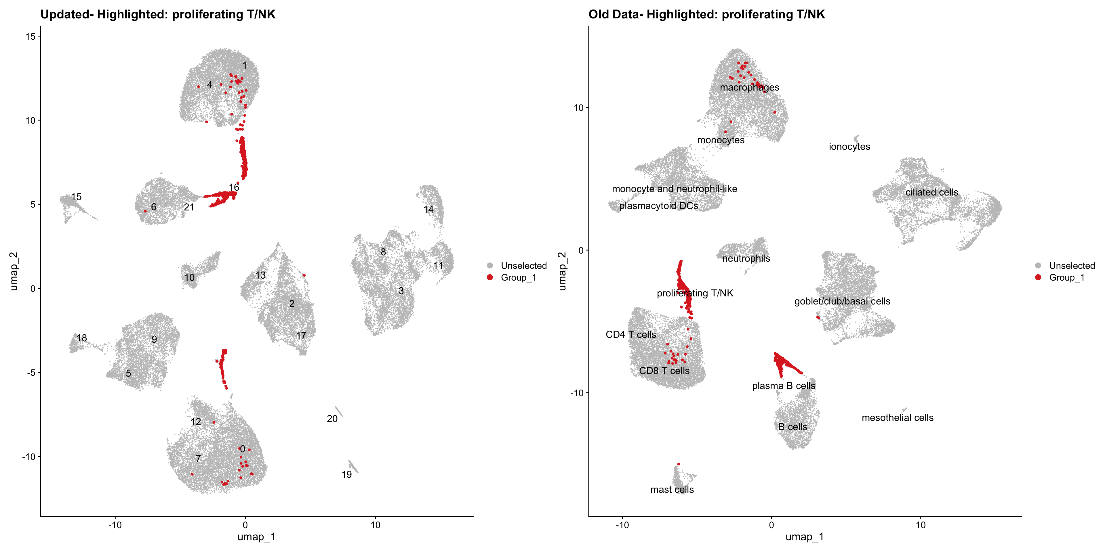
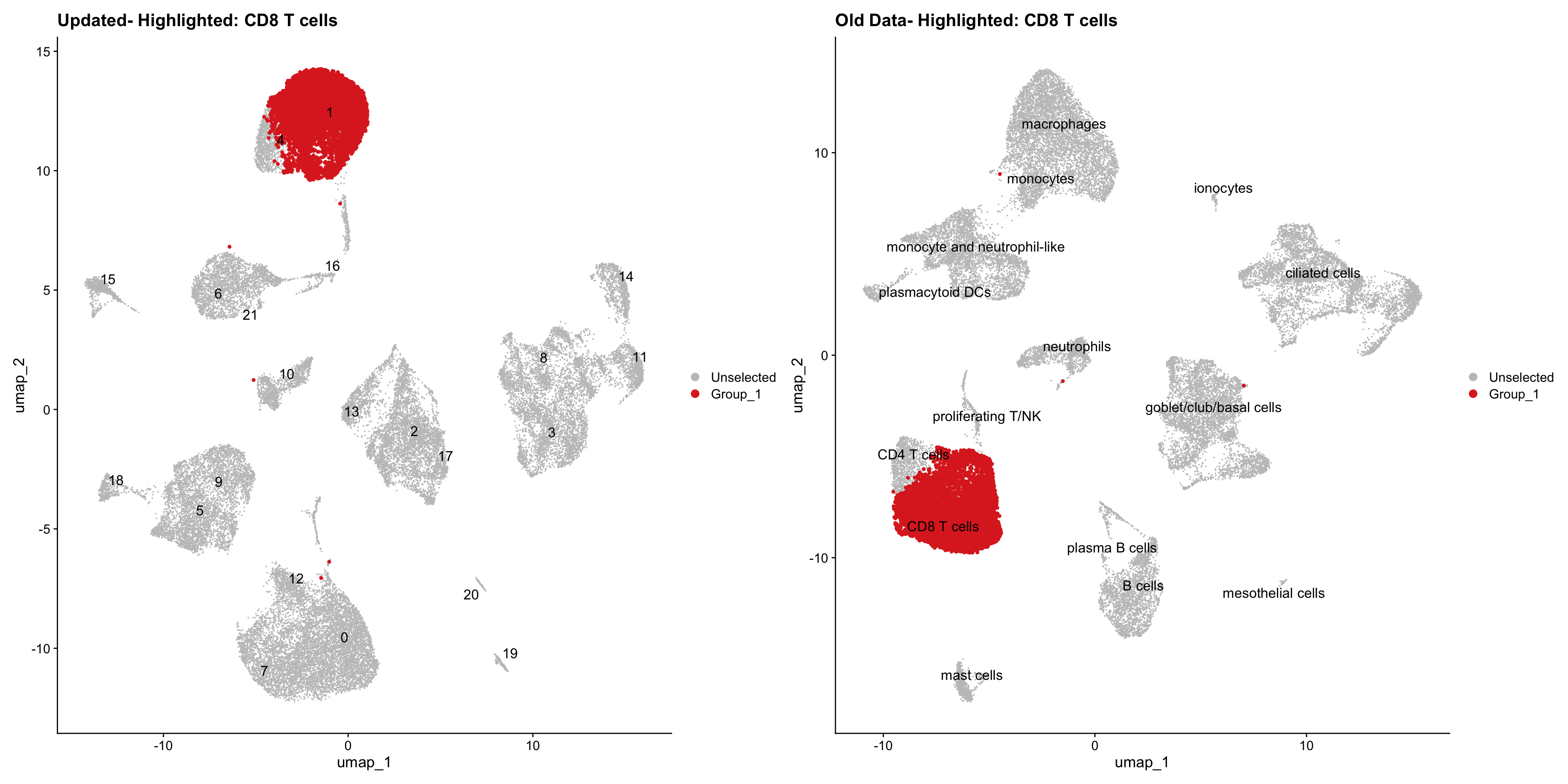
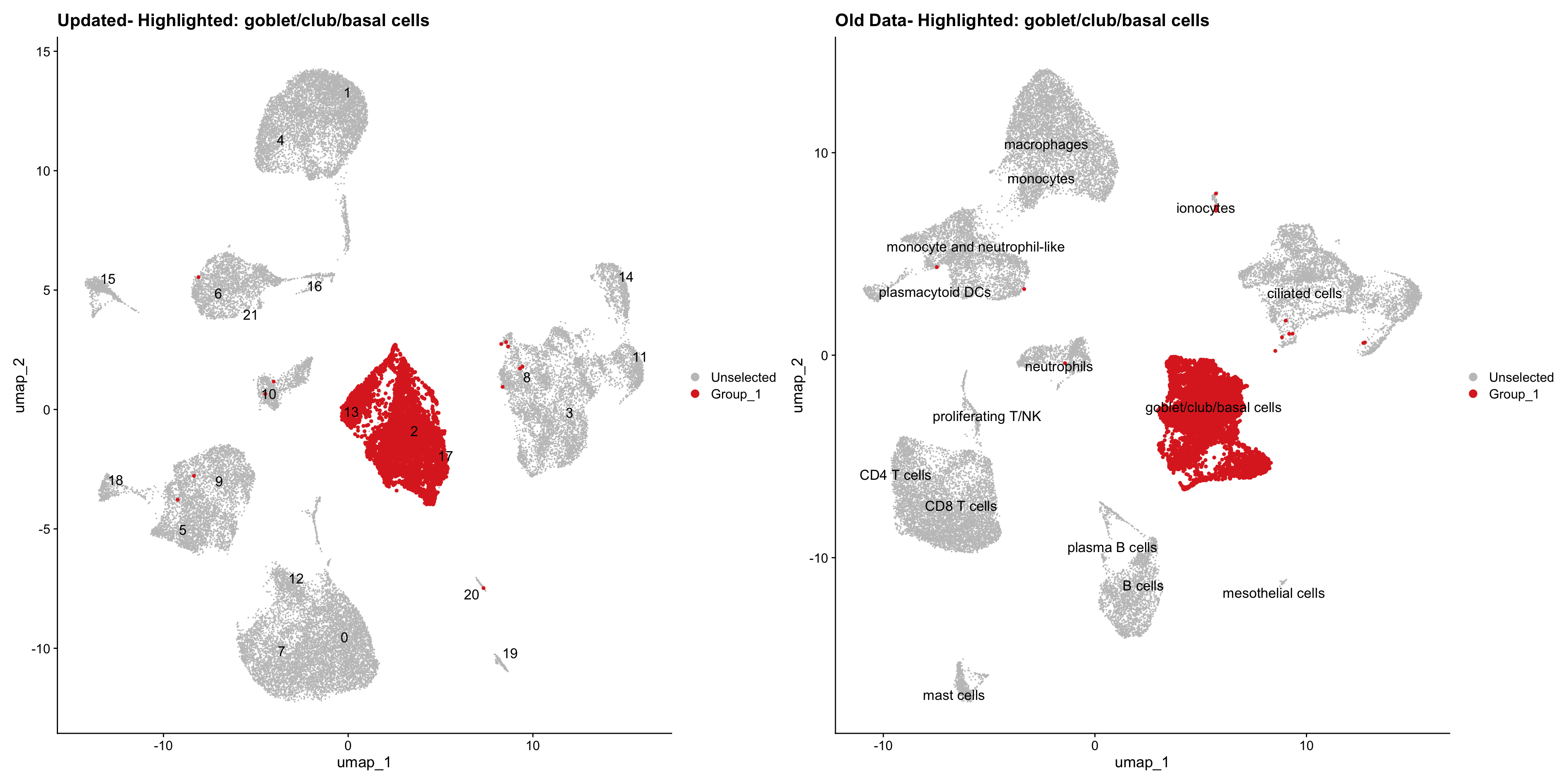
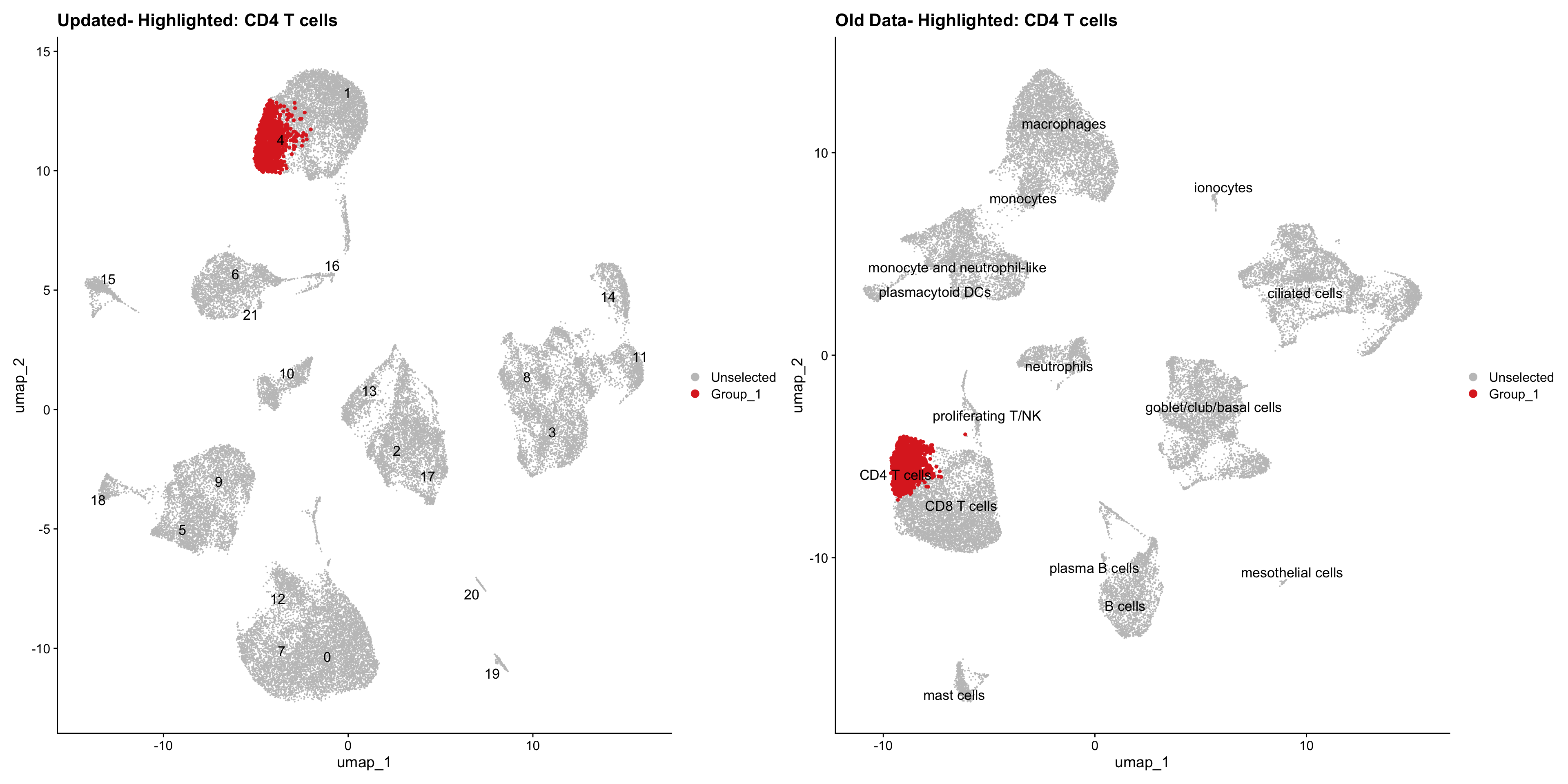
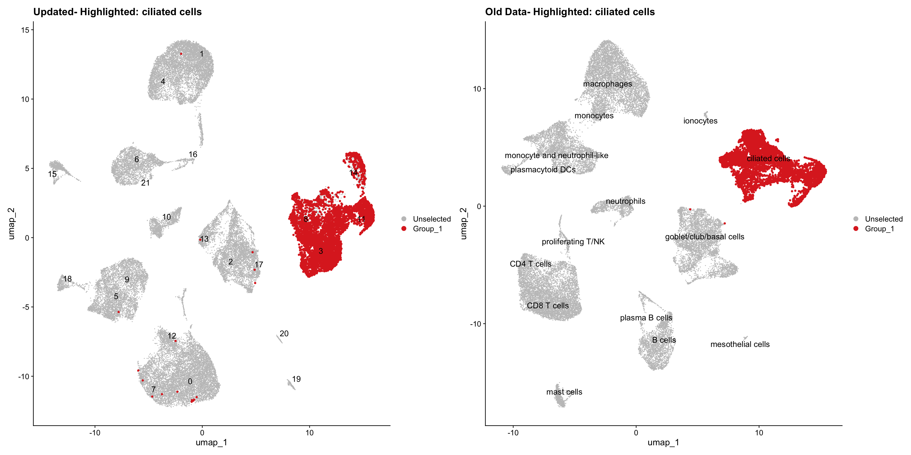
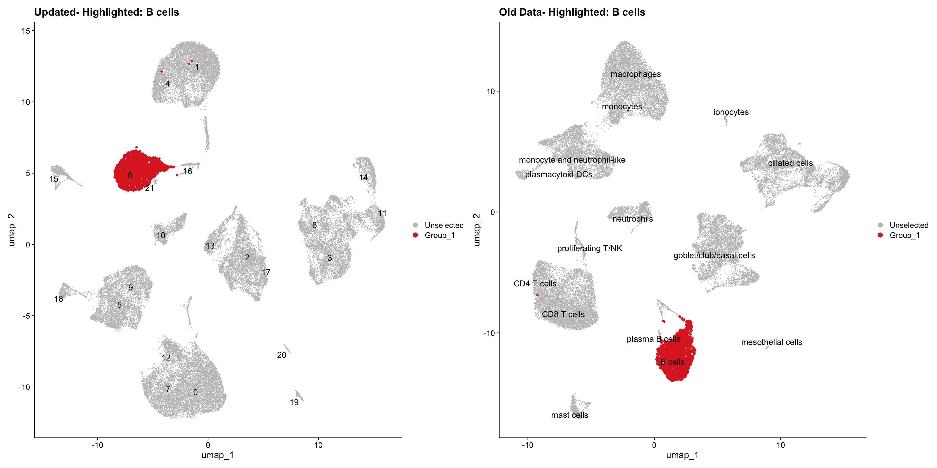
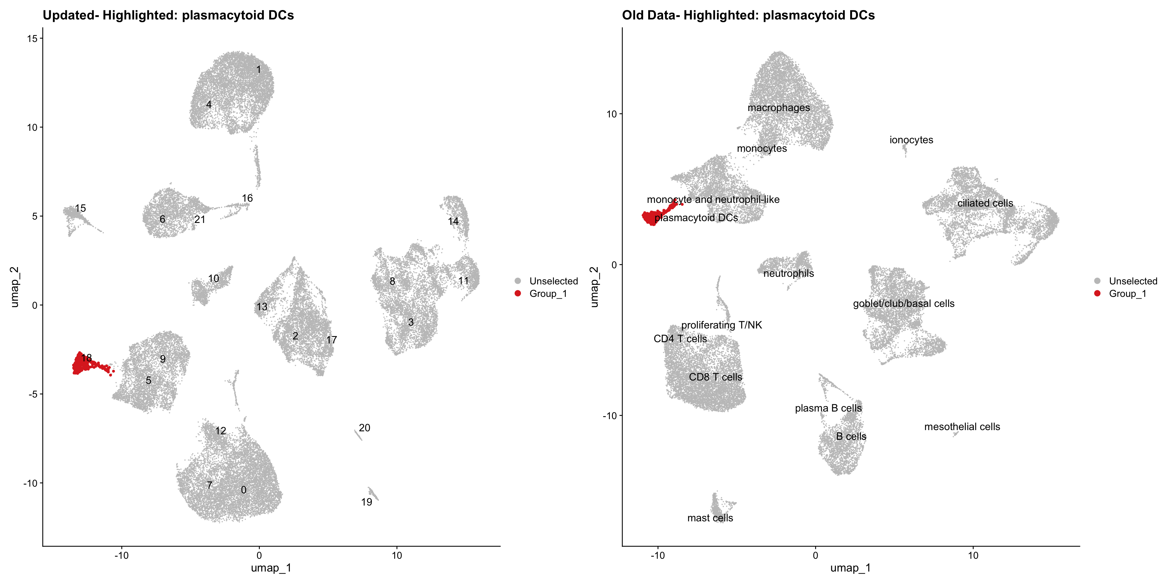
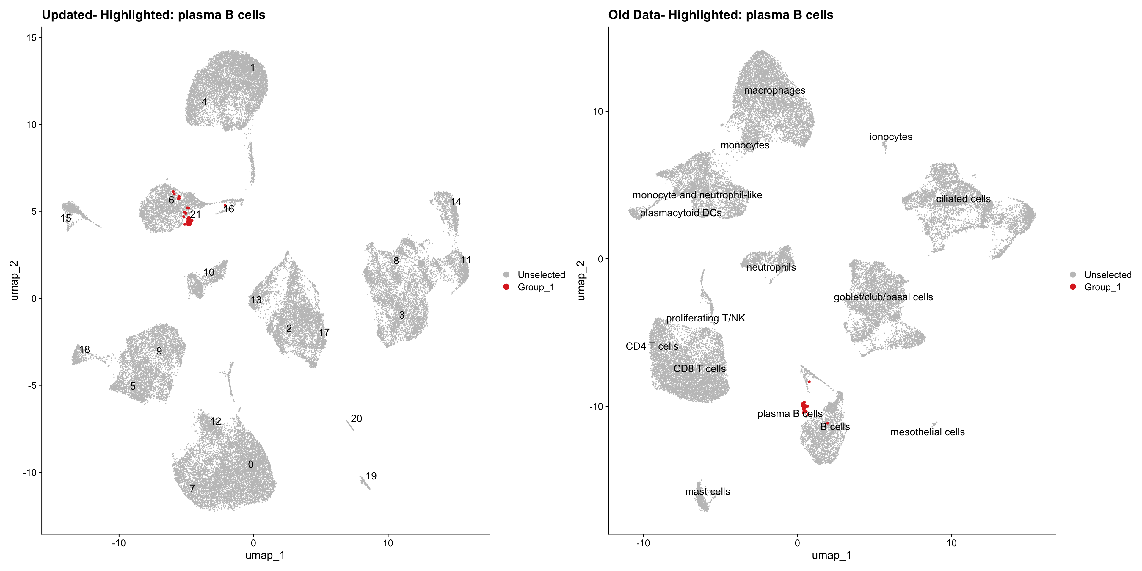
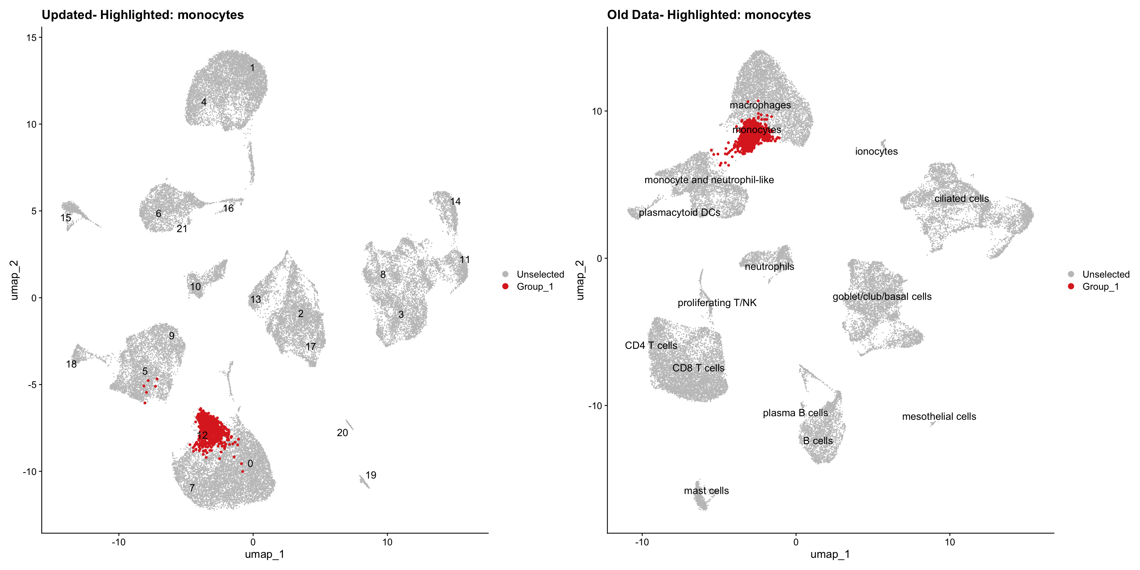
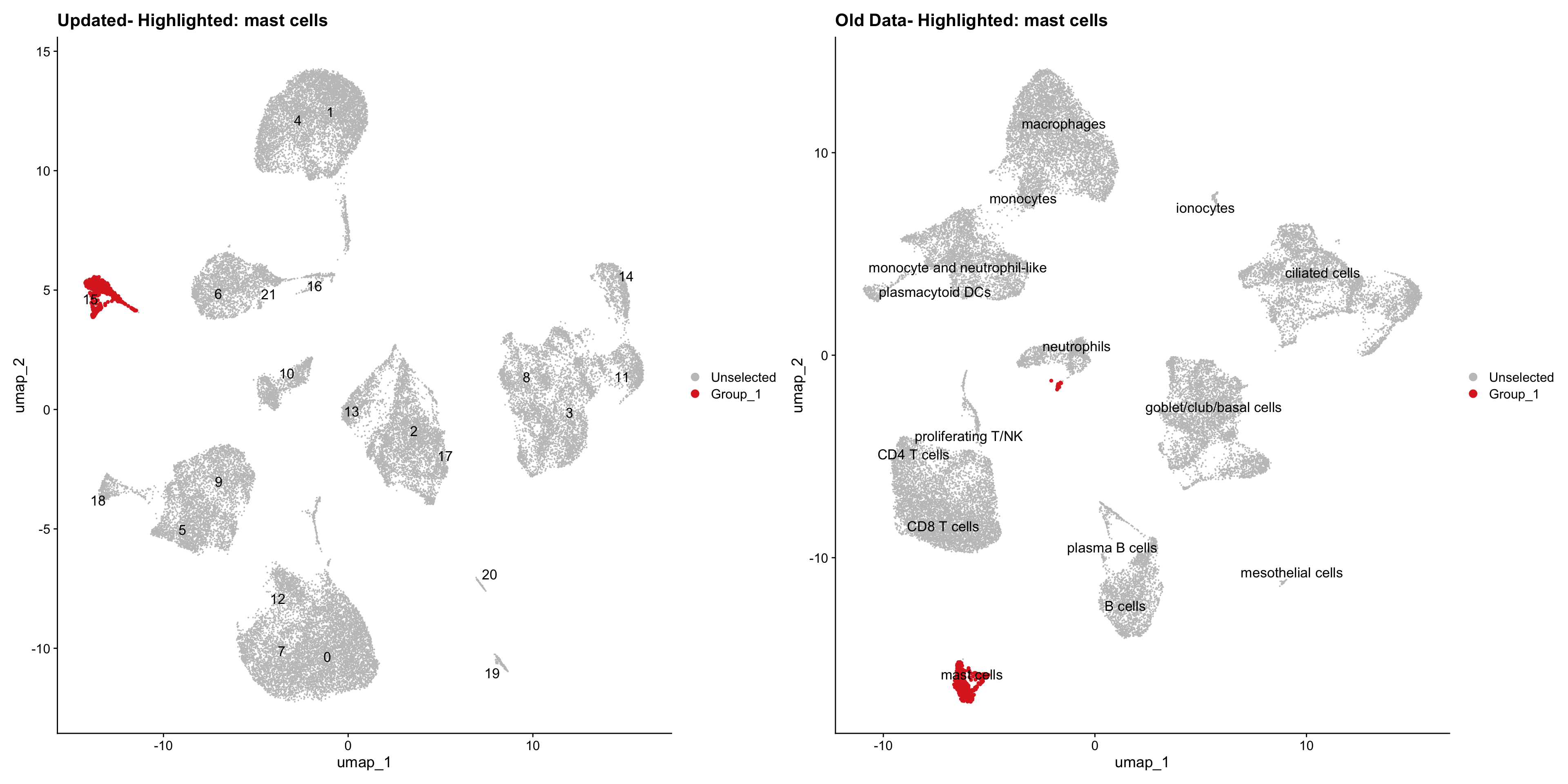
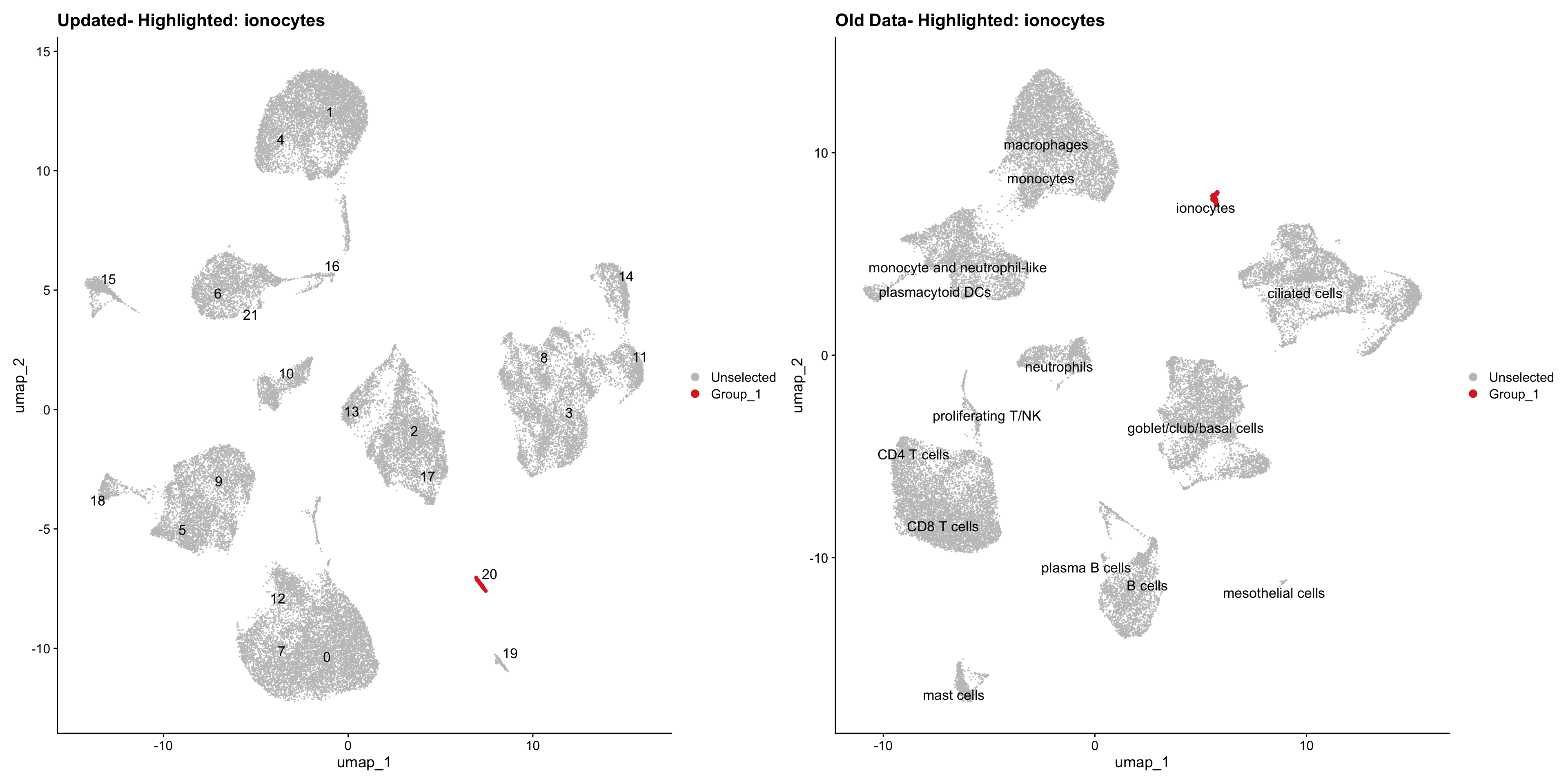
}Using old labels to annotate cell types
out1 <- here("output",
            "RDS", "AllBatches_Clustering_SEUs",
             paste0("G000231_Neeland_",tissue,".Clusters.SEU.rds"))
old_obj <- readRDS(out1)
cell_types <- unique(old_obj$cell_labels)
for (cell_type in cell_types) {
cl_cells <- WhichCells(old_obj, idents = cell_type)
p <- DimPlot(
seu_obj,
reduction = "umap",
label = TRUE,
label.size = 4.5,
repel = TRUE,
raster = FALSE,
cells.highlight = cl_cells
) +
ggtitle(paste("Updated- Highlighted:", cell_type))
p1 <- DimPlot(
old_obj,
reduction = "umap",
label = T,
label.size = 4.5,
repel = TRUE,
raster = FALSE,
cells.highlight = cl_cells
) +
ggtitle(paste("Old Data- Highlighted:", cell_type))
print(p | p1)
}
| Version | Author | Date |
|---|---|---|
| eebc9b9 | Gunjan Dixit | 2024-12-22 |
| Version | Author | Date |
|---|---|---|
| eebc9b9 | Gunjan Dixit | 2024-12-22 |
| Version | Author | Date |
|---|---|---|
| eebc9b9 | Gunjan Dixit | 2024-12-22 |
| Version | Author | Date |
|---|---|---|
| eebc9b9 | Gunjan Dixit | 2024-12-22 |
| Version | Author | Date |
|---|---|---|
| eebc9b9 | Gunjan Dixit | 2024-12-22 |
| Version | Author | Date |
|---|---|---|
| eebc9b9 | Gunjan Dixit | 2024-12-22 |
| Version | Author | Date |
|---|---|---|
| eebc9b9 | Gunjan Dixit | 2024-12-22 |
| Version | Author | Date |
|---|---|---|
| eebc9b9 | Gunjan Dixit | 2024-12-22 |
| Version | Author | Date |
|---|---|---|
| eebc9b9 | Gunjan Dixit | 2024-12-22 |
| Version | Author | Date |
|---|---|---|
| eebc9b9 | Gunjan Dixit | 2024-12-22 |
| Version | Author | Date |
|---|---|---|
| eebc9b9 | Gunjan Dixit | 2024-12-22 |
| Version | Author | Date |
|---|---|---|
| eebc9b9 | Gunjan Dixit | 2024-12-22 |
| Version | Author | Date |
|---|---|---|
| eebc9b9 | Gunjan Dixit | 2024-12-22 |
| Version | Author | Date |
|---|---|---|
| eebc9b9 | Gunjan Dixit | 2024-12-22 |
| Version | Author | Date |
|---|---|---|
| eebc9b9 | Gunjan Dixit | 2024-12-22 |
Updated cell-type labels (all clusters)
cell_labels <- readxl::read_excel(here("data/cell_labels_Mel_v4_Dec2024/earlyAIR_BB_all.xlsx"), sheet = "all_clusters")

new_cluster_names <- cell_labels %>%
  dplyr::select(cluster, annotation) %>%
  deframe()

seu_obj <- RenameIdents(seu_obj, new_cluster_names)
seu_obj@meta.data$cell_labels <- Idents(seu_obj)

p3 <- DimPlot(seu_obj, reduction = "umap", raster = FALSE, repel = TRUE, label = TRUE, label.size = 3.5) + ggtitle(paste0(tissue, ": UMAP with Updated cell types"))

p3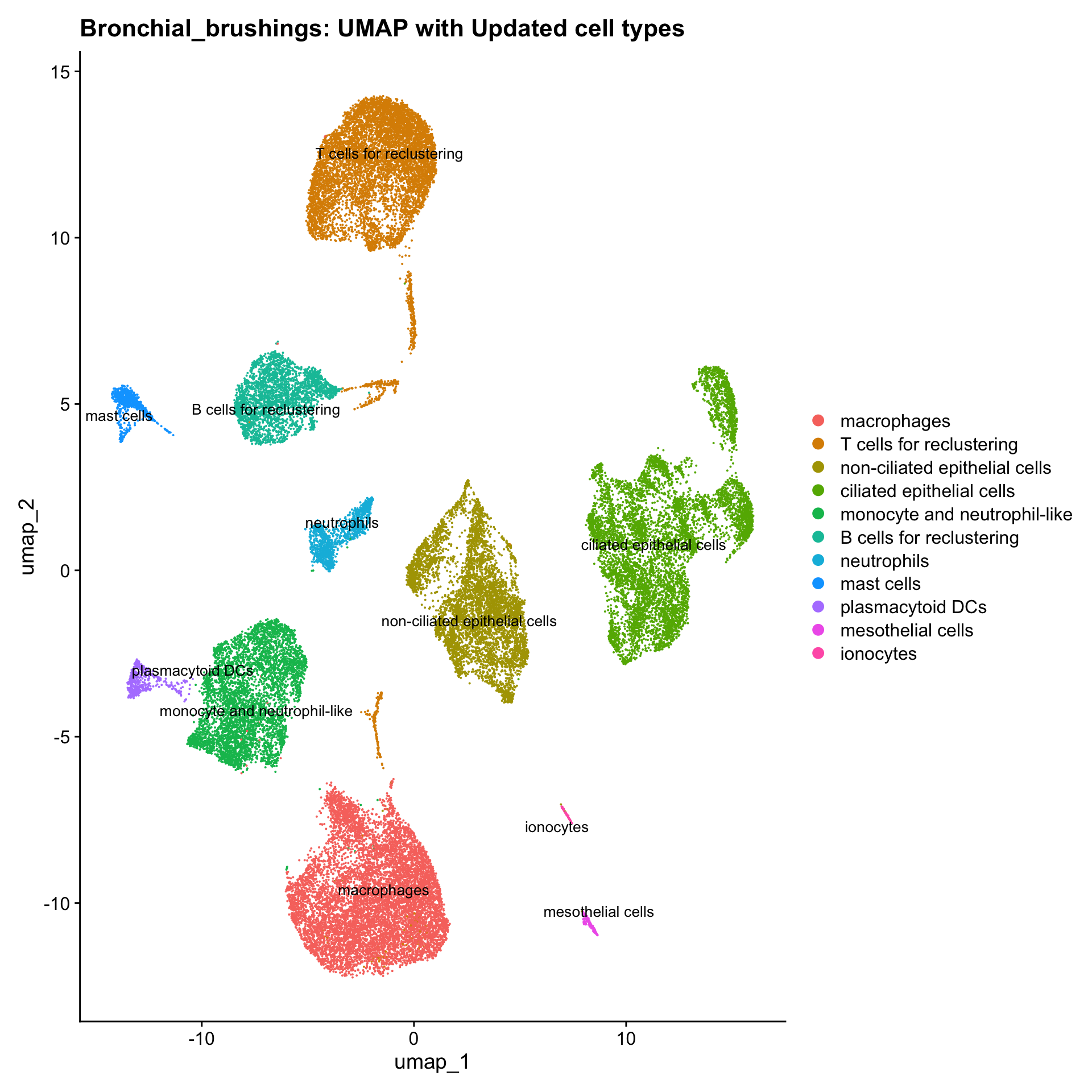
| Version | Author | Date |
|---|---|---|
| 3595ad0 | Gunjan Dixit | 2025-01-07 |
Reclustering T cell population
This includes CD4 T cell, CD8 T cell, NK cell, NK-T cell, proliferating or cycling T/NK cell.
The marker genes for this reclustering can be found here-
sub_clusters <- c(1, 4, 16)
idx <- which(seu_obj$cluster %in% sub_clusters)

paed_sub <- seu_obj[,idx]
mito_genes <- grep("^MT-", rownames(paed_sub), value = TRUE)
paed_sub <- subset(paed_sub, features = setdiff(rownames(paed_sub), mito_genes))
paed_sub
An object of class Seurat
18035 features across 7941 samples within 1 assay
Active assay: RNA (18035 features, 1997 variable features)
3 layers present: counts, data, scale.data
2 dimensional reductions calculated: pca, umappaed_sub <- paed_sub %>%
NormalizeData() %>%
FindVariableFeatures() %>%
ScaleData() %>%
RunPCA()
paed_sub <- RunUMAP(paed_sub, dims = 1:30, reduction = "pca", reduction.name = "umap.tcell")
meta_data <- colnames(paed_sub@meta.data)
drop <- grep("^RNA_snn_res", meta_data, value = TRUE)
paed_sub@meta.data <- paed_sub@meta.data[, !(colnames(paed_sub@meta.data) %in% drop)]
resolutions <- seq(0.1, 1, by = 0.1)
paed_sub <- FindNeighbors(paed_sub, reduction = "pca", dims = 1:30)
paed_sub <- FindClusters(paed_sub, resolution = resolutions, algorithm = 3)Modularity Optimizer version 1.3.0 by Ludo Waltman and Nees Jan van Eck
Number of nodes: 7941
Number of edges: 293472
Running smart local moving algorithm...
Maximum modularity in 10 random starts: 0.9396
Number of communities: 6
Elapsed time: 4 seconds
Modularity Optimizer version 1.3.0 by Ludo Waltman and Nees Jan van Eck
Number of nodes: 7941
Number of edges: 293472
Running smart local moving algorithm...
Maximum modularity in 10 random starts: 0.9138
Number of communities: 9
Elapsed time: 3 seconds
Modularity Optimizer version 1.3.0 by Ludo Waltman and Nees Jan van Eck
Number of nodes: 7941
Number of edges: 293472
Running smart local moving algorithm...
Maximum modularity in 10 random starts: 0.8950
Number of communities: 10
Elapsed time: 3 seconds
Modularity Optimizer version 1.3.0 by Ludo Waltman and Nees Jan van Eck
Number of nodes: 7941
Number of edges: 293472
Running smart local moving algorithm...
Maximum modularity in 10 random starts: 0.8805
Number of communities: 12
Elapsed time: 3 seconds
Modularity Optimizer version 1.3.0 by Ludo Waltman and Nees Jan van Eck
Number of nodes: 7941
Number of edges: 293472
Running smart local moving algorithm...
Maximum modularity in 10 random starts: 0.8666
Number of communities: 14
Elapsed time: 3 seconds
Modularity Optimizer version 1.3.0 by Ludo Waltman and Nees Jan van Eck
Number of nodes: 7941
Number of edges: 293472
Running smart local moving algorithm...
Maximum modularity in 10 random starts: 0.8551
Number of communities: 15
Elapsed time: 3 seconds
Modularity Optimizer version 1.3.0 by Ludo Waltman and Nees Jan van Eck
Number of nodes: 7941
Number of edges: 293472
Running smart local moving algorithm...
Maximum modularity in 10 random starts: 0.8446
Number of communities: 16
Elapsed time: 3 seconds
Modularity Optimizer version 1.3.0 by Ludo Waltman and Nees Jan van Eck
Number of nodes: 7941
Number of edges: 293472
Running smart local moving algorithm...
Maximum modularity in 10 random starts: 0.8347
Number of communities: 17
Elapsed time: 3 seconds
Modularity Optimizer version 1.3.0 by Ludo Waltman and Nees Jan van Eck
Number of nodes: 7941
Number of edges: 293472
Running smart local moving algorithm...
Maximum modularity in 10 random starts: 0.8255
Number of communities: 17
Elapsed time: 3 seconds
Modularity Optimizer version 1.3.0 by Ludo Waltman and Nees Jan van Eck
Number of nodes: 7941
Number of edges: 293472
Running smart local moving algorithm...
Maximum modularity in 10 random starts: 0.8167
Number of communities: 20
Elapsed time: 3 secondsDimHeatmap(paed_sub, dims = 1:10, cells = 500, balanced = TRUE)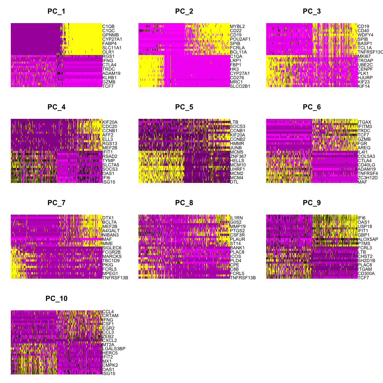
| Version | Author | Date |
|---|---|---|
| eebc9b9 | Gunjan Dixit | 2024-12-22 |
clustree(paed_sub, prefix = "RNA_snn_res.")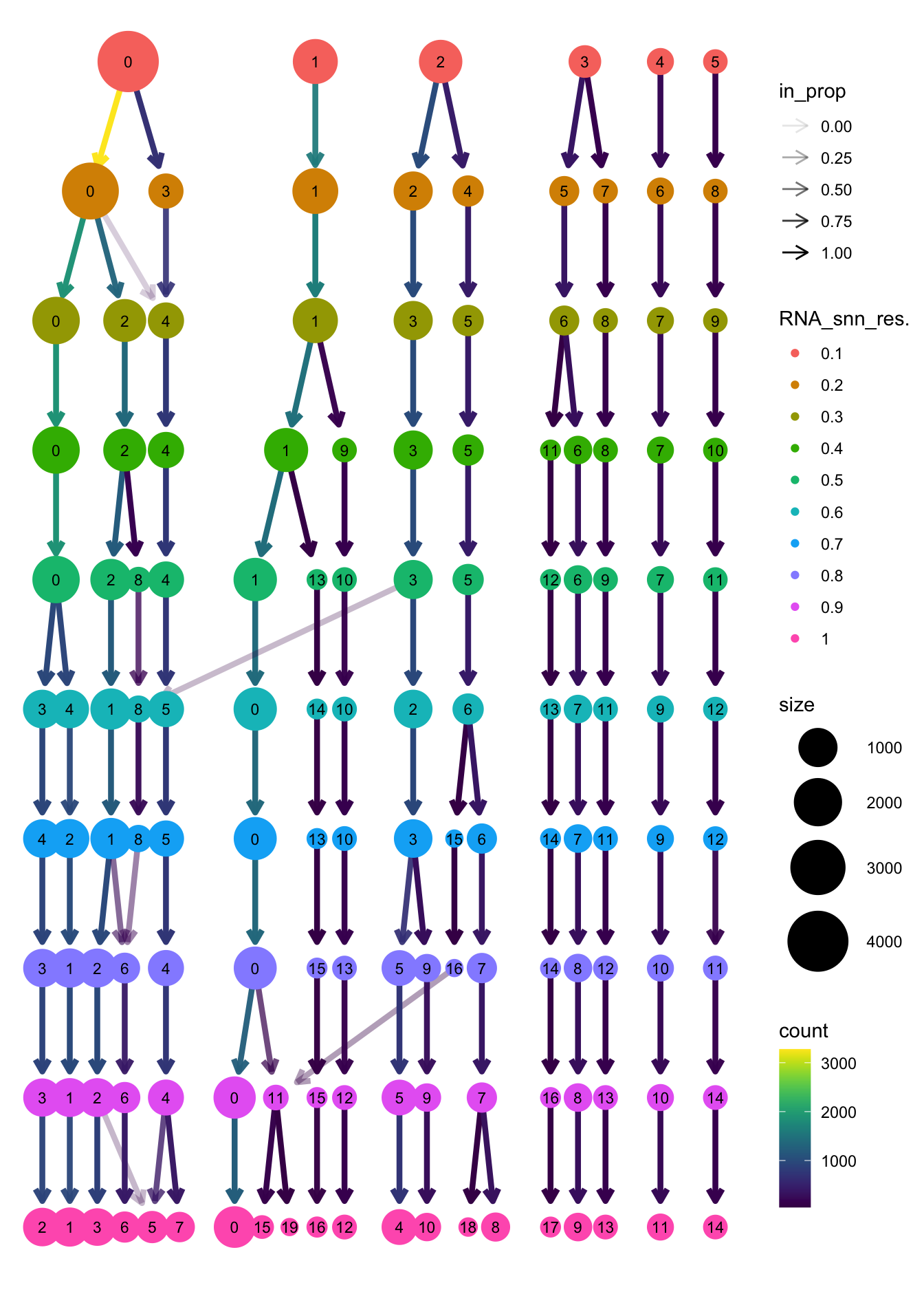
| Version | Author | Date |
|---|---|---|
| 3595ad0 | Gunjan Dixit | 2025-01-07 |
# Visualize the clustering results
DimPlot(paed_sub, group.by = "RNA_snn_res.0.5", reduction = "umap.tcell", label = TRUE, label.size = 2.5, repel = TRUE, raster = FALSE )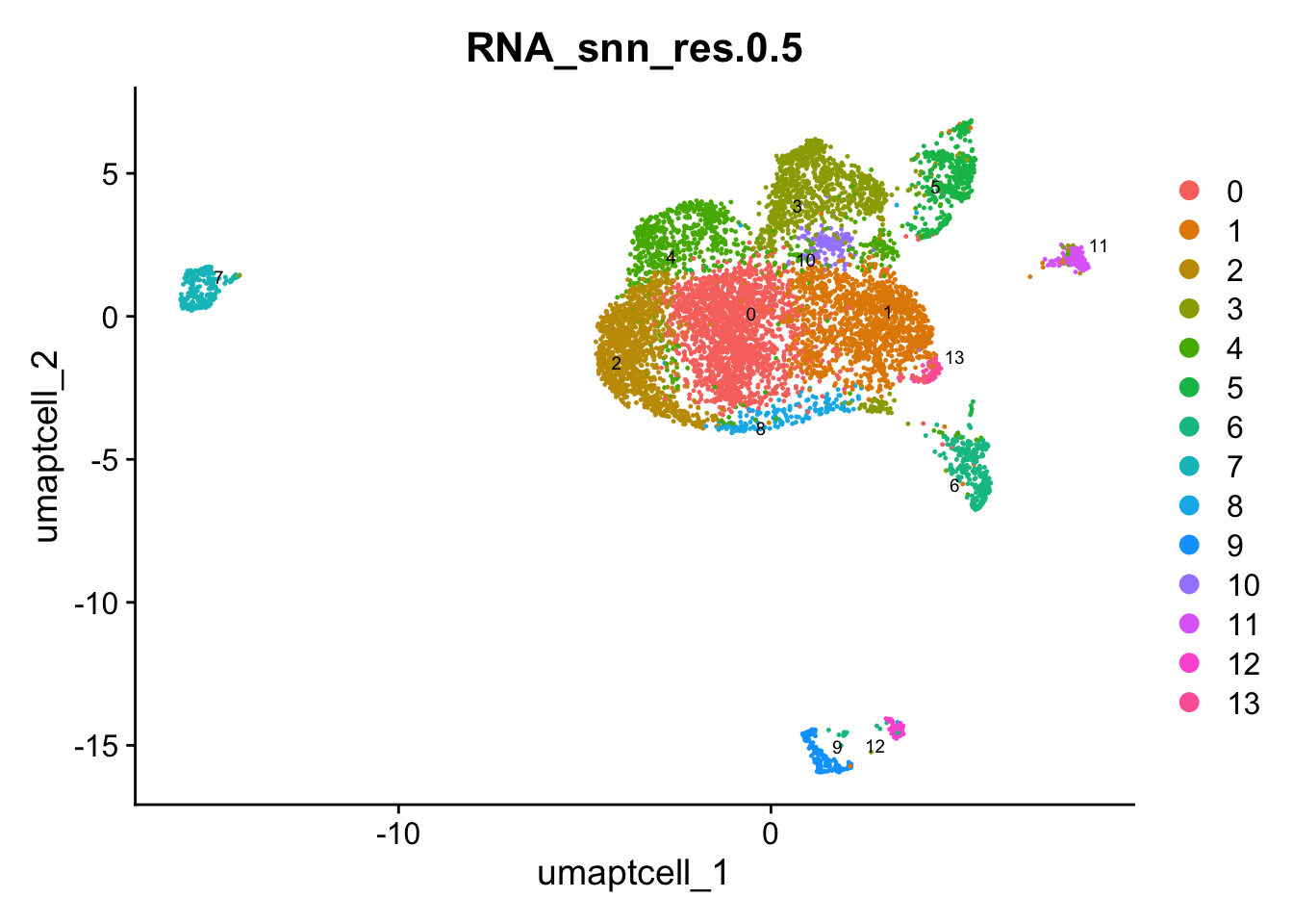
opt_res <- "RNA_snn_res.0.5"
n <- nlevels(paed_sub$RNA_snn_res.0.5)
paed_sub$RNA_snn_res.0.5 <- factor(paed_sub$RNA_snn_res.0.5, levels = seq(0,n-1))
paed_sub$seurat_clusters <- NULL
paed_sub$cluster <- paed_sub$RNA_snn_res.0.5
Idents(paed_sub) <- paed_sub$cluster
paed_sub.markers <- FindAllMarkers(paed_sub, only.pos = TRUE, min.pct = 0.25, logfc.threshold = 0.25)Calculating cluster 0Calculating cluster 1Calculating cluster 2Calculating cluster 3Calculating cluster 4Calculating cluster 5Calculating cluster 6Calculating cluster 7Calculating cluster 8Calculating cluster 9Calculating cluster 10Calculating cluster 11Calculating cluster 12Calculating cluster 13paed_sub.markers %>%
group_by(cluster) %>% unique() %>%
top_n(n = 5, wt = avg_log2FC) -> top5
paed_sub.markers %>%
group_by(cluster) %>%
slice_head(n=1) %>%
pull(gene) -> best.wilcox.gene.per.cluster
best.wilcox.gene.per.cluster [1] "CCL5" "MAF" "CCL5" "TCF7" "LAG3" "TYROBP" "UHRF1"
[8] "ALDH2" "CCL4L2" "POU2AF1" "NOG" "CSF3R" "SPIB" "HSPA1B" Feature plot shows the expression of top marker genes per cluster.
FeaturePlot(paed_sub,features=best.wilcox.gene.per.cluster, reduction = 'umap.tcell', raster = FALSE, ncol = 2, label = TRUE)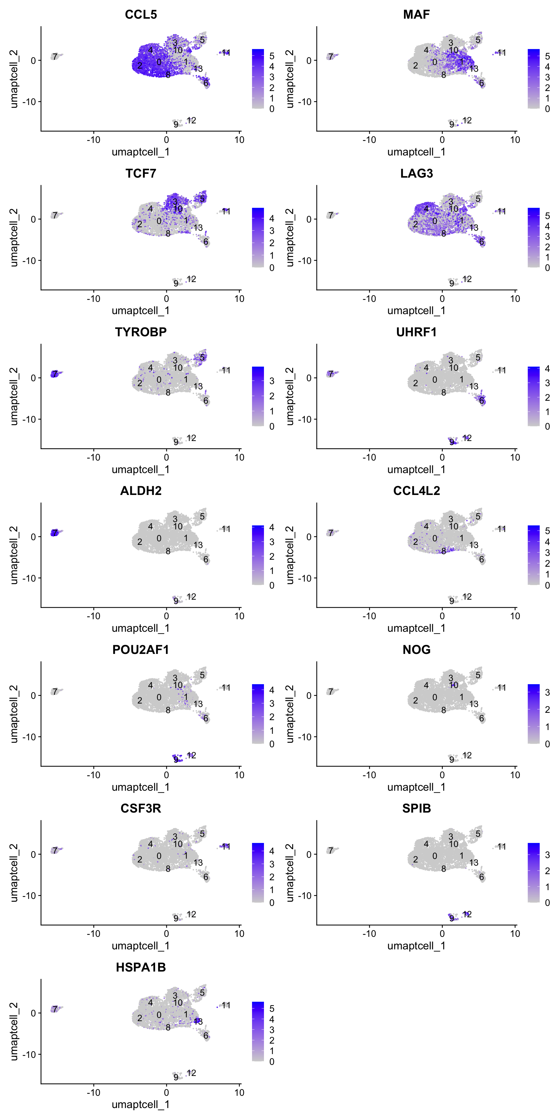
Top 10 marker genes from Seurat
## Seurat top markers
top10 <- paed_sub.markers %>%
    group_by(cluster) %>%
    top_n(n = 10, wt = avg_log2FC) %>%
    ungroup() %>%
    distinct(gene, .keep_all = TRUE) %>%
    arrange(cluster, desc(avg_log2FC))

cluster_colors <- paletteer::paletteer_d("pals::glasbey")[factor(top10$cluster)]

DotPlot(paed_sub,
        features = unique(top10$gene),
        group.by = opt_res,
        cols = c("azure1", "blueviolet"),
        dot.scale = 3, assay = "RNA") +
    RotatedAxis() +
    FontSize(y.text = 8, x.text = 12) +
    labs(y = element_blank(), x = element_blank()) +
    coord_flip() +
    theme(axis.text.y = element_text(color = cluster_colors)) +
    ggtitle("Top 10 marker genes per cluster (Seurat)")
Warning: Vectorized input to `element_text()` is not officially supported.
ℹ Results may be unexpected or may change in future versions of ggplot2.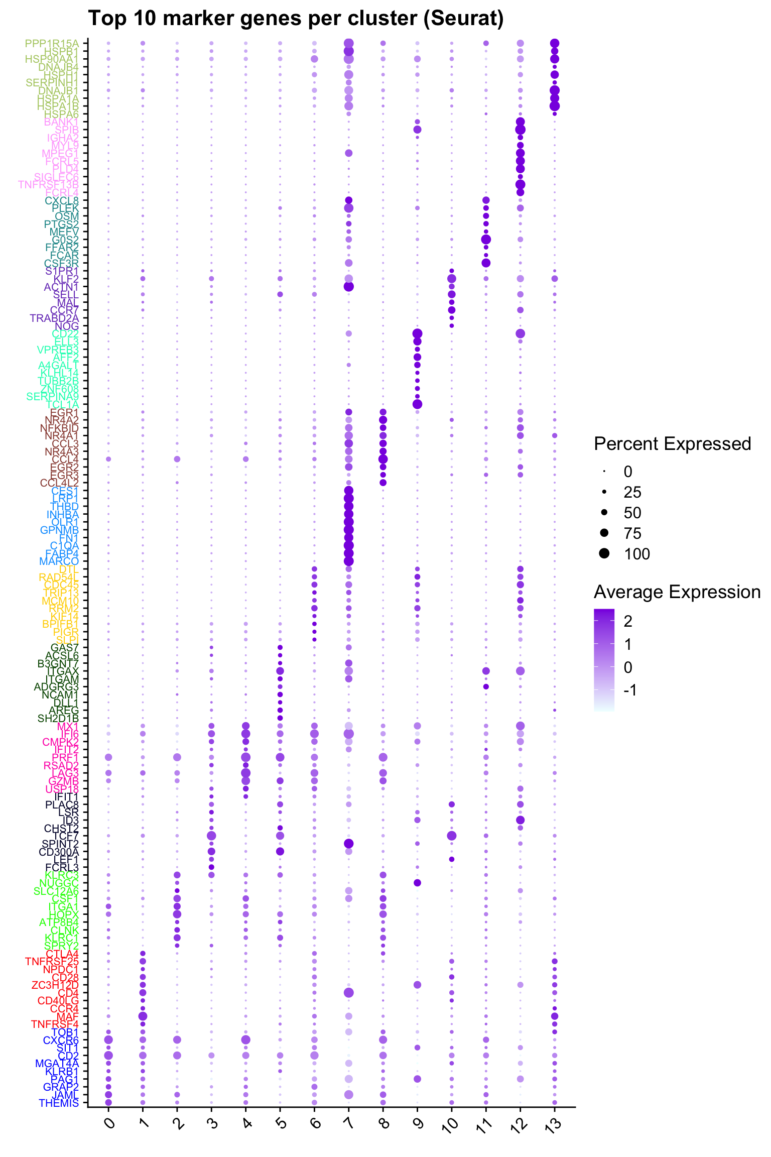
| Version | Author | Date |
|---|---|---|
| 3595ad0 | Gunjan Dixit | 2025-01-07 |
out_markers <- here("output",
"CSV_v2", tissue,
paste(tissue,"_Marker_genes_Reclustered_Tcell_population.",opt_res, sep = ""))
dir.create(out_markers, recursive = TRUE, showWarnings = FALSE)
for (cl in unique(paed_sub.markers$cluster)) {
cluster_data <- paed_sub.markers %>% dplyr::filter(cluster == cl)
file_name <- here(out_markers, paste0("G000231_Neeland_",tissue, "_cluster_", cl, ".csv"))
write.csv(cluster_data, file = file_name)
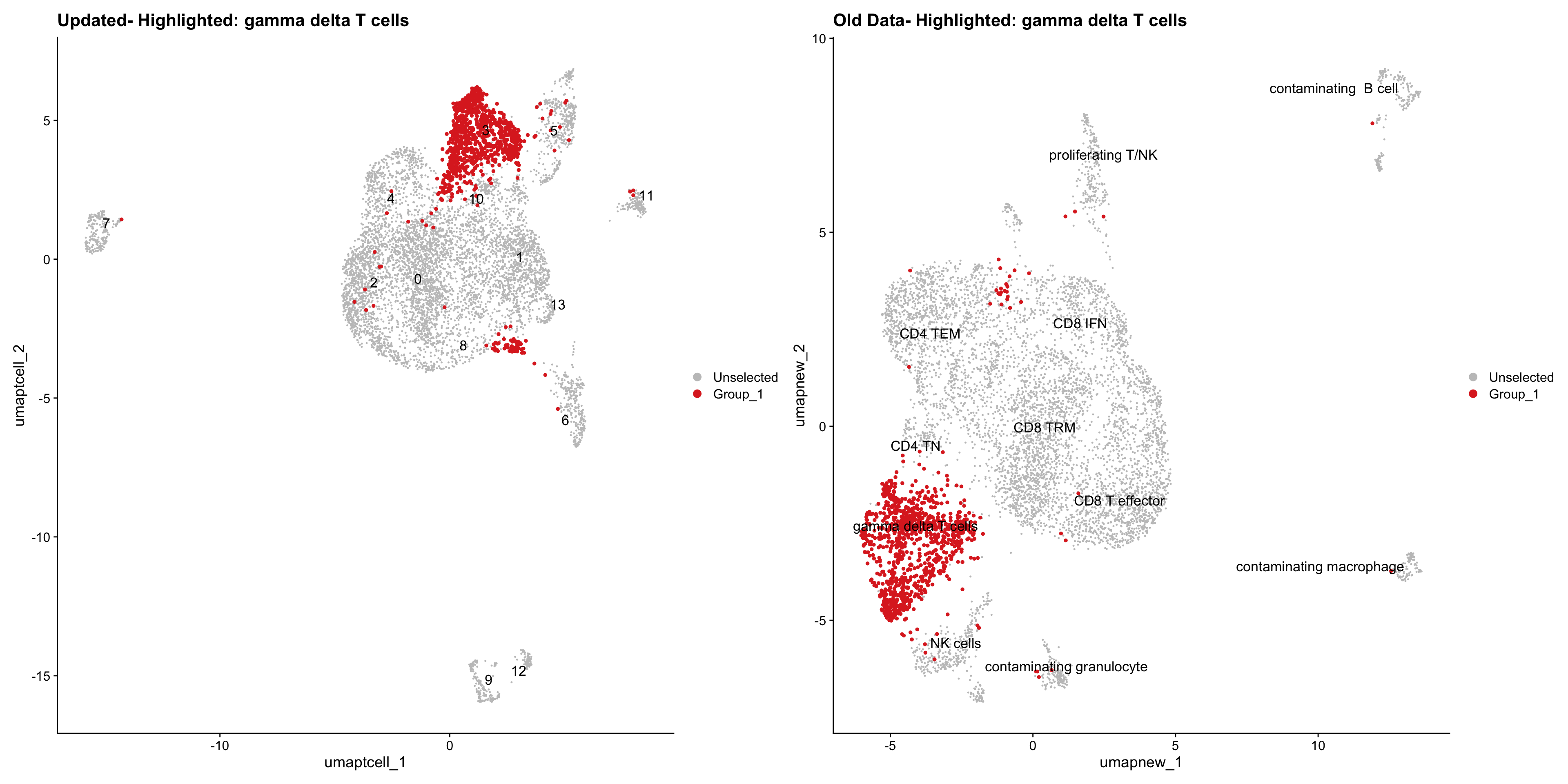
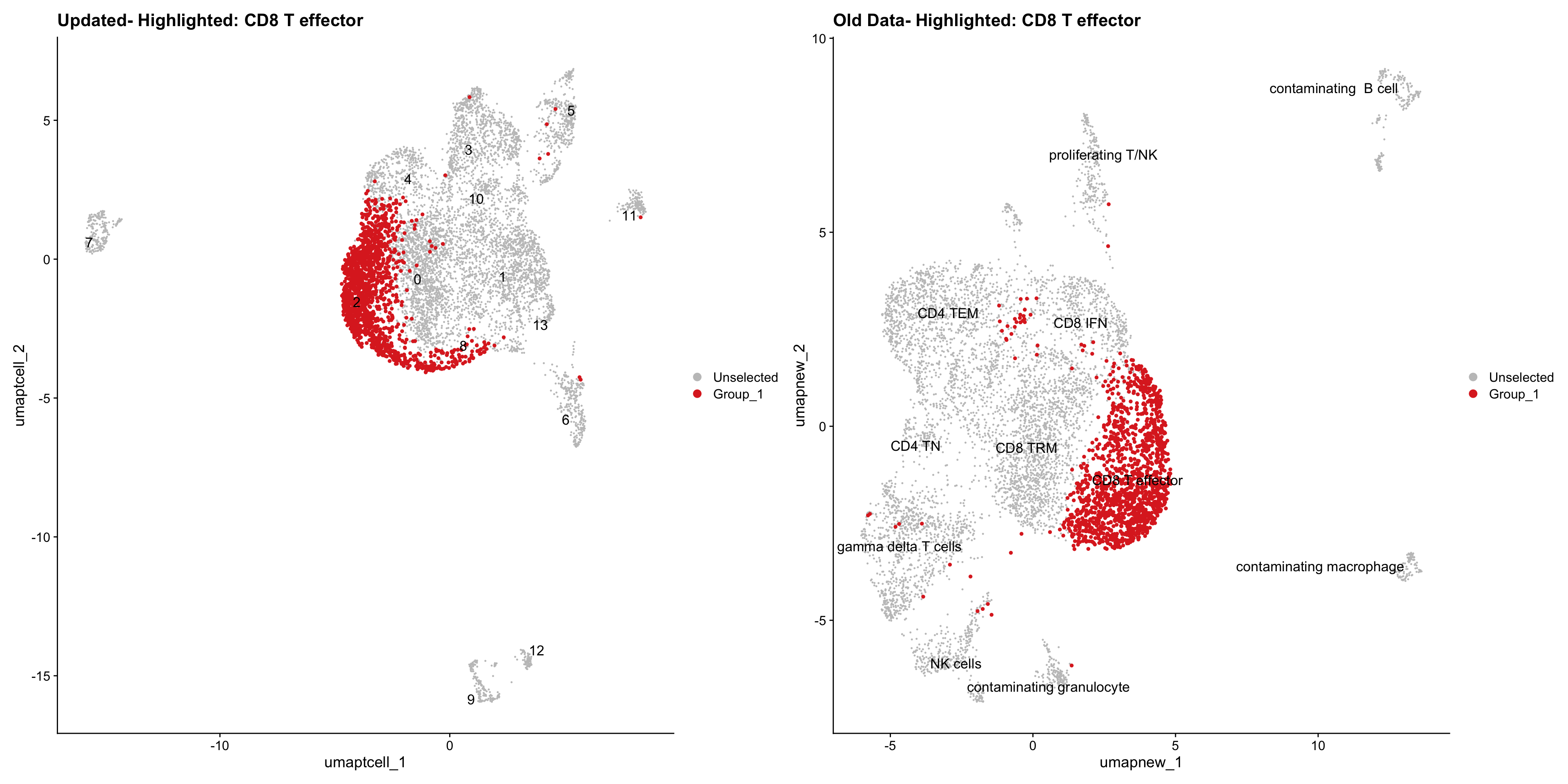
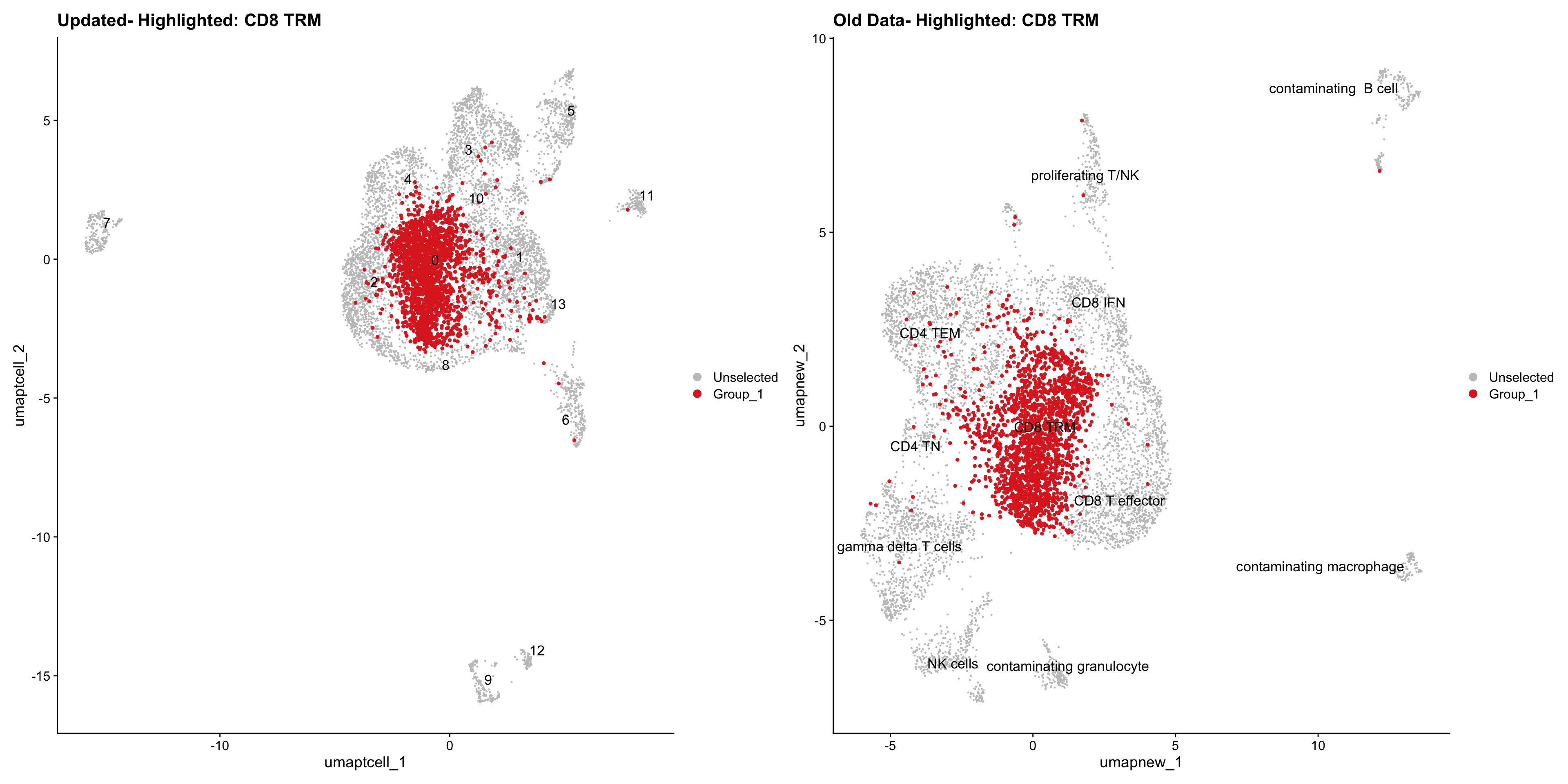
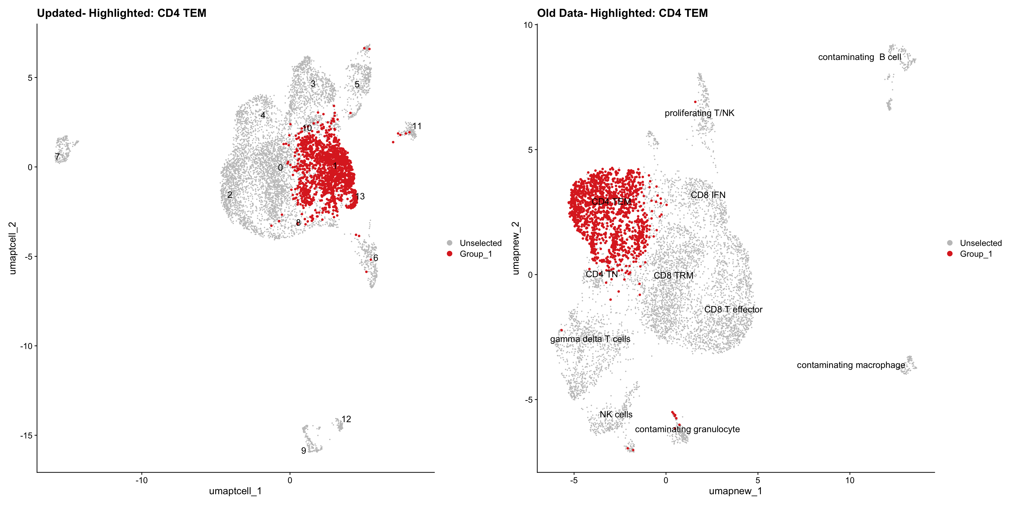
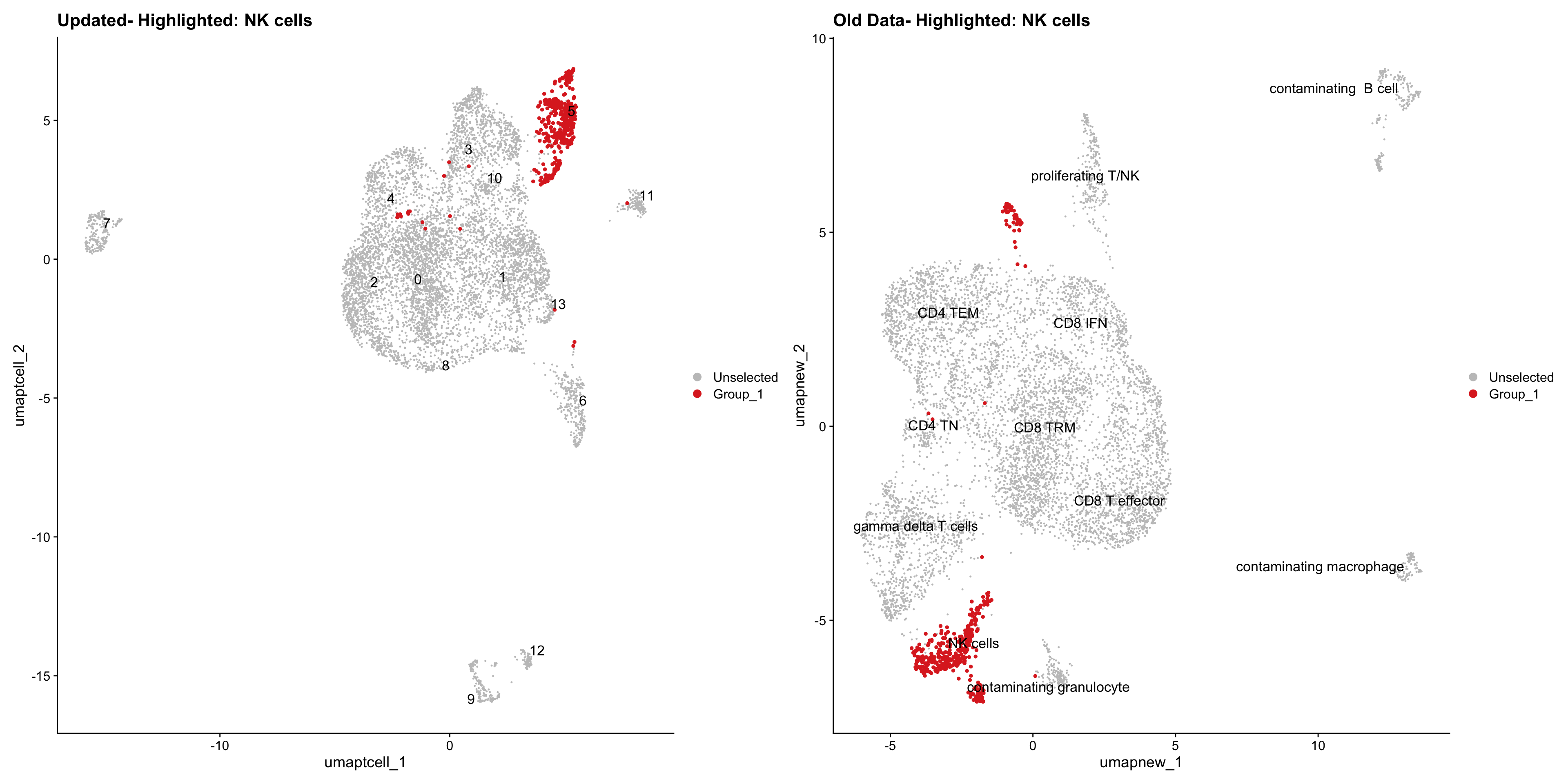
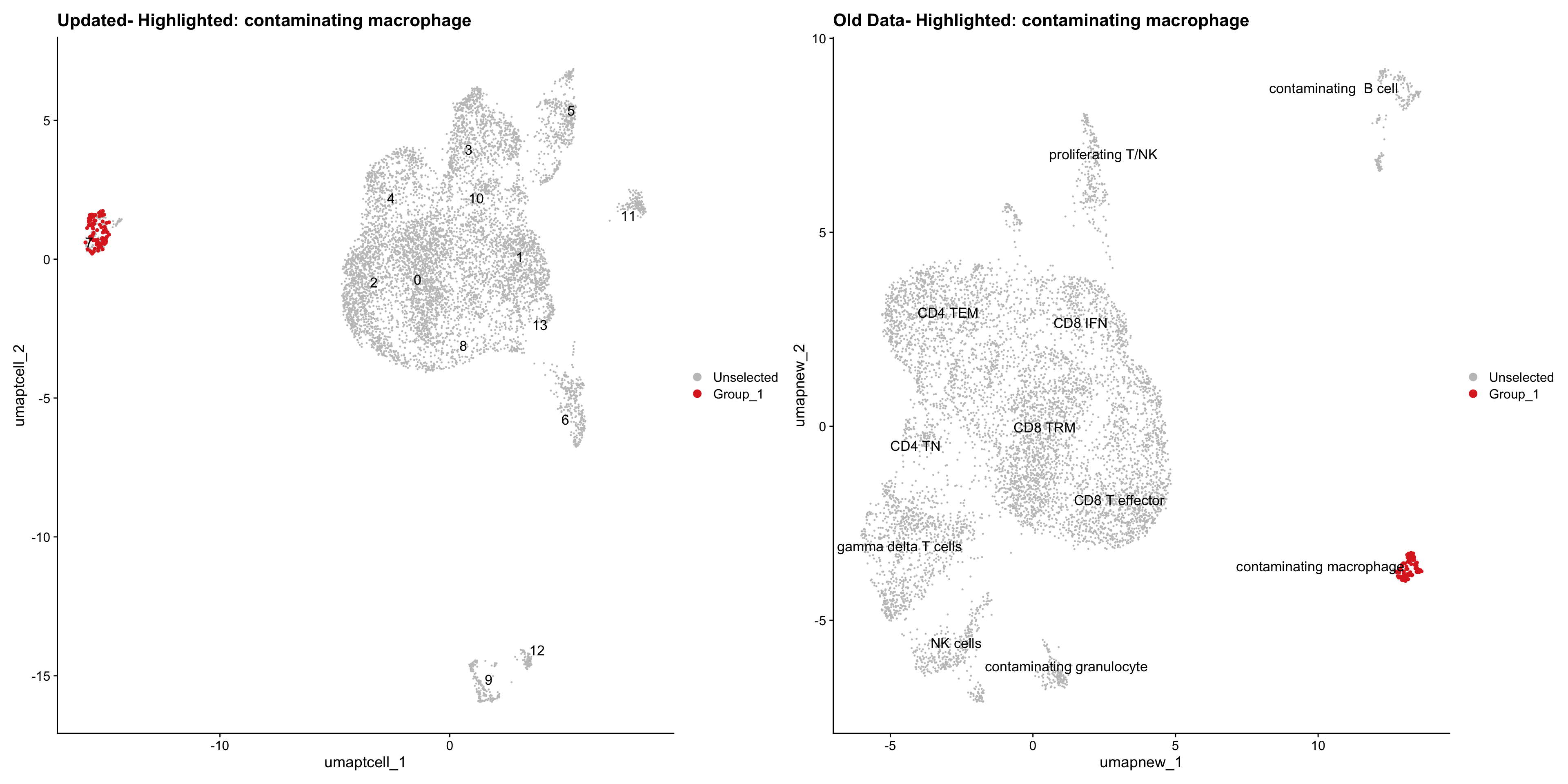
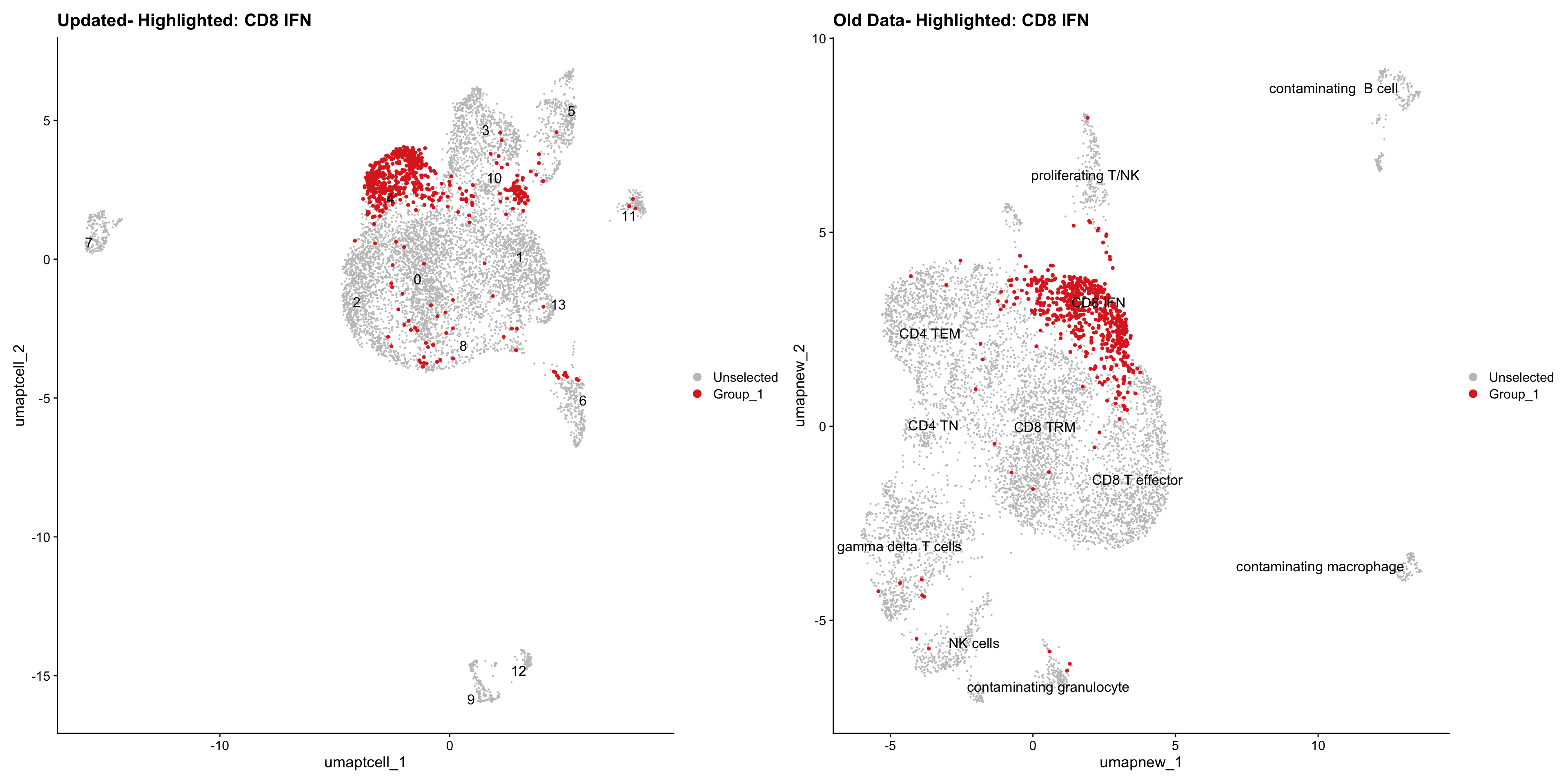
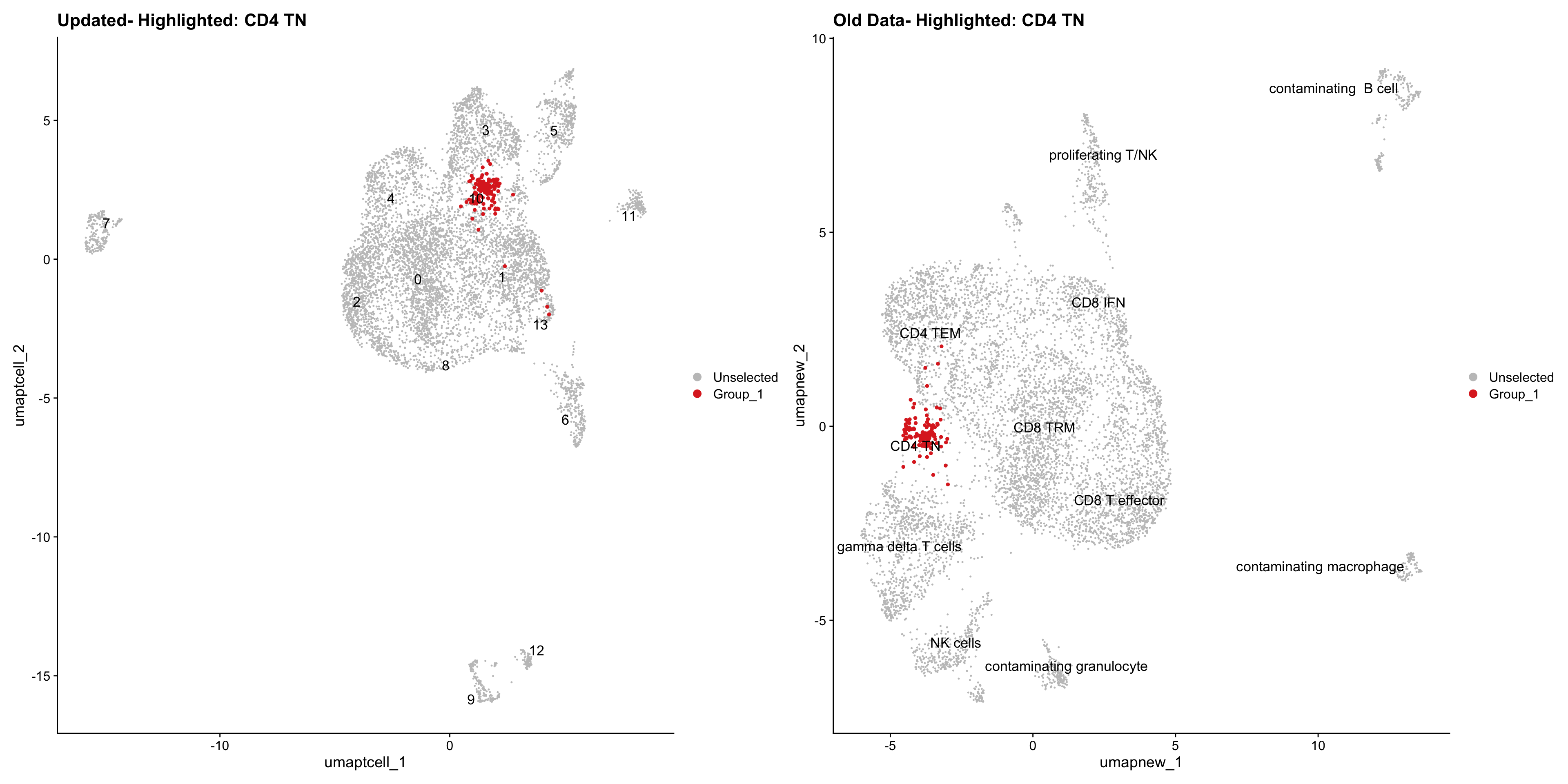
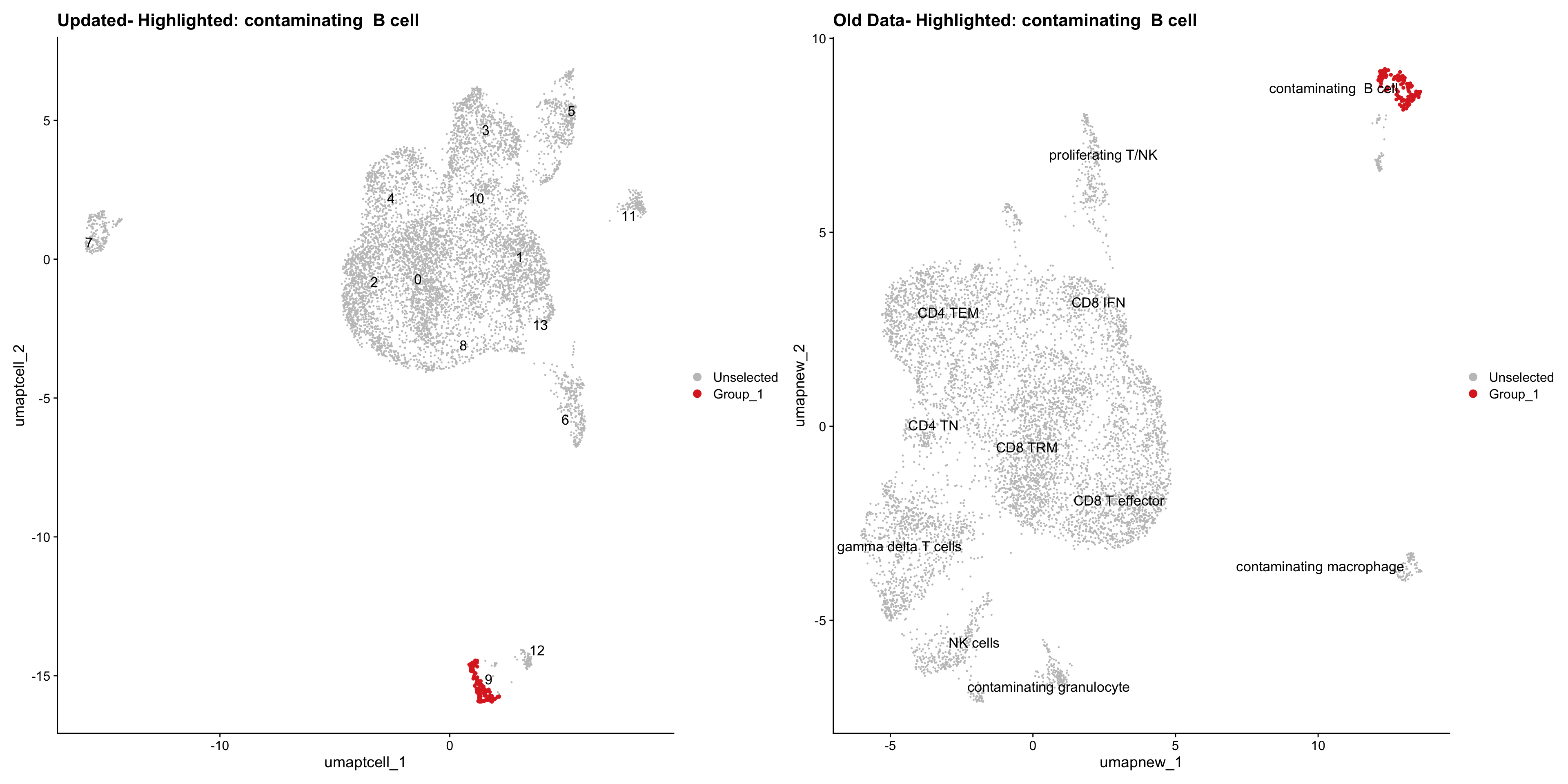
}Old data- cells from previous clusters higlighted
Loading old Subclustering seurat object of T cell population and comparing with the updated clustering.
out2 <- here("output",
"RDS", "AllBatches_Subclustering_SEUs", tissue,
paste0("G000231_Neeland_",tissue,".Tcell_population.subclusters.SEU.rds"))
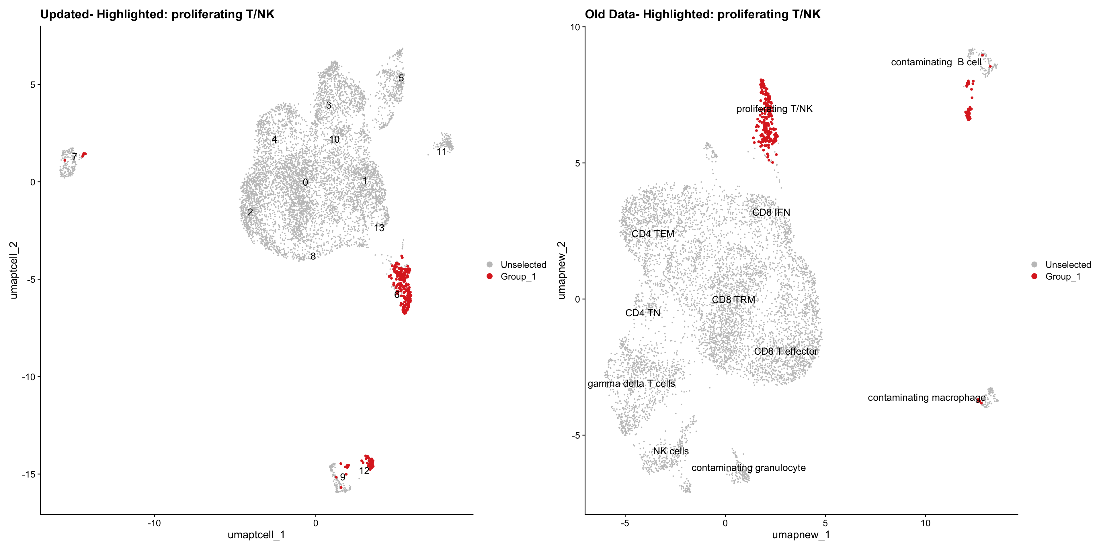
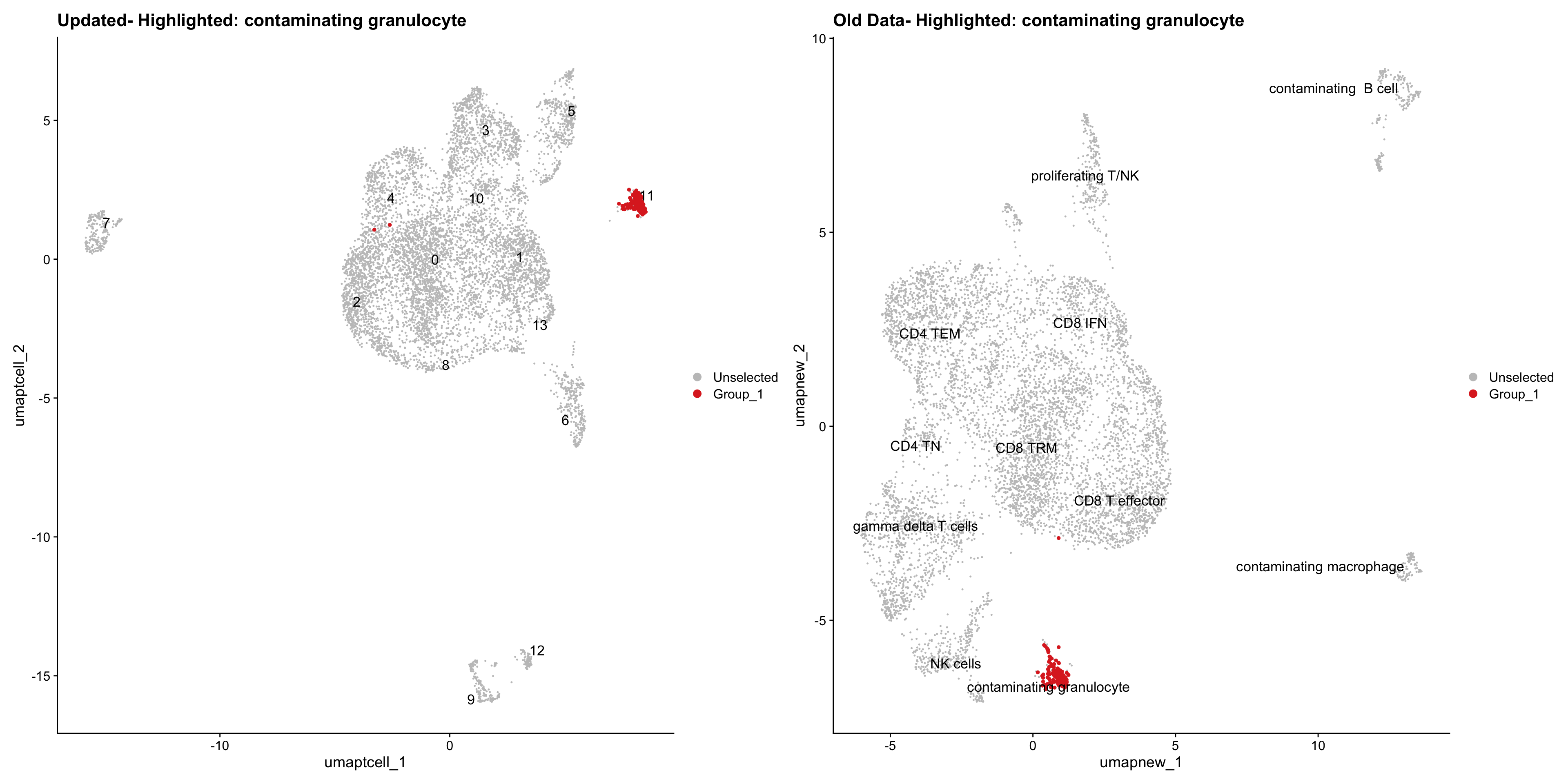
old_obj <- readRDS(out2)cell_types <- unique(old_obj$cell_labels_v2)
for (cell_type in cell_types) {
cl_cells <- WhichCells(old_obj, idents = cell_type)
p <- DimPlot(
paed_sub,
reduction = "umap.tcell",
label = TRUE,
label.size = 4.5,
repel = TRUE,
raster = FALSE,
cells.highlight = cl_cells
) +
ggtitle(paste("Updated- Highlighted:", cell_type))
p1 <- DimPlot(
old_obj,
reduction = "umap.new",
label = T,
label.size = 4.5,
repel = TRUE,
raster = FALSE,
cells.highlight = cl_cells
) +
ggtitle(paste("Old Data- Highlighted:", cell_type))
print(p | p1)
}
Summary Plots
palette1 <- paletteer::paletteer_d("ggthemes::Classic_20")
palette2 <- paletteer::paletteer_d("Polychrome::light")
combined_palette <- unique(c(palette1, palette2))

labels <- c( "predicted.ann_level_1","predicted.ann_level_2", "predicted.ann_level_3", "predicted.ann_level_4", "predicted.ann_level_5","predicted.ann_finest_level", "RNA_snn_res.0.5")

p <- vector("list",length(labels))
for(label in labels){
  paed_sub@meta.data %>%
    ggplot(aes(x = !!sym(label),
               fill = !!sym(label))) +
    geom_bar() +
    geom_text(aes(label = ..count..), stat = "count",
              vjust = -0.5, colour = "black", size = 2) +
    scale_y_log10() +
    theme(axis.text.x = element_blank(),
          axis.title.x = element_blank(),
          axis.ticks.x = element_blank()) +
    NoLegend() +
    labs(y = "No. Cells (log scale)") -> p1

  paed_sub@meta.data %>%
    dplyr::select(!!sym(label), donor_id) %>%
    group_by(!!sym(label), donor_id) %>%
    summarise(num = n()) %>%
    mutate(prop = num / sum(num)) %>%
  ggplot(aes(x = !!sym(label), y = prop * 100,
             fill = donor_id)) +
    geom_bar(stat = "identity") +
    theme(axis.text.x = element_text(angle = 90,
                                     vjust = 0.5,
                                     hjust = 1,
                                     size = 8)) +
    labs(y = "% Cells", fill = "Sample") +
  scale_fill_manual(values = combined_palette) -> p2

  (p1 / p2) & theme(legend.text = element_text(size = 8),
                  legend.key.size = unit(3, "mm")) -> p[[label]]
}
`summarise()` has grouped output by 'predicted.ann_level_1'. You can override
using the `.groups` argument.
`summarise()` has grouped output by 'predicted.ann_level_2'. You can override
using the `.groups` argument.
`summarise()` has grouped output by 'predicted.ann_level_3'. You can override
using the `.groups` argument.
`summarise()` has grouped output by 'predicted.ann_level_4'. You can override
using the `.groups` argument.
`summarise()` has grouped output by 'predicted.ann_level_5'. You can override
using the `.groups` argument.
`summarise()` has grouped output by 'predicted.ann_finest_level'. You can
override using the `.groups` argument.
`summarise()` has grouped output by 'RNA_snn_res.0.5'. You can override using
the `.groups` argument.p[[1]]
NULL
[[2]]
NULL
[[3]]
NULL
[[4]]
NULL
[[5]]
NULL
[[6]]
NULL
[[7]]
NULL
$predicted.ann_level_1Warning: The dot-dot notation (`..count..`) was deprecated in ggplot2 3.4.0.
ℹ Please use `after_stat(count)` instead.
This warning is displayed once every 8 hours.
Call `lifecycle::last_lifecycle_warnings()` to see where this warning was
generated.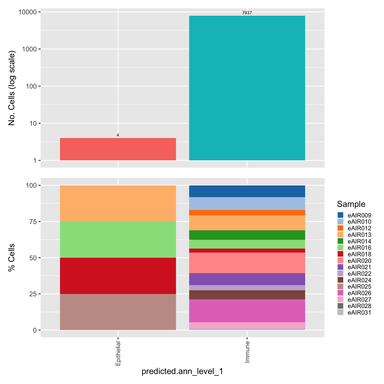
| Version | Author | Date |
|---|---|---|
| 3595ad0 | Gunjan Dixit | 2025-01-07 |
$predicted.ann_level_2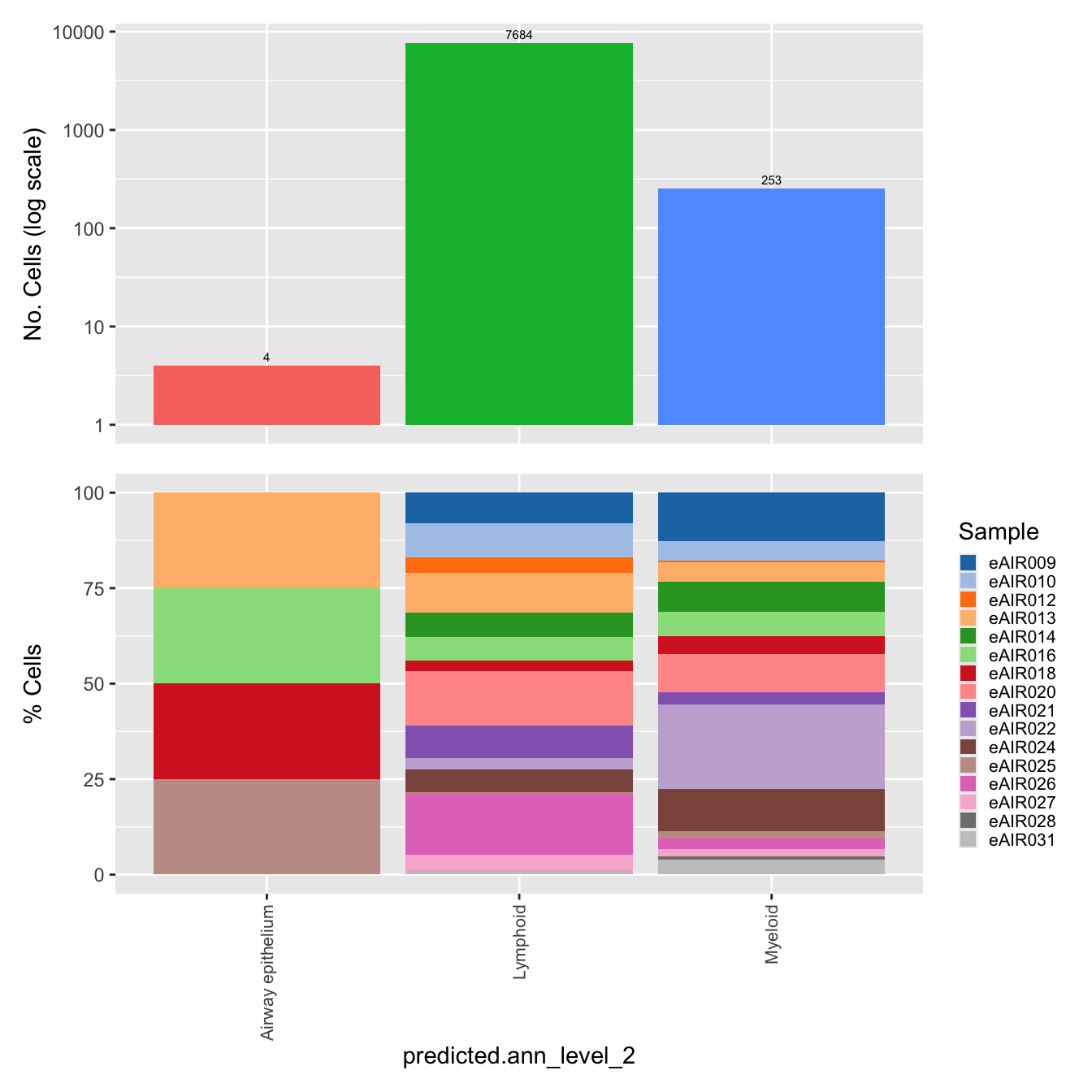
| Version | Author | Date |
|---|---|---|
| 3595ad0 | Gunjan Dixit | 2025-01-07 |
$predicted.ann_level_3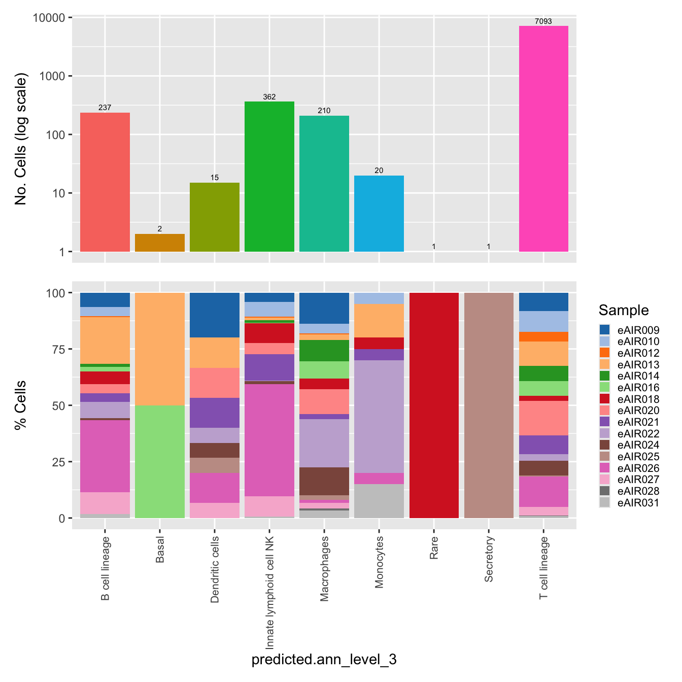
| Version | Author | Date |
|---|---|---|
| 3595ad0 | Gunjan Dixit | 2025-01-07 |
$predicted.ann_level_4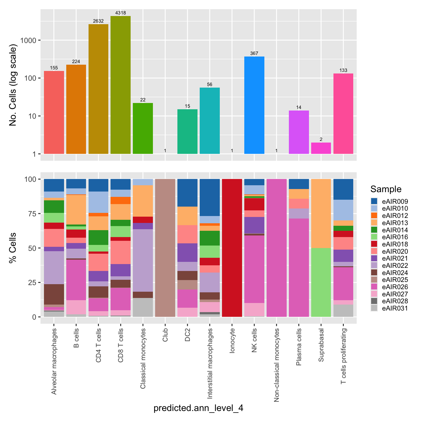
| Version | Author | Date |
|---|---|---|
| 3595ad0 | Gunjan Dixit | 2025-01-07 |
$predicted.ann_level_5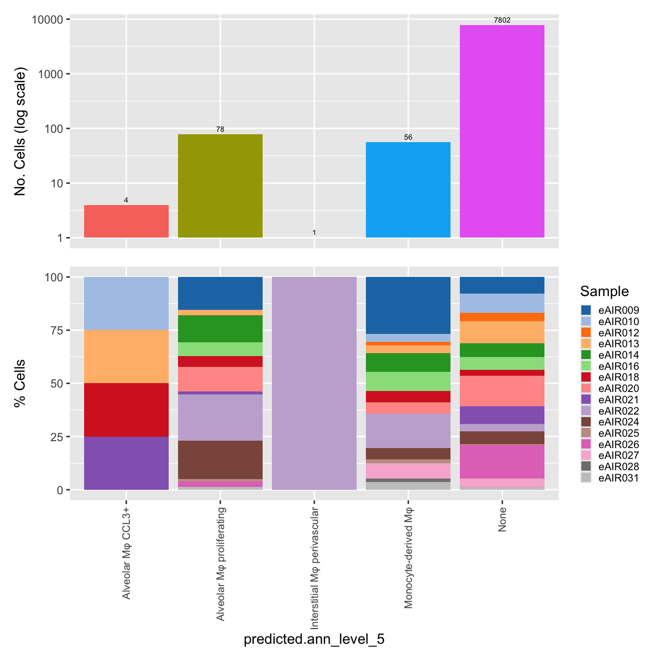
| Version | Author | Date |
|---|---|---|
| 3595ad0 | Gunjan Dixit | 2025-01-07 |
$predicted.ann_finest_level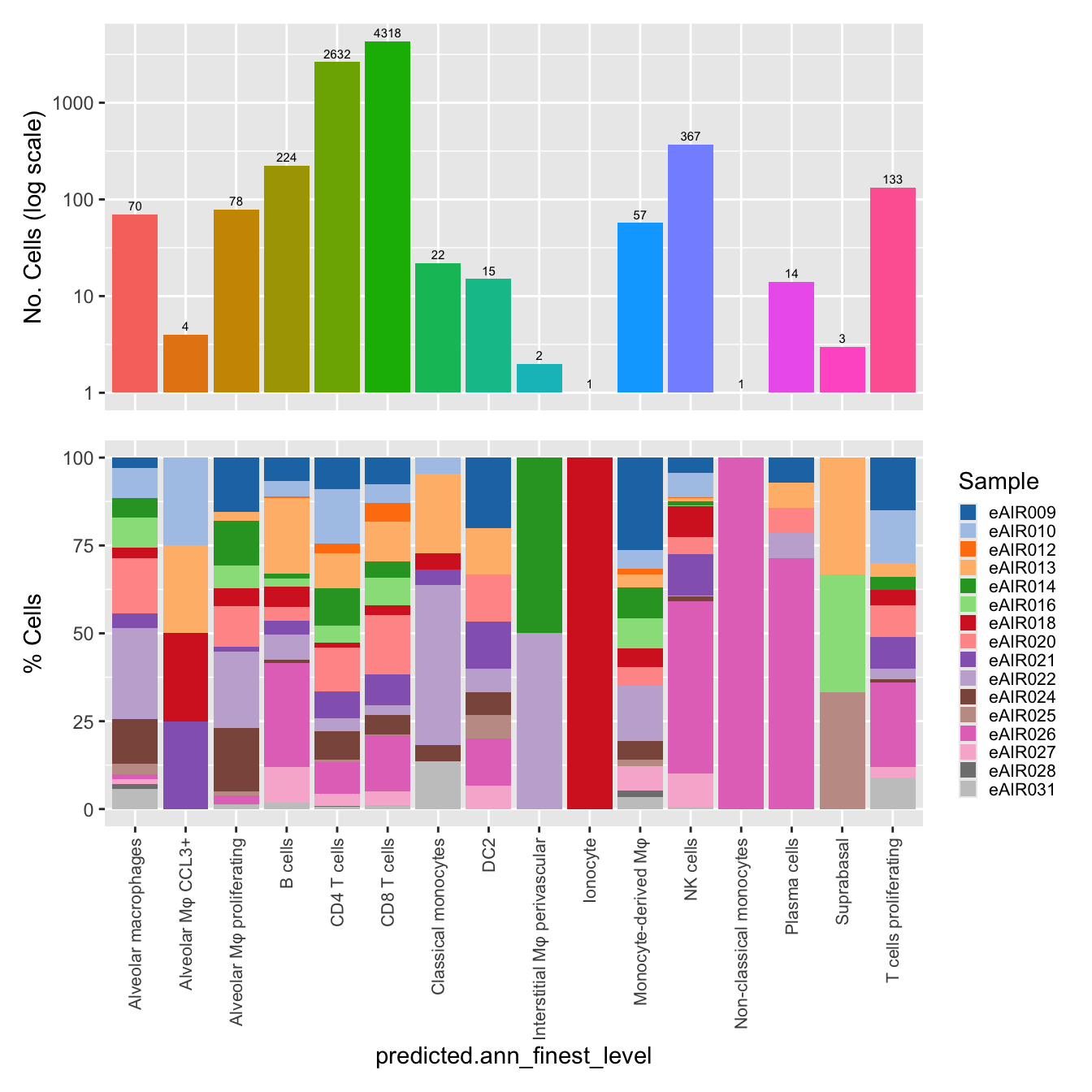
| Version | Author | Date |
|---|---|---|
| 3595ad0 | Gunjan Dixit | 2025-01-07 |
$RNA_snn_res.0.5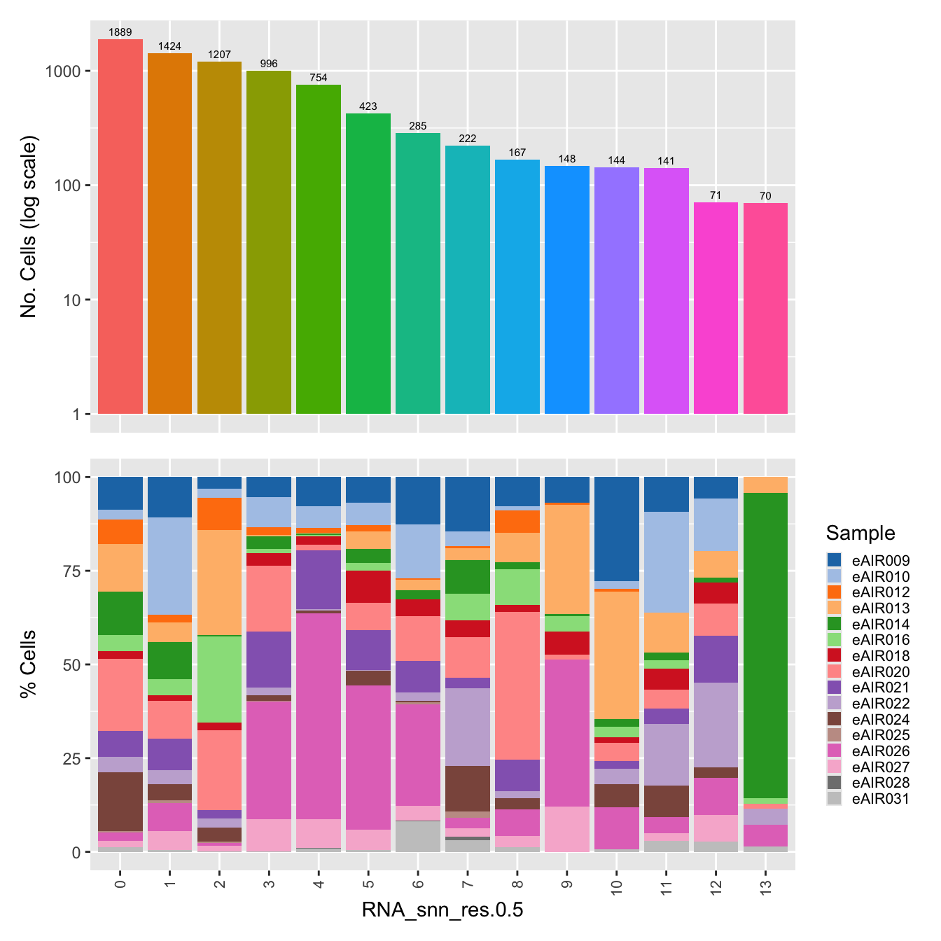
| Version | Author | Date |
|---|---|---|
| 3595ad0 | Gunjan Dixit | 2025-01-07 |
p1 <- paed_sub@meta.data %>%
     dplyr::select(!!sym(opt_res), cell_labels_v2) %>% ggplot(aes(x = !!sym(opt_res),
                                                                  fill = cell_labels_v2)) +
     geom_bar() +
     geom_text(aes(label = ..count..), stat = "count",
               vjust = -0.5, colour = "black", size = 2) +
     scale_y_log10() +
     theme(axis.text.x = element_blank(),
           axis.title.x = element_blank(),
           axis.ticks.x = element_blank()) +
     labs(y = "No. Cells (log scale)")

p2 <- paed_sub@meta.data %>%
  dplyr::select(!!sym(opt_res), Sample) %>%
  group_by(!!sym(opt_res), Sample) %>%
  summarise(num = n()) %>%
  mutate(prop = num / sum(num)) %>%
  ggplot(aes(x = !!sym(opt_res), y = prop * 100,
             fill = Sample)) +
  geom_bar(stat = "identity") +
  theme(axis.text.x = element_text(angle = 90,
                                   vjust = 0.5,
                                   hjust = 1,
                                   size = 8)) +
  labs(y = "% Cells", fill = "Sample") +
  scale_fill_manual(values = combined_palette)


# Combine the plots
(p1 / p2) & theme( legend.text = element_text(size = 8),
                            legend.key.size = unit(3, "mm"))
Save subclustered SEU object
out2 <- here("output",
            "RDS", "AllBatches_Subclustering_SEUs_v2", tissue,
             paste0("G000231_Neeland_",tissue,".Tcell_population.subclusters.SEU.rds"))
#dir.create(out2)
#if (!file.exists(out2)) {
  saveRDS(paed_sub, file = out2)
#}
Updated cell-type labels (T cell clusters)
cell_labels <- readxl::read_excel(here("data/cell_labels_Mel_v4_Dec2024/earlyAIR_BB_all.xlsx"), sheet = "T-reclustering")

new_cluster_names <- cell_labels %>%
  dplyr::select(cluster, annotation) %>%
  deframe()

paed_sub <- RenameIdents(paed_sub, new_cluster_names)
paed_sub@meta.data$cell_labels_v2 <- Idents(paed_sub)

p3 <- DimPlot(paed_sub, reduction = "umap.tcell", raster = FALSE, repel = TRUE, label = TRUE, label.size = 3.5) + ggtitle(paste0(tissue, ": UMAP with Updated T cell population"))

p3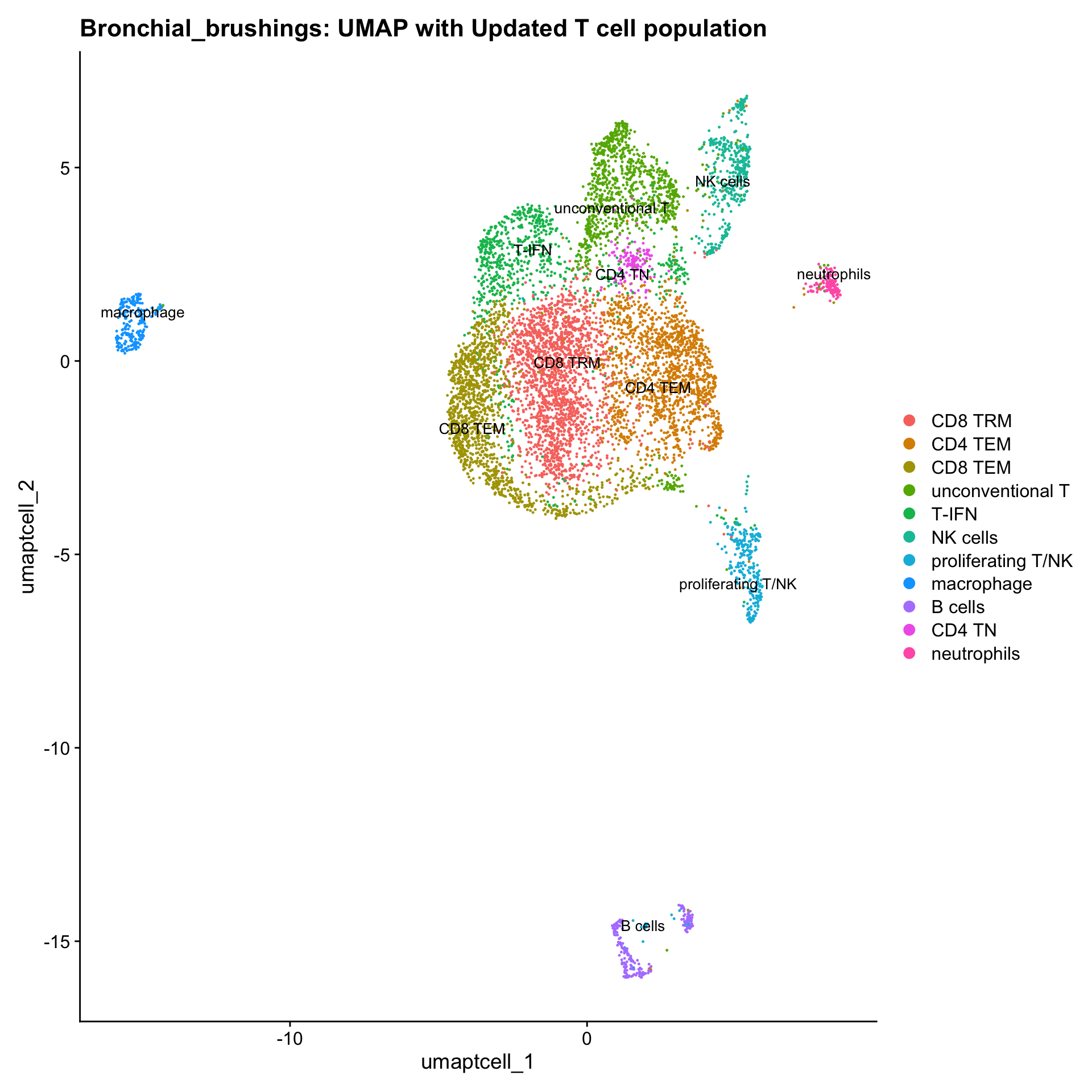
Save subclustered SEU object
out2 <- here("output",
            "RDS", "AllBatches_Annotated_Subclustering_SEUs_v2", tissue,
             paste0("G000231_Neeland_",tissue,".Tcell_population.subclusters.SEU.rds"))
#dir.create(out2)
if (!file.exists(out2)) {
  saveRDS(paed_sub, file = out2)
}
Reclustering B cells
The marker genes for this reclustering can be found here-
idx <- which(Idents(seu_obj) %in% "B cells for reclustering")
idx2 <- which(Idents(paed_sub) %in% "B cells")
paed_bcells <- merge(seu_obj[,idx], paed_sub[,idx2])
paed_bcells
An object of class Seurat
18046 features across 2987 samples within 1 assay
Active assay: RNA (18046 features, 2000 variable features)
6 layers present: counts.1, counts.2, data.1, scale.data.1, data.2, scale.data.2paed_bcells <- paed_bcells %>%
NormalizeData() %>%
FindVariableFeatures() %>%
ScaleData() %>%
RunPCA()Normalizing layer: counts.1Normalizing layer: counts.2Finding variable features for layer counts.1Finding variable features for layer counts.2Centering and scaling data matrixPC_ 1
Positive: TCL1A, DTX1, MARCKSL1, MEF2B, HMCES, P2RX5, SEMA4A, NUGGC, MYBL1, BCL7A
AFF2, ELL3, ASB13, MME, NEIL1, NIBAN3, A4GALT, BCL6, DCAF12, RAPGEF5
SLC2A5, MYBL2, CD38, IGHM, MKI67, BACH2, HIST1H1B, GSTP1, SPRED2, GCSAM
Negative: ITGAX, FCRL4, CAPG, TNFRSF13B, BHLHE40, IFI30, KCTD12, PREX1, VIM, GSN
SEMA7A, MPEG1, DUSP4, PTPN1, HCK, ADGRE5, MYO1F, CCR1, PLD4, FCRL5
ZBTB32, ZEB2, IL2RB, CCDC50, ITGB7, FLNA, CCR5, TESC, BHLHE41, ENTPD1
PC_ 2
Positive: FCMR, KLF2, CXCR4, IGHD, VPS37B, CD83, TSC22D3, IGHM, ZFP36L2, CD72
TMEM140, TENT5C, JUND, S1PR1, CD44, BCL2, SKI, PLAC8, TRIM22, PNPLA7
IQSEC1, IRF7, MMP17, SATB1, CCR7, CD69, NIBAN3, KDM6B, GRASP, HAPLN3
Negative: MKI67, KIFC1, HIST1H1B, TYMS, UHRF1, TK1, TOP2A, CDK1, HMGB2, RRM2
STMN1, BIRC5, BUB1, CDT1, HIST1H2BH, E2F2, E2F1, MYBL2, MCM4, HJURP
CCNB2, NCAPG, CDCA8, HIST1H4C, SHCBP1, CDC45, SPC25, MEF2B, CDC20, RGS13
PC_ 3
Positive: KDM6B, NR4A3, NFKBID, NR4A1, FOSL2, DUSP4, NR4A2, PIM3, EGR3, DUSP2
JUND, CD83, PER1, FOSB, SQSTM1, ADGRE5, GRASP, METRNL, NINJ1, G0S2
LMNA, NAB2, JUNB, SRGN, TRAF4, SLC7A5, TMEM88, EGR2, TRAF1, SLCO4A1
Negative: SAMD9L, STAT1, XAF1, IFI44L, SIGLEC14, IFI6, IFI44, TRIM22, PLAC8, EIF2AK2
OAS2, TNFSF10, OAS1, PARP14, ARHGAP15, IFIT3, IFIT1, MX1, APOL6, SP110
CMPK2, EPSTI1, SLFN5, TLR10, USP18, XRN1, RSAD2, IFIT2, RNF213, ZBP1
PC_ 4
Positive: TMSB4X, LTB, CD52, CXCR4, IL16, FCRL1, BANK1, FCRL2, TLR10, TCL1A
SPIB, SMIM14, SUN2, SNX22, HHEX, TSPAN33, NIBAN3, COTL1, PTPN6, MARCKSL1
CD72, SESN3, ELL3, CCR6, DTX1, MPEG1, PLEKHO1, ARHGAP15, FCMR, MS4A7
Negative: JCHAIN, CHPF, XBP1, MZB1, TXNDC5, FNDC3B, AQP3, DERL3, PRDM1, CKAP4
ERN1, FKBP11, SSR4, ITM2C, HID1, SDF2L1, HSP90B1, CRELD2, DUSP5, HYOU1
SEC11C, HM13, RRBP1, MANF, MAN1A1, NT5DC2, SELENOS, HPGD, TENT5C, WFS1
PC_ 5
Positive: JCHAIN, CHPF, DERL3, IGHA1, HSP90B1, TNFRSF17, MGAT4A, CD27, CD180, METTL7A
RHOQ, FCRL2, HID1, AQP3, CKAP4, SEC11C, IFNGR1, FCRL4, MS4A7, PDCD4
NXPE3, IGHA2, EVI2B, PLPP5, GALNT1, FNDC3B, DNAJB9, TLR10, LGALS1, ERN1
Negative: ISG15, OAS3, IFI6, CMPK2, IFIT1, IRF7, APOL6, LY6E, USP18, ISG20
MX1, RSAD2, MX2, TRIM22, IFIT2, XAF1, IFI44L, GBP1, IFIT3, UBE2L6
HAPLN3, OAS2, WARS, IFI44, SOCS1, HELZ2, STAT1, GBP4, EPSTI1, TNFSF10 paed_bcells <- RunUMAP(paed_bcells, dims = 1:30, reduction = "pca", reduction.name = "umap.bcell")09:10:20 UMAP embedding parameters a = 0.9922 b = 1.112Found more than one class "dist" in cache; using the first, from namespace 'spam'Also defined by 'BiocGenerics'09:10:20 Read 2987 rows and found 30 numeric columns09:10:20 Using Annoy for neighbor search, n_neighbors = 30Found more than one class "dist" in cache; using the first, from namespace 'spam'Also defined by 'BiocGenerics'09:10:20 Building Annoy index with metric = cosine, n_trees = 500% 10 20 30 40 50 60 70 80 90 100%[----|----|----|----|----|----|----|----|----|----|**************************************************|
09:10:20 Writing NN index file to temp file /var/folders/q8/kw1r78g12qn793xm7g0zvk94x2bh70/T//RtmphlxS57/file5dc1e32883c
09:10:20 Searching Annoy index using 1 thread, search_k = 3000
09:10:21 Annoy recall = 100%
09:10:21 Commencing smooth kNN distance calibration using 1 thread with target n_neighbors = 30
09:10:22 Initializing from normalized Laplacian + noise (using RSpectra)
09:10:22 Commencing optimization for 500 epochs, with 125160 positive edges
09:10:24 Optimization finishedmeta_data_columns <- colnames(paed_bcells@meta.data)
columns_to_remove <- grep("^RNA_snn_res", meta_data_columns, value = TRUE)
paed_bcells@meta.data <- paed_bcells@meta.data[, !(colnames(paed_bcells@meta.data) %in% columns_to_remove)]
resolutions <- seq(0.1, 1, by = 0.1)
paed_bcells <- FindNeighbors(paed_bcells, reduction = "pca", dims = 1:30)
paed_bcells <- FindClusters(paed_bcells, resolution = resolutions, algorithm = 3)Modularity Optimizer version 1.3.0 by Ludo Waltman and Nees Jan van Eck
Number of nodes: 2987
Number of edges: 109979
Running smart local moving algorithm...
Maximum modularity in 10 random starts: 0.9289
Number of communities: 3
Elapsed time: 1 seconds
Modularity Optimizer version 1.3.0 by Ludo Waltman and Nees Jan van Eck
Number of nodes: 2987
Number of edges: 109979
Running smart local moving algorithm...
Maximum modularity in 10 random starts: 0.8913
Number of communities: 6
Elapsed time: 0 seconds
Modularity Optimizer version 1.3.0 by Ludo Waltman and Nees Jan van Eck
Number of nodes: 2987
Number of edges: 109979
Running smart local moving algorithm...
Maximum modularity in 10 random starts: 0.8690
Number of communities: 9
Elapsed time: 0 seconds
Modularity Optimizer version 1.3.0 by Ludo Waltman and Nees Jan van Eck
Number of nodes: 2987
Number of edges: 109979
Running smart local moving algorithm...
Maximum modularity in 10 random starts: 0.8530
Number of communities: 11
Elapsed time: 0 seconds
Modularity Optimizer version 1.3.0 by Ludo Waltman and Nees Jan van Eck
Number of nodes: 2987
Number of edges: 109979
Running smart local moving algorithm...
Maximum modularity in 10 random starts: 0.8396
Number of communities: 11
Elapsed time: 0 seconds
Modularity Optimizer version 1.3.0 by Ludo Waltman and Nees Jan van Eck
Number of nodes: 2987
Number of edges: 109979
Running smart local moving algorithm...
Maximum modularity in 10 random starts: 0.8271
Number of communities: 11
Elapsed time: 0 seconds
Modularity Optimizer version 1.3.0 by Ludo Waltman and Nees Jan van Eck
Number of nodes: 2987
Number of edges: 109979
Running smart local moving algorithm...
Maximum modularity in 10 random starts: 0.8160
Number of communities: 12
Elapsed time: 0 seconds
Modularity Optimizer version 1.3.0 by Ludo Waltman and Nees Jan van Eck
Number of nodes: 2987
Number of edges: 109979
Running smart local moving algorithm...
Maximum modularity in 10 random starts: 0.8055
Number of communities: 12
Elapsed time: 0 seconds
Modularity Optimizer version 1.3.0 by Ludo Waltman and Nees Jan van Eck
Number of nodes: 2987
Number of edges: 109979
Running smart local moving algorithm...
Maximum modularity in 10 random starts: 0.7952
Number of communities: 13
Elapsed time: 0 seconds
Modularity Optimizer version 1.3.0 by Ludo Waltman and Nees Jan van Eck
Number of nodes: 2987
Number of edges: 109979
Running smart local moving algorithm...
Maximum modularity in 10 random starts: 0.7852
Number of communities: 13
Elapsed time: 0 secondsDimHeatmap(paed_bcells, dims = 1:10, cells = 500, balanced = TRUE)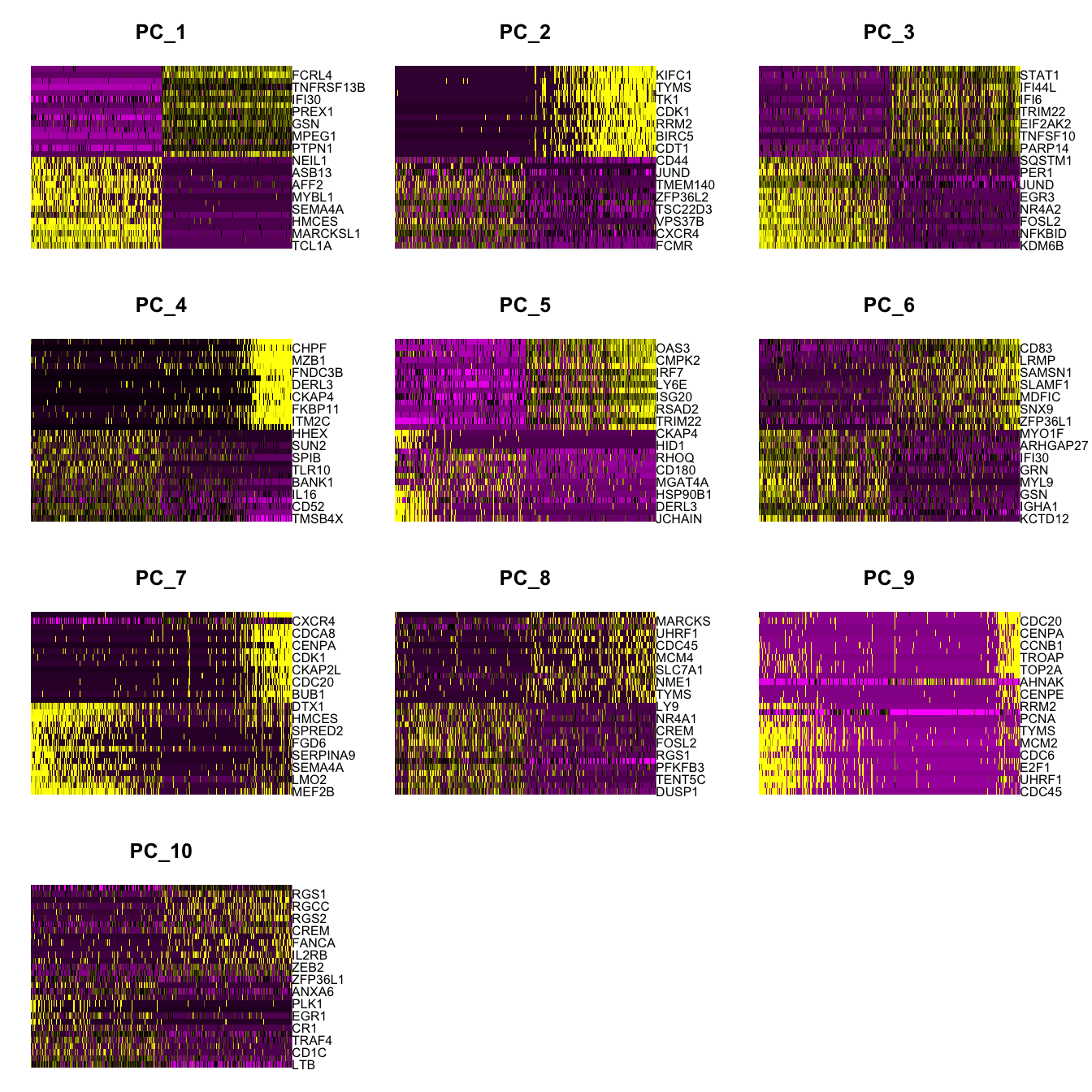
| Version | Author | Date |
|---|---|---|
| 3595ad0 | Gunjan Dixit | 2025-01-07 |
clustree(paed_bcells, prefix = "RNA_snn_res.")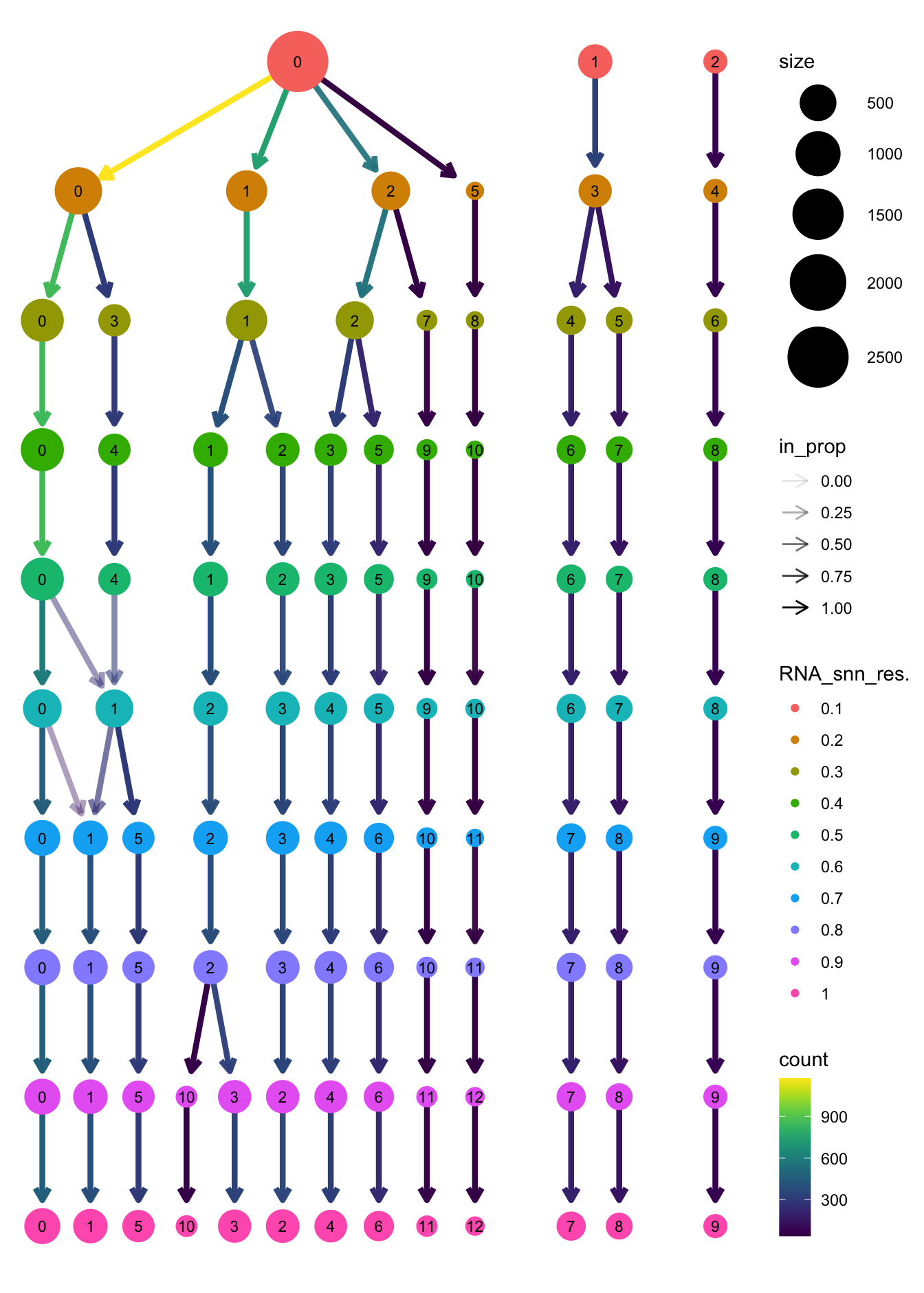
| Version | Author | Date |
|---|---|---|
| 3595ad0 | Gunjan Dixit | 2025-01-07 |
opt_res <- "RNA_snn_res.0.3"
n <- nlevels(paed_bcells$RNA_snn_res.0.3)
paed_bcells$RNA_snn_res.0.3 <- factor(paed_bcells$RNA_snn_res.0.3, levels = seq(0,n-1))
paed_bcells$seurat_clusters <- NULL
Idents(paed_bcells) <- paed_bcells$RNA_snn_res.0.3
DimPlot(paed_bcells, reduction = "umap.bcell", group.by = "RNA_snn_res.0.3", label = TRUE, label.size = 4.5, repel = TRUE, raster = FALSE )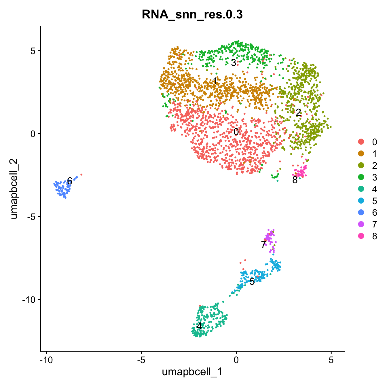
| Version | Author | Date |
|---|---|---|
| 3595ad0 | Gunjan Dixit | 2025-01-07 |
paed_bcells <- JoinLayers(paed_bcells)
paed_bcells.markers <- FindAllMarkers(paed_bcells, only.pos = TRUE, min.pct = 0.25, logfc.threshold = 0.25)
Calculating cluster 0Calculating cluster 1Calculating cluster 2Calculating cluster 3Calculating cluster 4Calculating cluster 5Calculating cluster 6Calculating cluster 7Calculating cluster 8paed_bcells.markers %>%
group_by(cluster) %>% unique() %>%
top_n(n = 5, wt = avg_log2FC) -> top5
paed_bcells.markers %>%
group_by(cluster) %>%
slice_head(n=1) %>%
pull(gene) -> best.wilcox.gene.per.cluster
best.wilcox.gene.per.cluster[1] "ADGRE5" "IGHD" "FCRL4" "MS4A1" "MEF2B" "MKI67" "CHPF" "PKMYT1"
[9] "FCAR" FeaturePlot(paed_bcells,features=best.wilcox.gene.per.cluster, reduction="umap.bcell",raster = FALSE, label = T, ncol = 3)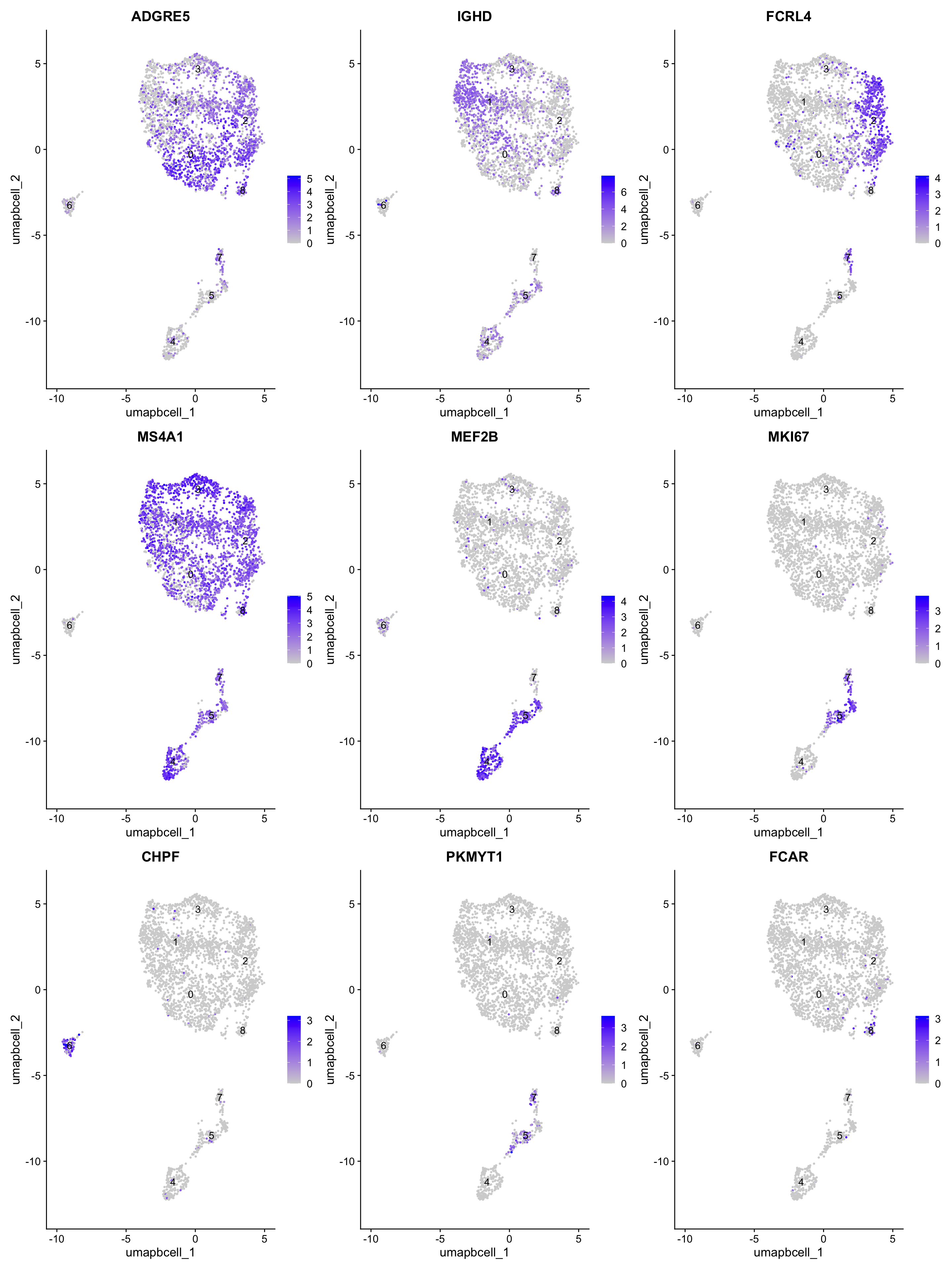
| Version | Author | Date |
|---|---|---|
| 3595ad0 | Gunjan Dixit | 2025-01-07 |
Top 10 marker genes from Seurat
## Seurat top markers
top10 <- paed_bcells.markers %>%
    group_by(cluster) %>%
    top_n(n = 10, wt = avg_log2FC) %>%
    ungroup() %>%
    distinct(gene, .keep_all = TRUE) %>%
    arrange(cluster, desc(avg_log2FC))

cluster_colors <- paletteer::paletteer_d("pals::glasbey")[factor(top10$cluster)]

DotPlot(paed_bcells,
        features = unique(top10$gene),
        group.by = opt_res,
        cols = c("azure1", "blueviolet"),
        dot.scale = 3, assay = "RNA") +
    RotatedAxis() +
    FontSize(y.text = 8, x.text = 12) +
    labs(y = element_blank(), x = element_blank()) +
    coord_flip() +
    theme(axis.text.y = element_text(color = cluster_colors)) +
    ggtitle("Top 10 marker genes per cluster (Seurat)")
Warning: Vectorized input to `element_text()` is not officially supported.
ℹ Results may be unexpected or may change in future versions of ggplot2.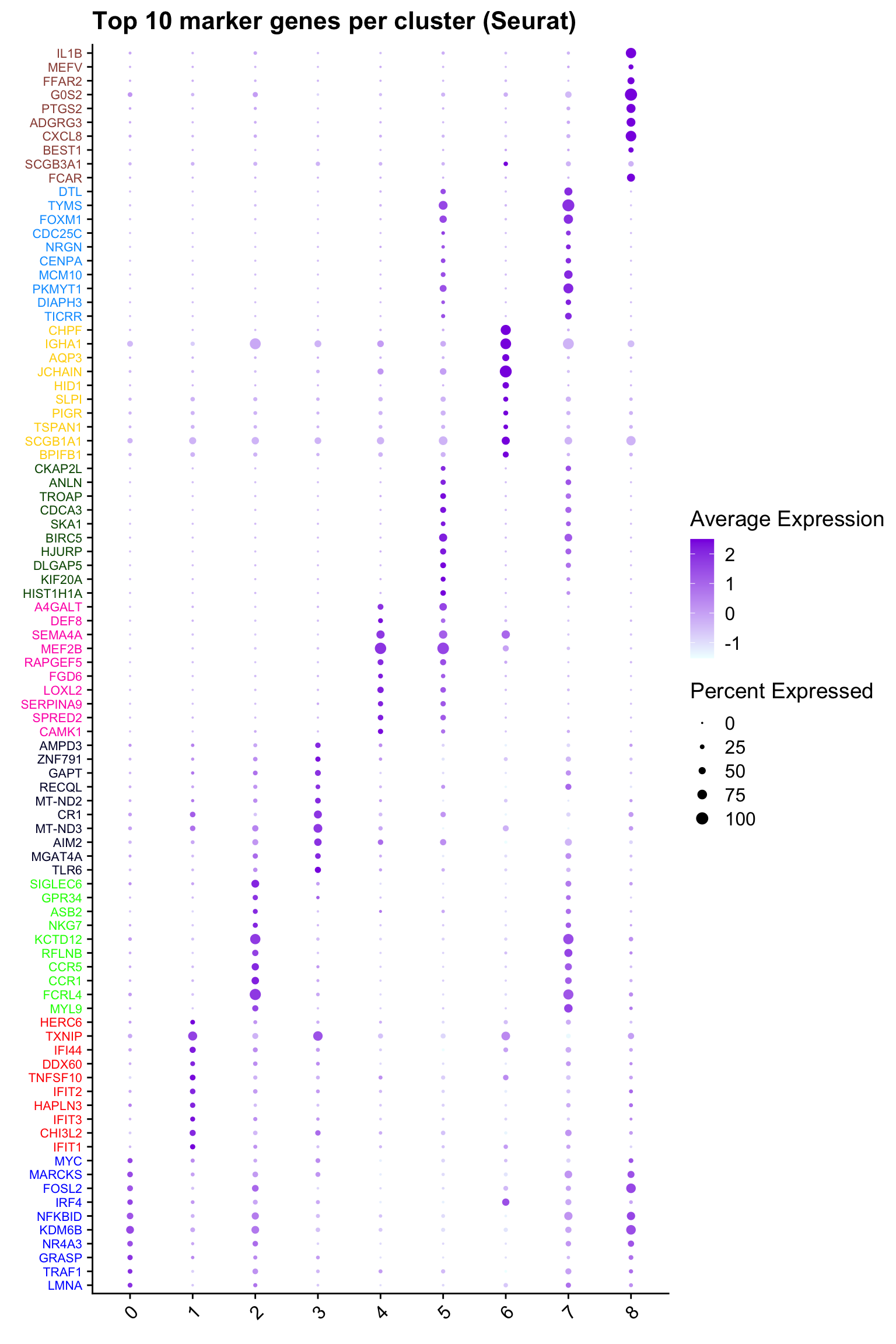
| Version | Author | Date |
|---|---|---|
| 3595ad0 | Gunjan Dixit | 2025-01-07 |
out_markers <- here("output",
"CSV_v2",tissue,
paste(tissue,"_Marker_genes_Reclustered_Bcell_population.",opt_res, sep = ""))
dir.create(out_markers, recursive = TRUE, showWarnings = FALSE)
for (cl in unique(paed_bcells.markers$cluster)) {
cluster_data <- paed_bcells.markers %>% dplyr::filter(cluster == cl)
file_name <- here(out_markers, paste0("G000231_Neeland_",tissue, "_cluster_", cl, ".csv"))
if (!file.exists(file_name)) {
write.csv(cluster_data, file = file_name)
}
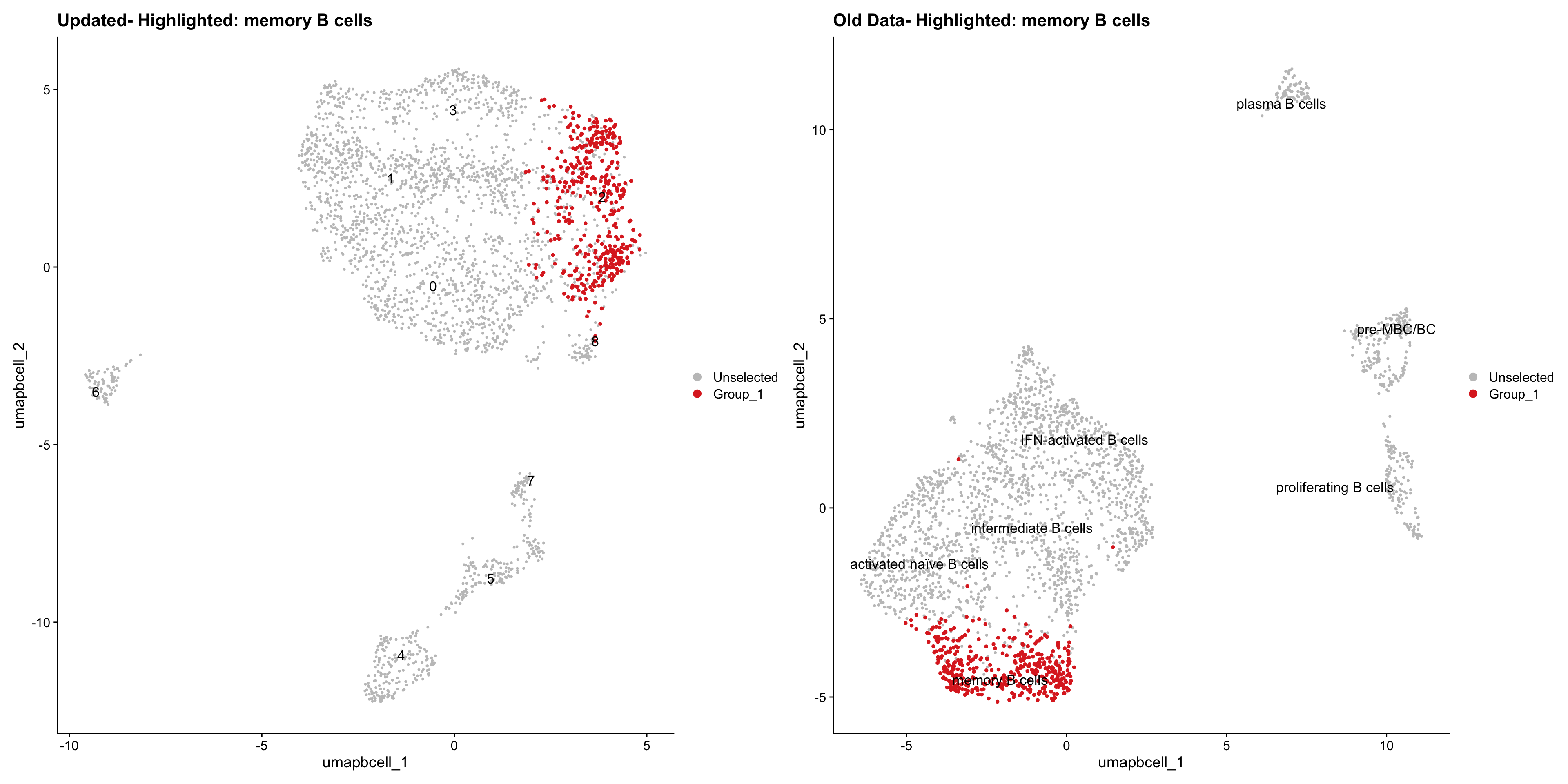
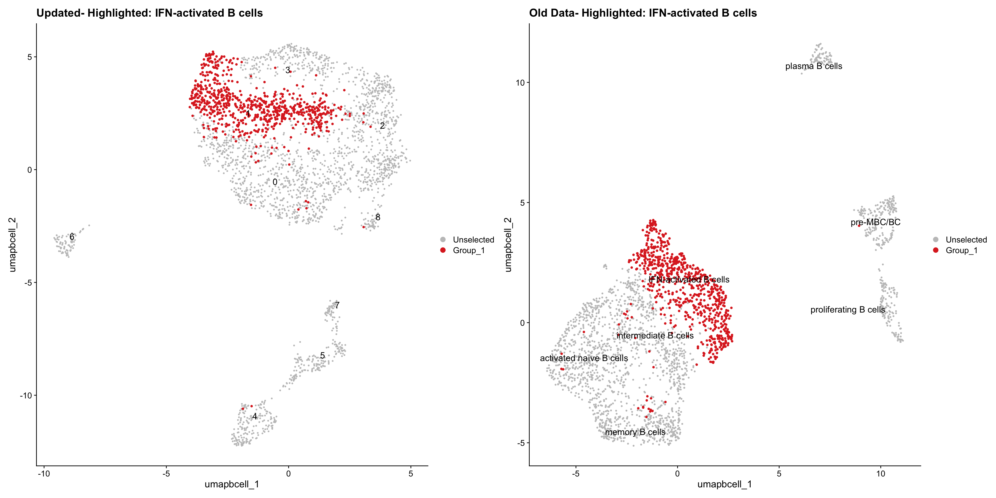
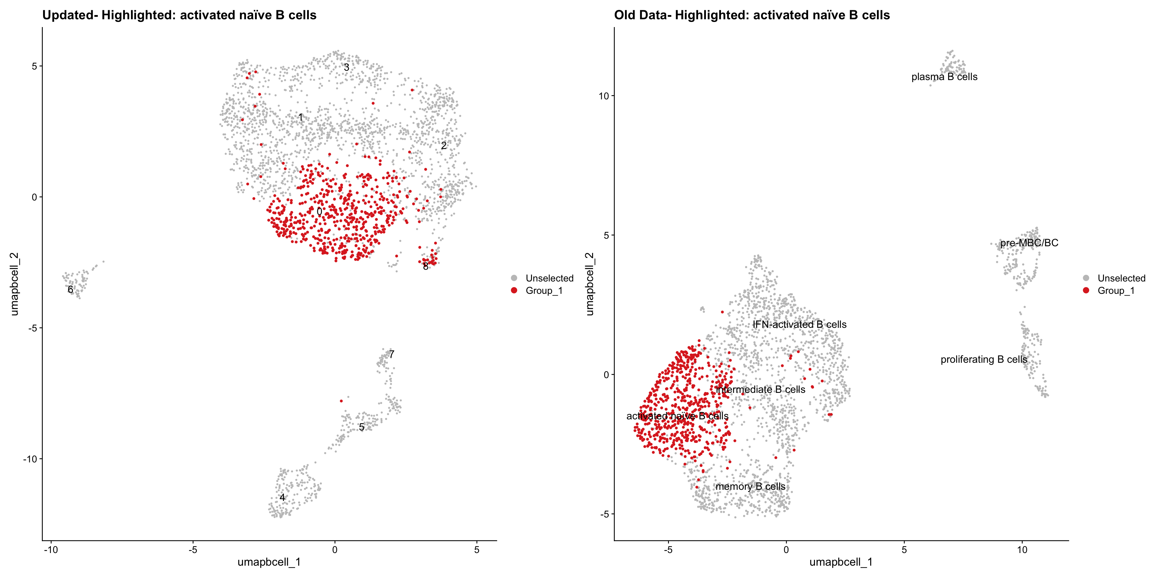
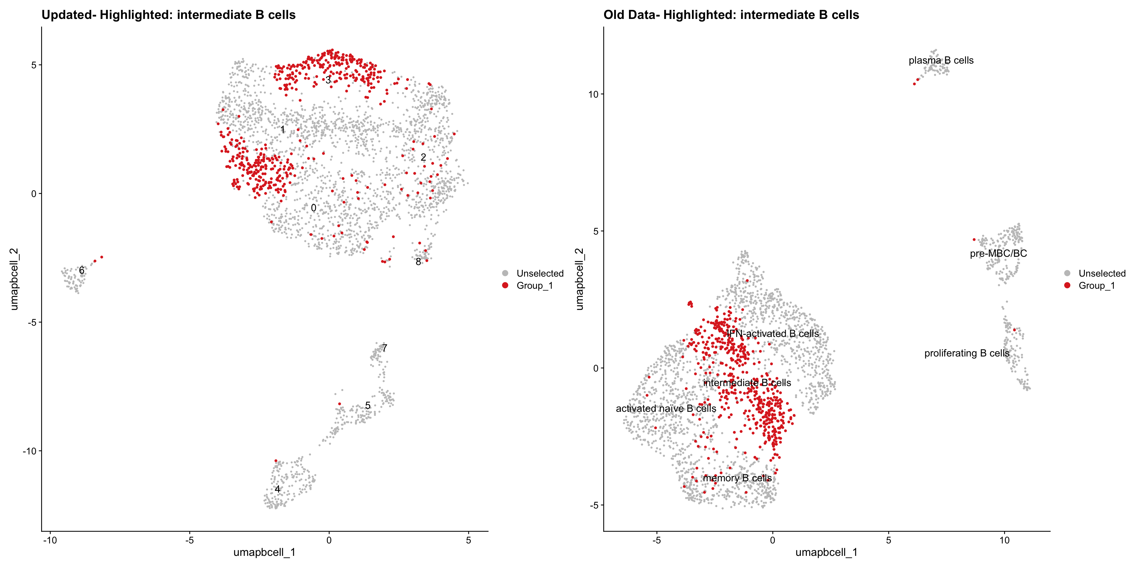
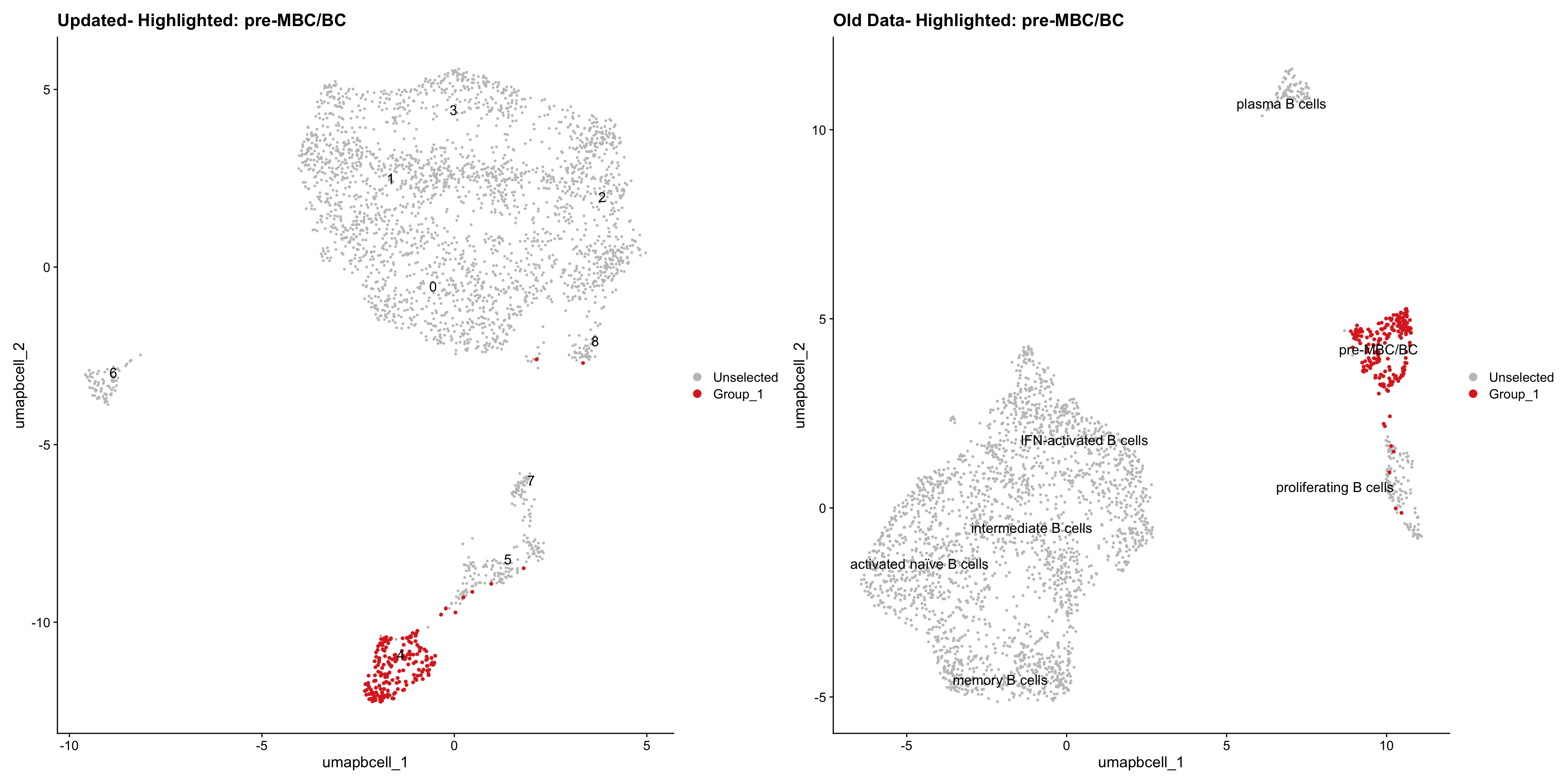
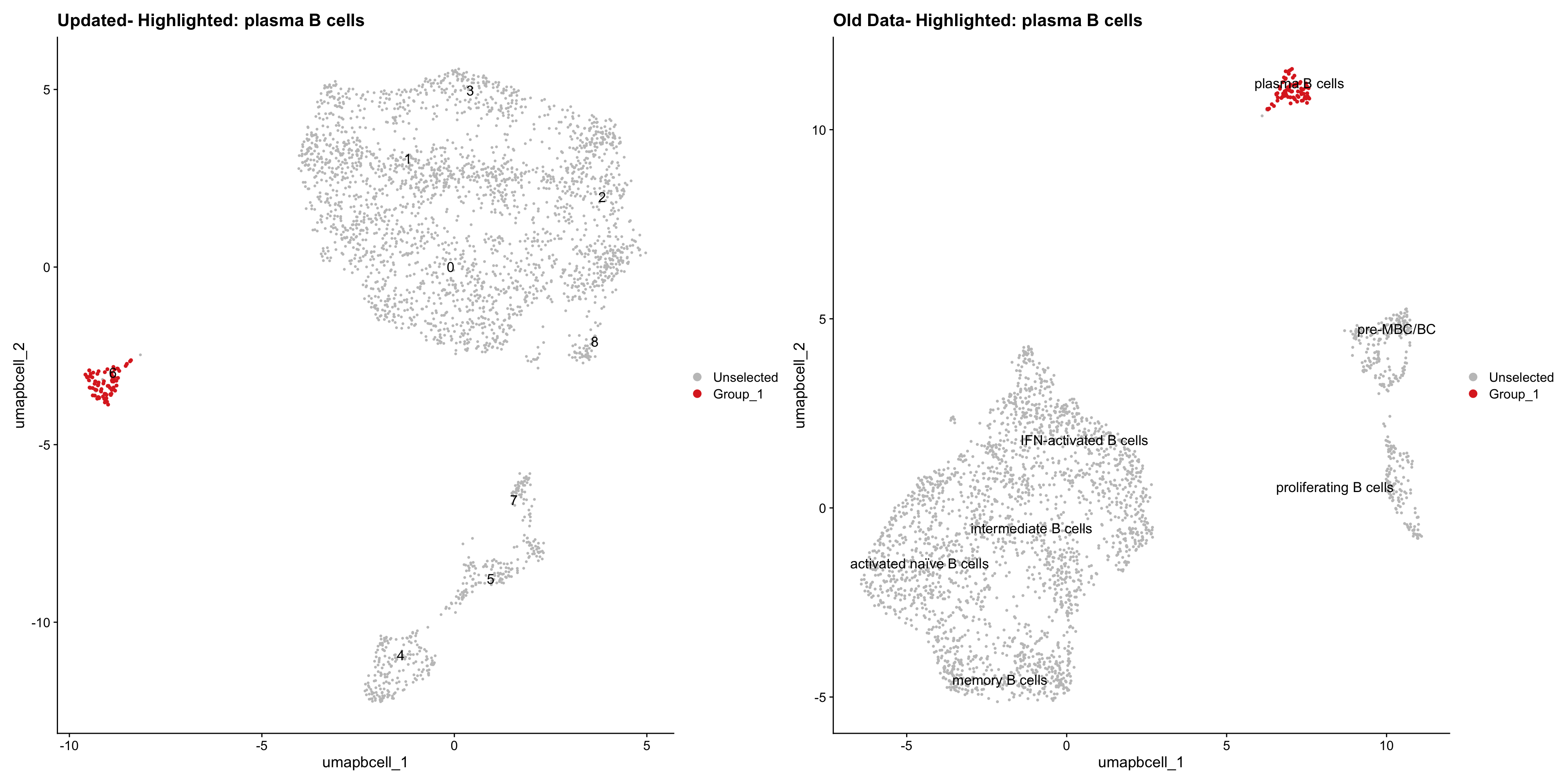
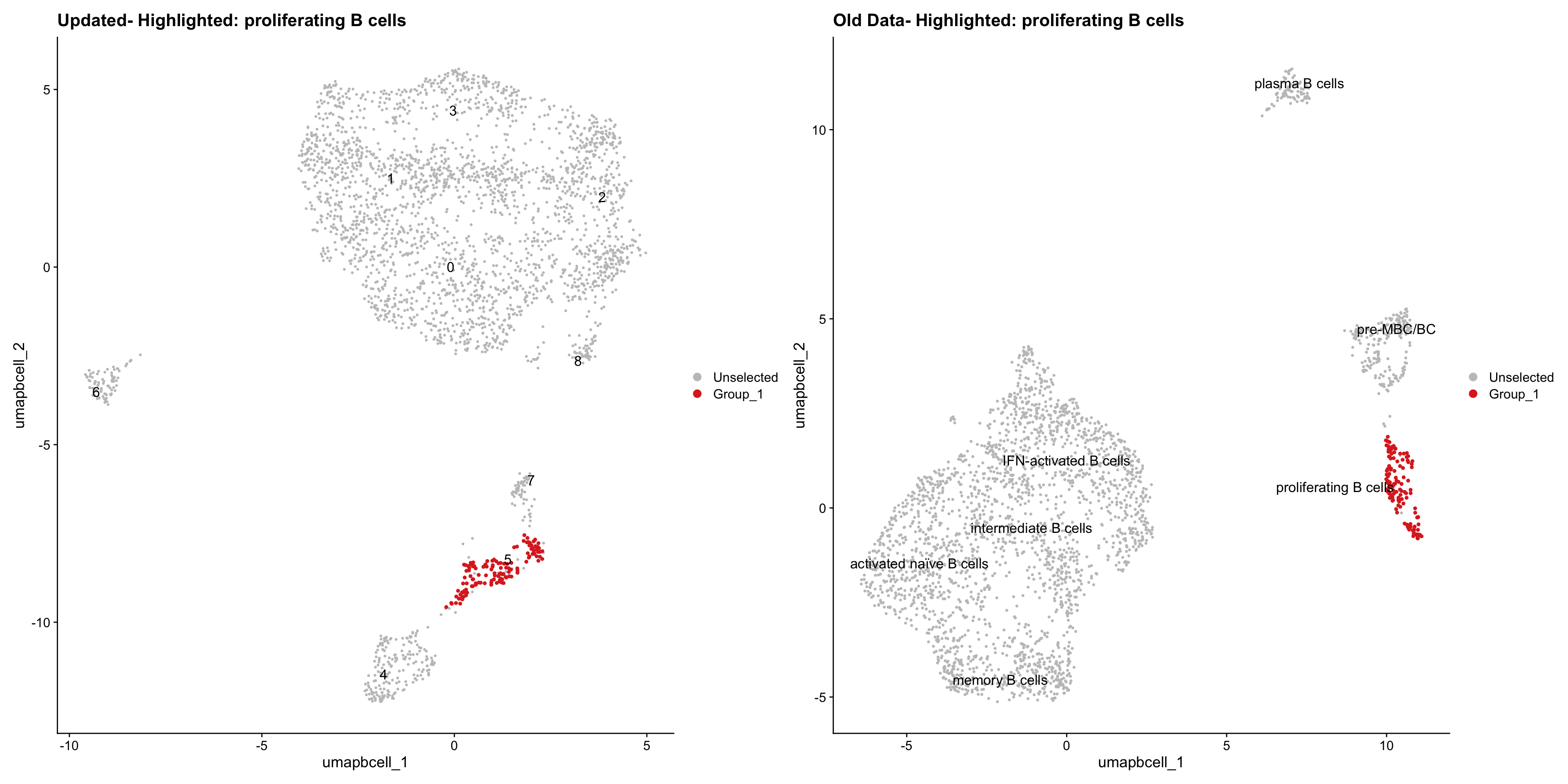
}Old data- cells from previous clusters higlighted
Loading old Subclustering seurat object of T cell population and comparing with the updated clustering.
out2 <- here("output",
            "RDS","AllBatches_Subclustering_SEUs", "AllBatches_Subclustering_v2_SEUs", tissue,
             paste0("G000231_Neeland_",tissue,".Bcell_population.subclusters.SEU.rds"))

old_obj <- readRDS(out2)
Idents(old_obj) <- old_obj$cell_labels_v3
cell_types <- unique(old_obj$cell_labels_v3)
for (cell_type in cell_types) {
cl_cells <- WhichCells(old_obj, idents = cell_type)
p <- DimPlot(
paed_bcells,
reduction = "umap.bcell",
label = TRUE,
label.size = 4.5,
repel = TRUE,
raster = FALSE,
cells.highlight = cl_cells
) +
ggtitle(paste("Updated- Highlighted:", cell_type))
p1 <- DimPlot(
old_obj,
reduction = "umap.bcell",
label = T,
label.size = 4.5,
repel = TRUE,
raster = FALSE,
cells.highlight = cl_cells
) +
ggtitle(paste("Old Data- Highlighted:", cell_type))
print(p | p1)
}
| Version | Author | Date |
|---|---|---|
| 3595ad0 | Gunjan Dixit | 2025-01-07 |
| Version | Author | Date |
|---|---|---|
| 3595ad0 | Gunjan Dixit | 2025-01-07 |
| Version | Author | Date |
|---|---|---|
| 3595ad0 | Gunjan Dixit | 2025-01-07 |
| Version | Author | Date |
|---|---|---|
| 3595ad0 | Gunjan Dixit | 2025-01-07 |
| Version | Author | Date |
|---|---|---|
| 3595ad0 | Gunjan Dixit | 2025-01-07 |
| Version | Author | Date |
|---|---|---|
| 3595ad0 | Gunjan Dixit | 2025-01-07 |
| Version | Author | Date |
|---|---|---|
| 3595ad0 | Gunjan Dixit | 2025-01-07 |
Updated cell-type labels (B cell clusters)
cell_labels <- readxl::read_excel(here("data/cell_labels_Mel_v4_Dec2024/earlyAIR_BB_all.xlsx"), sheet = "B-reclustering")

new_cluster_names <- cell_labels %>%
  dplyr::select(cluster, annotation) %>%
  deframe()

paed_bcells <- RenameIdents(paed_bcells, new_cluster_names)
paed_bcells@meta.data$cell_labels_v2 <- Idents(paed_bcells)

p3 <- DimPlot(paed_bcells, reduction = "umap.bcell", raster = FALSE, repel = TRUE, label = TRUE, label.size = 3.5) + ggtitle(paste0(tissue, ": UMAP with Updated B cell population"))

p3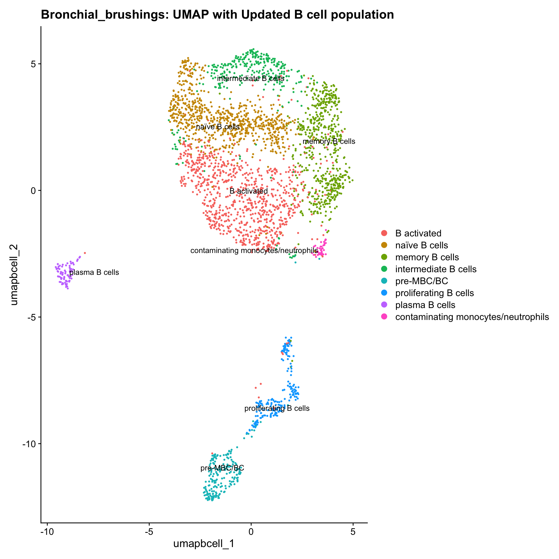
table(paed_bcells$cell_labels_v2)
                        B activated                       naïve B cells
                                858                                 747
                     memory B cells                intermediate B cells
                                567                                 303
                         pre-MBC/BC               proliferating B cells
                                201                                 188
                     plasma B cells contaminating monocytes/neutrophils
                                 84                                  39
Since there are only 39 contaminated monocytes/neutrophils here, I will chuck them out.
Excluding contaminating labels
idx <- which(grepl("^contaminating", Idents(paed_bcells)))
paed_bcells <- paed_bcells[, -idx]
Save subclustered SEU object Bcells
out2 <- here("output",
            "RDS", "AllBatches_Annotated_Subclustering_SEUs_v2", tissue,
             paste0("G000231_Neeland_",tissue,".Bcell_population.subclusters.SEU.rds"))
#dir.create(out2)
if (!file.exists(out2)) {
  saveRDS(paed_bcells, file = out2)
}
Other Clusters (excluding subclusters)
idx <- which(Idents(seu_obj) %in% c("T cells for reclustering", "B cells for reclustering"))
paed_other <- seu_obj[,-idx]
paed_other
An object of class Seurat
18046 features across 29637 samples within 1 assay
Active assay: RNA (18046 features, 2000 variable features)
3 layers present: counts, data, scale.data
2 dimensional reductions calculated: pca, umapSave subclustered SEU object ( All other cells)
paed_other$cell_labels_v2 <-paed_other$cell_labels
out2 <- here("output",
            "RDS", "AllBatches_Annotated_Subclustering_SEUs_v2", tissue,
             paste0("G000231_Neeland_",tissue,".all_other.subclusters.SEU.rds"))
#dir.create(out2)
if (!file.exists(out2)) {
  saveRDS(paed_other, file = out2)
}
Merge seurat objects of subclusters
files <- list.files(here("output",
            "RDS", "AllBatches_Annotated_Subclustering_SEUs_v2", tissue),
                    full.names = TRUE)

seuLst <- lapply(files, function(f) readRDS(f))

seu <- merge(seuLst[[1]],
             y = c(seuLst[[2]],
                   seuLst[[3]]))
Warning: Some cell names are duplicated across objects provided. Renaming to
enforce unique cell names.seuAn object of class Seurat
18046 features across 40526 samples within 1 assay
Active assay: RNA (18046 features, 2000 variable features)
13 layers present: counts.1, counts.1.2, counts.2.2, counts.3, data.1, scale.data.1, data.1.2, scale.data.1.2, data.2.2, scale.data.2.2, scale.data.2, data.3, scale.data.3levels(seu$cell_labels_v2)[levels(seu$cell_labels_v2) == "macrophage"] <- "macrophages"
levels(Idents(seu))[levels(Idents(seu)) == "macrophage"] <- "macrophages"
seu$cell_labels_v2 <- Idents(seu)merged <- seu %>%
NormalizeData() %>%
FindVariableFeatures() %>%
ScaleData() %>%
RunPCA()Normalizing layer: counts.1Normalizing layer: counts.1.2Normalizing layer: counts.2.2Normalizing layer: counts.3Finding variable features for layer counts.1Finding variable features for layer counts.1.2Finding variable features for layer counts.2.2Finding variable features for layer counts.3Centering and scaling data matrixPC_ 1
Positive: CD68, SERPINA1, LYZ, TYROBP, FCER1G, MS4A7, MARCO, C1QB, GRN, C1QA
LRP1, MSR1, C1QC, OLR1, CTSL, FTL, GPNMB, TIMP2, IFI30, EMILIN2
ADAMTSL4, SLC15A3, CYP27A1, FABP4, SPI1, SLC11A1, PSAP, LGALS1, CTSZ, GAA
Negative: ELF3, CD24, CLU, SLC34A2, TRAF4, DDIT4, FCGBP, ZMYND10, LBH, NUCB2
B9D1, LRP11, DHCR24, PPL, PRSS22, ATP8B1, C12orf75, PARD3, TNFAIP8L1, CX3CL1
MAPK8IP1, IL32, TRIB2, ASS1, TFF3, TNFSF10, CRIP2, CFB, WDR34, RRAD
PC_ 2
Positive: CXCR4, SRGN, TRBC2, IL2RB, LCP2, PLEKHO1, CD3E, TNFRSF1B, CCL5, CD69
ANXA6, CD7, CD3D, NKG7, PREX1, IL32, ADAM19, CD96, CD8A, SPOCK2
LTB, SERPINB9, ITGB7, ARL4C, GPR132, CXCR6, LCK, CCR5, ZAP70, PRF1
Negative: ALDH1A1, ELF3, PLXNB2, TSPAN3, SDC4, SLC34A2, CD9, DHCR24, LRP11, S100A6
AQP3, APP, DHRS3, ANXA2, IGFBP2, CTNNA1, CD24, TUBB4B, CFB, GSTP1
ST14, PDLIM1, CTNND1, CLU, LGALS3, C3, DHRS9, PPL, ANXA4, ATP8B1
PC_ 3
Positive: IDO1, SAT1, APOBEC3A, LILRB2, IFITM3, MEFV, SPHK1, C15orf48, CD300E, LILRA5
SOCS3, IER3, CXCL10, CXCL11, CSF3R, CALHM6, TIMP1, CDKN1A, ADGRE2, SERPINB9
WARS, IL1RN, SOD2, ISG15, IL4I1, NLRP3, NINJ1, VAMP5, MX2, GBP1
Negative: SPN, SCD, GCHFR, FABP4, MME, CRIP1, AMIGO2, BHLHE41, SLC47A1, CYP27A1
GPD1, PCOLCE2, ACO1, CES1, VSIG4, CPE, TRBC2, CD3D, LPL, APOC1
RBP4, AKR1B1, ADTRP, VAT1, C8B, CD3E, SPARC, MGST3, CCL5, CITED2
PC_ 4
Positive: CD7, CCL5, CD3E, IL32, CD3D, CD8A, CXCR6, PRF1, KLRK1, CD96
CD3G, ZAP70, GZMA, KLRD1, AHNAK, IL2RB, CTSW, PRKCH, GNLY, TRBC2
NKG7, MATK, LCP2, ID2, TIGIT, TNIK, CST7, LCK, CSF1, ANXA1
Negative: MYBL2, KIFC1, MKI67, CD79A, TYMS, AURKB, HIST1H1B, PAX5, POU2AF1, UHRF1
TOP2A, MS4A1, CD79B, TK1, SPIB, CD19, RRM2, FOXM1, ZWINT, BIRC5
ASF1B, TPX2, SPC24, CD22, IGKC, PKMYT1, CDK1, HIST1H2BH, E2F2, E2F1
PC_ 5
Positive: ZMYND10, B9D1, RRAD, SPACA9, DZIP1L, C22orf15, TNFAIP8L1, CFAP58, BASP1, TUBB4B
LZTFL1, RPGRIP1L, C12orf75, GSTA2, TUB, KCTD12, ERICH5, ANKRD37, ZMYND12, PKIG
MAP1B, IFT43, HSPH1, PLAAT2, DNAJA4, ZC2HC1A, LRP11, WDR34, CES4A, IGFBP2
Negative: GPRC5A, SDC1, A4GALT, CEACAM5, SLC6A14, EPAS1, ASS1, CXCL6, ID1, GCNT3
IGFBP3, SPDEF, S100P, UPK1B, LYPD2, PDZK1IP1, FHL2, VMO1, KRT17, ALPL
SDCBP2, CTSC, MSLN, CXCL1, TNC, C3, TCIM, PI3, MGST1, RHOC merged <- RunUMAP(merged, dims = 1:30, reduction = "pca", reduction.name = "umap.merged")09:11:25 UMAP embedding parameters a = 0.9922 b = 1.112Found more than one class "dist" in cache; using the first, from namespace 'spam'Also defined by 'BiocGenerics'09:11:25 Read 40526 rows and found 30 numeric columns09:11:25 Using Annoy for neighbor search, n_neighbors = 30Found more than one class "dist" in cache; using the first, from namespace 'spam'Also defined by 'BiocGenerics'09:11:25 Building Annoy index with metric = cosine, n_trees = 500% 10 20 30 40 50 60 70 80 90 100%[----|----|----|----|----|----|----|----|----|----|**************************************************|
09:11:27 Writing NN index file to temp file /var/folders/q8/kw1r78g12qn793xm7g0zvk94x2bh70/T//RtmphlxS57/file5dcfce996c
09:11:27 Searching Annoy index using 1 thread, search_k = 3000
09:11:34 Annoy recall = 100%
09:11:34 Commencing smooth kNN distance calibration using 1 thread with target n_neighbors = 30
09:11:35 Initializing from normalized Laplacian + noise (using RSpectra)
09:11:38 Commencing optimization for 200 epochs, with 1696976 positive edges
09:11:49 Optimization finishedp4 <- DimPlot(merged, reduction = "umap.merged", group.by = "cell_labels_v2",raster = FALSE, repel = TRUE, label = TRUE, label.size = 4.5) + ggtitle(paste0(tissue, ": UMAP with annotations")) + NoLegend()
p4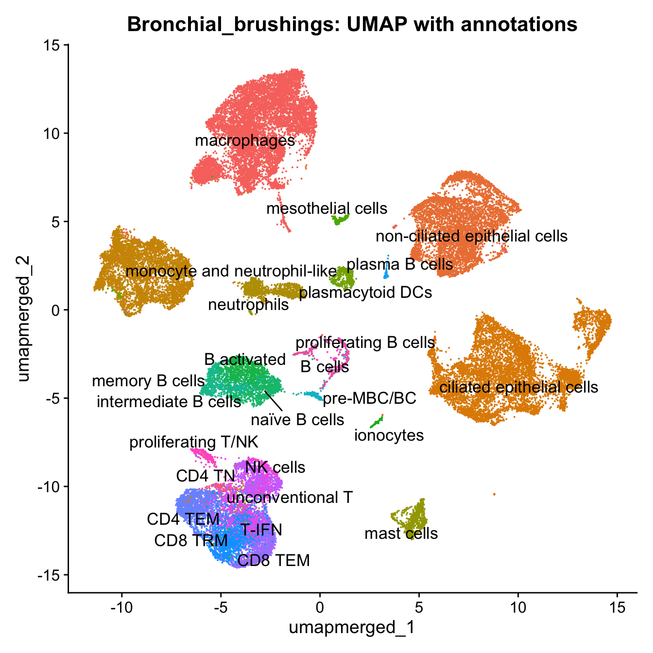
Save Final SEU object (All cells)
out3 <- here("output",
            "RDS", "AllBatches_Final_Clusters_SEUs_v2",
             paste0("G000231_Neeland_",tissue,".final_clusters.SEU.rds"))

if (!file.exists(out3)) {
  saveRDS(merged, file = out3)
}
Session Info
sessioninfo::session_info()─ Session info ───────────────────────────────────────────────────────────────
setting value
version R version 4.3.2 (2023-10-31)
os macOS 15.2
system aarch64, darwin20
ui X11
language (EN)
collate en_US.UTF-8
ctype en_US.UTF-8
tz Australia/Melbourne
date 2025-01-16
pandoc 3.1.1 @ /Users/dixitgunjan/Desktop/RStudio.app/Contents/Resources/app/quarto/bin/tools/ (via rmarkdown)
─ Packages ───────────────────────────────────────────────────────────────────
package * version date (UTC) lib source
abind 1.4-5 2016-07-21 [1] CRAN (R 4.3.0)
AnnotationDbi * 1.64.1 2023-11-02 [1] Bioconductor
backports 1.4.1 2021-12-13 [1] CRAN (R 4.3.0)
beeswarm 0.4.0 2021-06-01 [1] CRAN (R 4.3.0)
Biobase * 2.62.0 2023-10-26 [1] Bioconductor
BiocGenerics * 0.48.1 2023-11-02 [1] Bioconductor
BiocManager 1.30.22 2023-08-08 [1] CRAN (R 4.3.0)
BiocStyle * 2.30.0 2023-10-26 [1] Bioconductor
Biostrings 2.70.2 2024-01-30 [1] Bioconductor 3.18 (R 4.3.2)
bit 4.0.5 2022-11-15 [1] CRAN (R 4.3.0)
bit64 4.0.5 2020-08-30 [1] CRAN (R 4.3.0)
bitops 1.0-7 2021-04-24 [1] CRAN (R 4.3.0)
blob 1.2.4 2023-03-17 [1] CRAN (R 4.3.0)
bslib 0.6.1 2023-11-28 [1] CRAN (R 4.3.1)
cachem 1.0.8 2023-05-01 [1] CRAN (R 4.3.0)
callr 3.7.5 2024-02-19 [1] CRAN (R 4.3.1)
cellranger 1.1.0 2016-07-27 [1] CRAN (R 4.3.0)
checkmate 2.3.1 2023-12-04 [1] CRAN (R 4.3.1)
cli 3.6.2 2023-12-11 [1] CRAN (R 4.3.1)
cluster 2.1.6 2023-12-01 [1] CRAN (R 4.3.1)
clustree * 0.5.1 2023-11-05 [1] CRAN (R 4.3.1)
codetools 0.2-19 2023-02-01 [1] CRAN (R 4.3.2)
colorspace 2.1-0 2023-01-23 [1] CRAN (R 4.3.0)
cowplot 1.1.3 2024-01-22 [1] CRAN (R 4.3.1)
crayon 1.5.2 2022-09-29 [1] CRAN (R 4.3.0)
data.table * 1.15.0 2024-01-30 [1] CRAN (R 4.3.1)
DBI 1.2.2 2024-02-16 [1] CRAN (R 4.3.1)
DelayedArray 0.28.0 2023-11-06 [1] Bioconductor
deldir 2.0-2 2023-11-23 [1] CRAN (R 4.3.1)
digest 0.6.34 2024-01-11 [1] CRAN (R 4.3.1)
dotCall64 1.1-1 2023-11-28 [1] CRAN (R 4.3.1)
dplyr * 1.1.4 2023-11-17 [1] CRAN (R 4.3.1)
edgeR * 4.0.16 2024-02-20 [1] Bioconductor 3.18 (R 4.3.2)
ellipsis 0.3.2 2021-04-29 [1] CRAN (R 4.3.0)
evaluate 0.23 2023-11-01 [1] CRAN (R 4.3.1)
fansi 1.0.6 2023-12-08 [1] CRAN (R 4.3.1)
farver 2.1.1 2022-07-06 [1] CRAN (R 4.3.0)
fastDummies 1.7.3 2023-07-06 [1] CRAN (R 4.3.0)
fastmap 1.1.1 2023-02-24 [1] CRAN (R 4.3.0)
fitdistrplus 1.1-11 2023-04-25 [1] CRAN (R 4.3.0)
forcats * 1.0.0 2023-01-29 [1] CRAN (R 4.3.0)
fs 1.6.3 2023-07-20 [1] CRAN (R 4.3.0)
future 1.33.1 2023-12-22 [1] CRAN (R 4.3.1)
future.apply 1.11.1 2023-12-21 [1] CRAN (R 4.3.1)
generics 0.1.3 2022-07-05 [1] CRAN (R 4.3.0)
GenomeInfoDb 1.38.6 2024-02-10 [1] Bioconductor 3.18 (R 4.3.2)
GenomeInfoDbData 1.2.11 2024-02-27 [1] Bioconductor
GenomicRanges 1.54.1 2023-10-30 [1] Bioconductor
getPass 0.2-4 2023-12-10 [1] CRAN (R 4.3.1)
ggbeeswarm 0.7.2 2023-04-29 [1] CRAN (R 4.3.0)
ggforce 0.4.2 2024-02-19 [1] CRAN (R 4.3.1)
ggplot2 * 3.5.0 2024-02-23 [1] CRAN (R 4.3.1)
ggraph * 2.1.0 2022-10-09 [1] CRAN (R 4.3.0)
ggrastr 1.0.2 2023-06-01 [1] CRAN (R 4.3.0)
ggrepel 0.9.5 2024-01-10 [1] CRAN (R 4.3.1)
ggridges 0.5.6 2024-01-23 [1] CRAN (R 4.3.1)
git2r 0.33.0 2023-11-26 [1] CRAN (R 4.3.1)
globals 0.16.2 2022-11-21 [1] CRAN (R 4.3.0)
glue * 1.7.0 2024-01-09 [1] CRAN (R 4.3.1)
goftest 1.2-3 2021-10-07 [1] CRAN (R 4.3.0)
graphlayouts 1.1.0 2024-01-19 [1] CRAN (R 4.3.1)
gridExtra 2.3 2017-09-09 [1] CRAN (R 4.3.0)
gtable 0.3.4 2023-08-21 [1] CRAN (R 4.3.0)
here * 1.0.1 2020-12-13 [1] CRAN (R 4.3.0)
highr 0.10 2022-12-22 [1] CRAN (R 4.3.0)
hms 1.1.3 2023-03-21 [1] CRAN (R 4.3.0)
htmltools 0.5.7 2023-11-03 [1] CRAN (R 4.3.1)
htmlwidgets 1.6.4 2023-12-06 [1] CRAN (R 4.3.1)
httpuv 1.6.14 2024-01-26 [1] CRAN (R 4.3.1)
httr 1.4.7 2023-08-15 [1] CRAN (R 4.3.0)
ica 1.0-3 2022-07-08 [1] CRAN (R 4.3.0)
igraph 2.0.2 2024-02-17 [1] CRAN (R 4.3.1)
IRanges * 2.36.0 2023-10-26 [1] Bioconductor
irlba 2.3.5.1 2022-10-03 [1] CRAN (R 4.3.2)
jquerylib 0.1.4 2021-04-26 [1] CRAN (R 4.3.0)
jsonlite 1.8.8 2023-12-04 [1] CRAN (R 4.3.1)
kableExtra * 1.4.0 2024-01-24 [1] CRAN (R 4.3.1)
KEGGREST 1.42.0 2023-10-26 [1] Bioconductor
KernSmooth 2.23-22 2023-07-10 [1] CRAN (R 4.3.2)
knitr 1.45 2023-10-30 [1] CRAN (R 4.3.1)
labeling 0.4.3 2023-08-29 [1] CRAN (R 4.3.0)
later 1.3.2 2023-12-06 [1] CRAN (R 4.3.1)
lattice 0.22-5 2023-10-24 [1] CRAN (R 4.3.1)
lazyeval 0.2.2 2019-03-15 [1] CRAN (R 4.3.0)
leiden 0.4.3.1 2023-11-17 [1] CRAN (R 4.3.1)
lifecycle 1.0.4 2023-11-07 [1] CRAN (R 4.3.1)
limma * 3.58.1 2023-11-02 [1] Bioconductor
listenv 0.9.1 2024-01-29 [1] CRAN (R 4.3.1)
lmtest 0.9-40 2022-03-21 [1] CRAN (R 4.3.0)
locfit 1.5-9.8 2023-06-11 [1] CRAN (R 4.3.0)
lubridate * 1.9.3 2023-09-27 [1] CRAN (R 4.3.1)
magrittr 2.0.3 2022-03-30 [1] CRAN (R 4.3.0)
MASS 7.3-60.0.1 2024-01-13 [1] CRAN (R 4.3.1)
Matrix 1.6-5 2024-01-11 [1] CRAN (R 4.3.1)
MatrixGenerics 1.14.0 2023-10-26 [1] Bioconductor
matrixStats 1.2.0 2023-12-11 [1] CRAN (R 4.3.1)
memoise 2.0.1 2021-11-26 [1] CRAN (R 4.3.0)
mime 0.12 2021-09-28 [1] CRAN (R 4.3.0)
miniUI 0.1.1.1 2018-05-18 [1] CRAN (R 4.3.0)
munsell 0.5.0 2018-06-12 [1] CRAN (R 4.3.0)
nlme 3.1-164 2023-11-27 [1] CRAN (R 4.3.1)
org.Hs.eg.db * 3.18.0 2024-02-27 [1] Bioconductor
paletteer 1.6.0 2024-01-21 [1] CRAN (R 4.3.1)
parallelly 1.37.0 2024-02-14 [1] CRAN (R 4.3.1)
patchwork * 1.2.0 2024-01-08 [1] CRAN (R 4.3.1)
pbapply 1.7-2 2023-06-27 [1] CRAN (R 4.3.0)
pillar 1.9.0 2023-03-22 [1] CRAN (R 4.3.0)
pkgconfig 2.0.3 2019-09-22 [1] CRAN (R 4.3.0)
plotly 4.10.4 2024-01-13 [1] CRAN (R 4.3.1)
plyr 1.8.9 2023-10-02 [1] CRAN (R 4.3.1)
png 0.1-8 2022-11-29 [1] CRAN (R 4.3.0)
polyclip 1.10-6 2023-09-27 [1] CRAN (R 4.3.1)
presto 1.0.0 2024-02-27 [1] Github (immunogenomics/presto@31dc97f)
prismatic 1.1.1 2022-08-15 [1] CRAN (R 4.3.0)
processx 3.8.3 2023-12-10 [1] CRAN (R 4.3.1)
progressr 0.14.0 2023-08-10 [1] CRAN (R 4.3.0)
promises 1.2.1 2023-08-10 [1] CRAN (R 4.3.0)
ps 1.7.6 2024-01-18 [1] CRAN (R 4.3.1)
purrr * 1.0.2 2023-08-10 [1] CRAN (R 4.3.0)
R6 2.5.1 2021-08-19 [1] CRAN (R 4.3.0)
RANN 2.6.1 2019-01-08 [1] CRAN (R 4.3.0)
RColorBrewer * 1.1-3 2022-04-03 [1] CRAN (R 4.3.0)
Rcpp 1.0.12 2024-01-09 [1] CRAN (R 4.3.1)
RcppAnnoy 0.0.22 2024-01-23 [1] CRAN (R 4.3.1)
RcppHNSW 0.6.0 2024-02-04 [1] CRAN (R 4.3.1)
RCurl 1.98-1.14 2024-01-09 [1] CRAN (R 4.3.1)
readr * 2.1.5 2024-01-10 [1] CRAN (R 4.3.1)
readxl 1.4.3 2023-07-06 [1] CRAN (R 4.3.0)
rematch2 2.1.2 2020-05-01 [1] CRAN (R 4.3.0)
reshape2 1.4.4 2020-04-09 [1] CRAN (R 4.3.0)
reticulate 1.35.0 2024-01-31 [1] CRAN (R 4.3.1)
rlang 1.1.3 2024-01-10 [1] CRAN (R 4.3.1)
rmarkdown 2.25 2023-09-18 [1] CRAN (R 4.3.1)
ROCR 1.0-11 2020-05-02 [1] CRAN (R 4.3.0)
rprojroot 2.0.4 2023-11-05 [1] CRAN (R 4.3.1)
RSpectra 0.16-1 2022-04-24 [1] CRAN (R 4.3.0)
RSQLite 2.3.5 2024-01-21 [1] CRAN (R 4.3.1)
rstudioapi 0.15.0 2023-07-07 [1] CRAN (R 4.3.0)
Rtsne 0.17 2023-12-07 [1] CRAN (R 4.3.1)
S4Arrays 1.2.0 2023-10-26 [1] Bioconductor
S4Vectors * 0.40.2 2023-11-25 [1] Bioconductor 3.18 (R 4.3.2)
sass 0.4.8 2023-12-06 [1] CRAN (R 4.3.1)
scales 1.3.0 2023-11-28 [1] CRAN (R 4.3.1)
scattermore 1.2 2023-06-12 [1] CRAN (R 4.3.0)
sctransform 0.4.1 2023-10-19 [1] CRAN (R 4.3.1)
sessioninfo 1.2.2 2021-12-06 [1] CRAN (R 4.3.0)
Seurat * 5.0.1.9009 2024-02-28 [1] Github (satijalab/seurat@6a3ef5e)
SeuratObject * 5.0.1 2023-11-17 [1] CRAN (R 4.3.1)
shiny 1.8.0 2023-11-17 [1] CRAN (R 4.3.1)
SingleCellExperiment 1.24.0 2023-11-06 [1] Bioconductor
sp * 2.1-3 2024-01-30 [1] CRAN (R 4.3.1)
spam 2.10-0 2023-10-23 [1] CRAN (R 4.3.1)
SparseArray 1.2.4 2024-02-10 [1] Bioconductor 3.18 (R 4.3.2)
spatstat.data 3.0-4 2024-01-15 [1] CRAN (R 4.3.1)
spatstat.explore 3.2-6 2024-02-01 [1] CRAN (R 4.3.1)
spatstat.geom 3.2-8 2024-01-26 [1] CRAN (R 4.3.1)
spatstat.random 3.2-2 2023-11-29 [1] CRAN (R 4.3.1)
spatstat.sparse 3.0-3 2023-10-24 [1] CRAN (R 4.3.1)
spatstat.utils 3.0-4 2023-10-24 [1] CRAN (R 4.3.1)
speckle * 1.2.0 2023-10-26 [1] Bioconductor
statmod 1.5.0 2023-01-06 [1] CRAN (R 4.3.0)
stringi 1.8.3 2023-12-11 [1] CRAN (R 4.3.1)
stringr * 1.5.1 2023-11-14 [1] CRAN (R 4.3.1)
SummarizedExperiment 1.32.0 2023-11-06 [1] Bioconductor
survival 3.5-8 2024-02-14 [1] CRAN (R 4.3.1)
svglite 2.1.3 2023-12-08 [1] CRAN (R 4.3.1)
systemfonts 1.0.5 2023-10-09 [1] CRAN (R 4.3.1)
tensor 1.5 2012-05-05 [1] CRAN (R 4.3.0)
tibble * 3.2.1 2023-03-20 [1] CRAN (R 4.3.0)
tidygraph 1.3.1 2024-01-30 [1] CRAN (R 4.3.1)
tidyr * 1.3.1 2024-01-24 [1] CRAN (R 4.3.1)
tidyselect 1.2.0 2022-10-10 [1] CRAN (R 4.3.0)
tidyverse * 2.0.0 2023-02-22 [1] CRAN (R 4.3.0)
timechange 0.3.0 2024-01-18 [1] CRAN (R 4.3.1)
tweenr 2.0.3 2024-02-26 [1] CRAN (R 4.3.1)
tzdb 0.4.0 2023-05-12 [1] CRAN (R 4.3.0)
utf8 1.2.4 2023-10-22 [1] CRAN (R 4.3.1)
uwot 0.1.16 2023-06-29 [1] CRAN (R 4.3.0)
vctrs 0.6.5 2023-12-01 [1] CRAN (R 4.3.1)
vipor 0.4.7 2023-12-18 [1] CRAN (R 4.3.1)
viridis 0.6.5 2024-01-29 [1] CRAN (R 4.3.1)
viridisLite 0.4.2 2023-05-02 [1] CRAN (R 4.3.0)
whisker 0.4.1 2022-12-05 [1] CRAN (R 4.3.0)
withr 3.0.0 2024-01-16 [1] CRAN (R 4.3.1)
workflowr * 1.7.1 2023-08-23 [1] CRAN (R 4.3.0)
xfun 0.42 2024-02-08 [1] CRAN (R 4.3.1)
xml2 1.3.6 2023-12-04 [1] CRAN (R 4.3.1)
xtable 1.8-4 2019-04-21 [1] CRAN (R 4.3.0)
XVector 0.42.0 2023-10-26 [1] Bioconductor
yaml 2.3.8 2023-12-11 [1] CRAN (R 4.3.1)
zlibbioc 1.48.0 2023-10-26 [1] Bioconductor
zoo 1.8-12 2023-04-13 [1] CRAN (R 4.3.0)
[1] /Library/Frameworks/R.framework/Versions/4.3-arm64/Resources/library
──────────────────────────────────────────────────────────────────────────────
sessionInfo()R version 4.3.2 (2023-10-31)
Platform: aarch64-apple-darwin20 (64-bit)
Running under: macOS 15.2
Matrix products: default
BLAS: /Library/Frameworks/R.framework/Versions/4.3-arm64/Resources/lib/libRblas.0.dylib
LAPACK: /Library/Frameworks/R.framework/Versions/4.3-arm64/Resources/lib/libRlapack.dylib; LAPACK version 3.11.0
locale:
[1] en_US.UTF-8/en_US.UTF-8/en_US.UTF-8/C/en_US.UTF-8/en_US.UTF-8
time zone: Australia/Melbourne
tzcode source: internal
attached base packages:
[1] stats4 stats graphics grDevices utils datasets methods
[8] base
other attached packages:
[1] org.Hs.eg.db_3.18.0 AnnotationDbi_1.64.1 IRanges_2.36.0
[4] S4Vectors_0.40.2 Biobase_2.62.0 BiocGenerics_0.48.1
[7] speckle_1.2.0 edgeR_4.0.16 limma_3.58.1
[10] patchwork_1.2.0 data.table_1.15.0 RColorBrewer_1.1-3
[13] kableExtra_1.4.0 clustree_0.5.1 ggraph_2.1.0
[16] Seurat_5.0.1.9009 SeuratObject_5.0.1 sp_2.1-3
[19] glue_1.7.0 here_1.0.1 lubridate_1.9.3
[22] forcats_1.0.0 stringr_1.5.1 dplyr_1.1.4
[25] purrr_1.0.2 readr_2.1.5 tidyr_1.3.1
[28] tibble_3.2.1 ggplot2_3.5.0 tidyverse_2.0.0
[31] BiocStyle_2.30.0 workflowr_1.7.1
loaded via a namespace (and not attached):
[1] fs_1.6.3 matrixStats_1.2.0
[3] spatstat.sparse_3.0-3 bitops_1.0-7
[5] httr_1.4.7 tools_4.3.2
[7] sctransform_0.4.1 backports_1.4.1
[9] utf8_1.2.4 R6_2.5.1
[11] lazyeval_0.2.2 uwot_0.1.16
[13] withr_3.0.0 gridExtra_2.3
[15] progressr_0.14.0 cli_3.6.2
[17] spatstat.explore_3.2-6 fastDummies_1.7.3
[19] prismatic_1.1.1 labeling_0.4.3
[21] sass_0.4.8 spatstat.data_3.0-4
[23] ggridges_0.5.6 pbapply_1.7-2
[25] systemfonts_1.0.5 svglite_2.1.3
[27] sessioninfo_1.2.2 parallelly_1.37.0
[29] readxl_1.4.3 rstudioapi_0.15.0
[31] RSQLite_2.3.5 generics_0.1.3
[33] ica_1.0-3 spatstat.random_3.2-2
[35] Matrix_1.6-5 ggbeeswarm_0.7.2
[37] fansi_1.0.6 abind_1.4-5
[39] lifecycle_1.0.4 whisker_0.4.1
[41] yaml_2.3.8 SummarizedExperiment_1.32.0
[43] SparseArray_1.2.4 Rtsne_0.17
[45] paletteer_1.6.0 grid_4.3.2
[47] blob_1.2.4 promises_1.2.1
[49] crayon_1.5.2 miniUI_0.1.1.1
[51] lattice_0.22-5 cowplot_1.1.3
[53] KEGGREST_1.42.0 pillar_1.9.0
[55] knitr_1.45 GenomicRanges_1.54.1
[57] future.apply_1.11.1 codetools_0.2-19
[59] leiden_0.4.3.1 getPass_0.2-4
[61] vctrs_0.6.5 png_0.1-8
[63] spam_2.10-0 cellranger_1.1.0
[65] gtable_0.3.4 rematch2_2.1.2
[67] cachem_1.0.8 xfun_0.42
[69] S4Arrays_1.2.0 mime_0.12
[71] tidygraph_1.3.1 survival_3.5-8
[73] SingleCellExperiment_1.24.0 statmod_1.5.0
[75] ellipsis_0.3.2 fitdistrplus_1.1-11
[77] ROCR_1.0-11 nlme_3.1-164
[79] bit64_4.0.5 RcppAnnoy_0.0.22
[81] GenomeInfoDb_1.38.6 rprojroot_2.0.4
[83] bslib_0.6.1 irlba_2.3.5.1
[85] vipor_0.4.7 KernSmooth_2.23-22
[87] colorspace_2.1-0 DBI_1.2.2
[89] ggrastr_1.0.2 tidyselect_1.2.0
[91] processx_3.8.3 bit_4.0.5
[93] compiler_4.3.2 git2r_0.33.0
[95] xml2_1.3.6 DelayedArray_0.28.0
[97] plotly_4.10.4 checkmate_2.3.1
[99] scales_1.3.0 lmtest_0.9-40
[101] callr_3.7.5 digest_0.6.34
[103] goftest_1.2-3 spatstat.utils_3.0-4
[105] presto_1.0.0 rmarkdown_2.25
[107] XVector_0.42.0 htmltools_0.5.7
[109] pkgconfig_2.0.3 MatrixGenerics_1.14.0
[111] highr_0.10 fastmap_1.1.1
[113] rlang_1.1.3 htmlwidgets_1.6.4
[115] shiny_1.8.0 farver_2.1.1
[117] jquerylib_0.1.4 zoo_1.8-12
[119] jsonlite_1.8.8 RCurl_1.98-1.14
[121] magrittr_2.0.3 GenomeInfoDbData_1.2.11
[123] dotCall64_1.1-1 munsell_0.5.0
[125] Rcpp_1.0.12 viridis_0.6.5
[127] reticulate_1.35.0 stringi_1.8.3
[129] zlibbioc_1.48.0 MASS_7.3-60.0.1
[131] plyr_1.8.9 parallel_4.3.2
[133] listenv_0.9.1 ggrepel_0.9.5
[135] deldir_2.0-2 Biostrings_2.70.2
[137] graphlayouts_1.1.0 splines_4.3.2
[139] tensor_1.5 hms_1.1.3
[141] locfit_1.5-9.8 ps_1.7.6
[143] igraph_2.0.2 spatstat.geom_3.2-8
[145] RcppHNSW_0.6.0 reshape2_1.4.4
[147] evaluate_0.23 BiocManager_1.30.22
[149] tzdb_0.4.0 tweenr_2.0.3
[151] httpuv_1.6.14 RANN_2.6.1
[153] polyclip_1.10-6 future_1.33.1
[155] scattermore_1.2 ggforce_0.4.2
[157] xtable_1.8-4 RSpectra_0.16-1
[159] later_1.3.2 viridisLite_0.4.2
[161] memoise_2.0.1 beeswarm_0.4.0
[163] cluster_2.1.6 timechange_0.3.0
[165] globals_0.16.2