Subclustering: Adenoids
Unsupervised Clustering of Broad cell labels
Gunjan Dixit
September 23, 2024
Last updated: 2024-09-23
Checks: 6 1
Knit directory: paed-airway-allTissues/
This reproducible R Markdown analysis was created with workflowr (version 1.7.1). The Checks tab describes the reproducibility checks that were applied when the results were created. The Past versions tab lists the development history.
The R Markdown is untracked by Git. To know which version of the R
Markdown file created these results, you’ll want to first commit it to
the Git repo. If you’re still working on the analysis, you can ignore
this warning. When you’re finished, you can run
wflow_publish to commit the R Markdown file and build the
HTML.
Great job! The global environment was empty. Objects defined in the global environment can affect the analysis in your R Markdown file in unknown ways. For reproduciblity it’s best to always run the code in an empty environment.
The command set.seed(20230811) was run prior to running
the code in the R Markdown file. Setting a seed ensures that any results
that rely on randomness, e.g. subsampling or permutations, are
reproducible.
Great job! Recording the operating system, R version, and package versions is critical for reproducibility.
Nice! There were no cached chunks for this analysis, so you can be confident that you successfully produced the results during this run.
Great job! Using relative paths to the files within your workflowr project makes it easier to run your code on other machines.
Great! You are using Git for version control. Tracking code development and connecting the code version to the results is critical for reproducibility.
The results in this page were generated with repository version 901215e. See the Past versions tab to see a history of the changes made to the R Markdown and HTML files.
Note that you need to be careful to ensure that all relevant files for
the analysis have been committed to Git prior to generating the results
(you can use wflow_publish or
wflow_git_commit). workflowr only checks the R Markdown
file, but you know if there are other scripts or data files that it
depends on. Below is the status of the Git repository when the results
were generated:
Ignored files:
    Ignored:    .DS_Store
    Ignored:    .RData
    Ignored:    .Rhistory
    Ignored:    .Rproj.user/
    Ignored:    analysis/.DS_Store
    Ignored:    data/.DS_Store
    Ignored:    data/RDS/
    Ignored:    output/.DS_Store
    Ignored:    output/CSV/.DS_Store
    Ignored:    output/G000231_Neeland_batch1/
    Ignored:    output/G000231_Neeland_batch2_1/
    Ignored:    output/G000231_Neeland_batch2_2/
    Ignored:    output/G000231_Neeland_batch3/
    Ignored:    output/G000231_Neeland_batch4/
    Ignored:    output/G000231_Neeland_batch5/
    Ignored:    output/G000231_Neeland_batch9_1/
    Ignored:    output/RDS/
    Ignored:    output/plots/

Untracked files:
    Untracked:  Adenoids_Bcell_subset_proportions_Age.pdf
    Untracked:  Adenoids_Tcell_subset_proportions_Age.pdf
    Untracked:  Adenoids_cell_type_proportions_Age.pdf
    Untracked:  Age_proportions_Adenoids.pdf
    Untracked:  Age_proportions_Bronchial_brushings.pdf
    Untracked:  Age_proportions_Nasal_brushings.pdf
    Untracked:  Age_proportions_Tonsils.pdf
    Untracked:  BAL_Tcell_propeller.xlsx
    Untracked:  BAL_propeller.xlsx
    Untracked:  BB_Tcell_propeller.xlsx
    Untracked:  BB_propeller.xlsx
    Untracked:  NB_Tcell_propeller.xlsx
    Untracked:  NB_propeller.csv
    Untracked:  NB_propeller.pdf
    Untracked:  NB_propeller.xlsx
    Untracked:  Tonsils_cell_type_proportions.jpg
    Untracked:  Tonsils_cell_type_proportions.pdf
    Untracked:  Tonsils_cell_type_proportions.png
    Untracked:  Tonsils_cell_type_proportions_Age.pdf
    Untracked:  analysis/03_Batch_Integration.Rmd
    Untracked:  analysis/Age_modelling_Adenoids.Rmd
    Untracked:  analysis/Age_modelling_Bronchial_Brushings.Rmd
    Untracked:  analysis/Age_modelling_Nasal_Brushings.Rmd
    Untracked:  analysis/Age_modelling_Tonsils.Rmd
    Untracked:  analysis/Age_proportions.Rmd
    Untracked:  analysis/Age_proportions_AllBatches.Rmd
    Untracked:  analysis/BAL_without_DecontX.Rmd
    Untracked:  analysis/Batch_Integration_&_Downstream_analysis.Rmd
    Untracked:  analysis/Batch_correction_&_Downstream.Rmd
    Untracked:  analysis/Boxplot_Adenoids.pdf
    Untracked:  analysis/Boxplot_BAL.pdf
    Untracked:  analysis/Boxplot_Bronchial_brushings.pdf
    Untracked:  analysis/Boxplot_Nasal_brushings.pdf
    Untracked:  analysis/Boxplot_Tonsils.pdf
    Untracked:  analysis/Cell_cycle_regression.Rmd
    Untracked:  analysis/Master_metadata.Rmd
    Untracked:  analysis/Preprocessing_Batch1_Nasal_brushings.Rmd
    Untracked:  analysis/Preprocessing_Batch2_Tonsils.Rmd
    Untracked:  analysis/Preprocessing_Batch3_Adenoids.Rmd
    Untracked:  analysis/Preprocessing_Batch4_Bronchial_brushings.Rmd
    Untracked:  analysis/Preprocessing_Batch5_Nasal_brushings.Rmd
    Untracked:  analysis/Preprocessing_Batch6_BAL.Rmd
    Untracked:  analysis/Preprocessing_Batch7_Bronchial_brushings.Rmd
    Untracked:  analysis/Preprocessing_Batch8_Adenoids.Rmd
    Untracked:  analysis/Preprocessing_Batch9_Tonsils.Rmd
    Untracked:  analysis/Subclustering_Adenoids.Rmd
    Untracked:  analysis/Subclustering_Nasal_brushings.Rmd
    Untracked:  analysis/TonsilsVsAdenoids.Rmd
    Untracked:  analysis/boxplot_proportions_Adenoids.pdf
    Untracked:  analysis/boxplot_proportions_BAL.pdf
    Untracked:  analysis/boxplot_proportions_Bronchial_brushings.pdf
    Untracked:  analysis/boxplot_proportions_Nasal_brushings.pdf
    Untracked:  analysis/boxplot_proportions_Tonsils.pdf
    Untracked:  analysis/boxplot_proportions__broad_l2Adenoids.pdf
    Untracked:  analysis/boxplot_proportions__broad_l2BAL.pdf
    Untracked:  analysis/boxplot_proportions__broad_l2Bronchial_brushings.pdf
    Untracked:  analysis/boxplot_proportions__broad_l2Nasal_brushings.pdf
    Untracked:  analysis/boxplot_proportions__broad_l2Tonsils.pdf
    Untracked:  analysis/cell_cycle_regression.R
    Untracked:  analysis/test.Rmd
    Untracked:  analysis/testing_age_all.Rmd
    Untracked:  cell_proportions_overview.png
    Untracked:  cell_type_proportions.pdf
    Untracked:  cell_type_proportions_enhanced.pdf
    Untracked:  cell_type_proportions_individual.pdf
    Untracked:  color_palette.rds
    Untracked:  color_palette_v2_level2.rds
    Untracked:  combined_metadata.rds
    Untracked:  data/Cell_labels_Mel/
    Untracked:  data/Cell_labels_Mel_v2/
    Untracked:  data/Cell_labels_modified_Gunjan/
    Untracked:  data/Hs.c2.cp.reactome.v7.1.entrez.rds
    Untracked:  data/Raw_feature_bc_matrix/
    Untracked:  data/celltypes_Mel_GD_v3.xlsx
    Untracked:  data/celltypes_Mel_GD_v4_no_dups.xlsx
    Untracked:  data/celltypes_Mel_modified.xlsx
    Untracked:  data/celltypes_Mel_v2.csv
    Untracked:  data/celltypes_Mel_v2.xlsx
    Untracked:  data/celltypes_Mel_v2_MN.xlsx
    Untracked:  data/celltypes_for_mel_MN.xlsx
    Untracked:  data/earlyAIR_sample_sheets_combined.xlsx
    Untracked:  output/CSV/All_tissues.propeller.xlsx
    Untracked:  output/CSV/Bronchial_brushings/
    Untracked:  output/CSV/Bronchial_brushings_Marker_gene_clusters.limmaTrendRNA_snn_res.0.4/
    Untracked:  output/CSV/G000231_Neeland_Adenoids.propeller.xlsx
    Untracked:  output/CSV/G000231_Neeland_Bronchial_brushings.propeller.xlsx
    Untracked:  output/CSV/G000231_Neeland_Nasal_brushings.propeller.xlsx
    Untracked:  output/CSV/G000231_Neeland_Tonsils.propeller.xlsx
    Untracked:  output/CSV/Nasal_brushings/

Unstaged changes:
    Deleted:    02_QC_exploratoryPlots.Rmd
    Deleted:    02_QC_exploratoryPlots.html
    Modified:   analysis/00_AllBatches_overview.Rmd
    Modified:   analysis/01_QC_emptyDrops.Rmd
    Modified:   analysis/02_QC_exploratoryPlots.Rmd
    Modified:   analysis/Adenoids.Rmd
    Modified:   analysis/Age_modeling.Rmd
    Modified:   analysis/AllBatches_QCExploratory.Rmd
    Modified:   analysis/BAL.Rmd
    Modified:   analysis/Bronchial_brushings.Rmd
    Modified:   analysis/Nasal_brushings.Rmd
    Modified:   analysis/Tonsils.Rmd
    Modified:   analysis/index.Rmd
    Modified:   output/CSV/BAL_Marker_gene_clusters.limmaTrendRNA_snn_res.0.4/REACTOME-cluster-limma-c0.csv
    Modified:   output/CSV/BAL_Marker_gene_clusters.limmaTrendRNA_snn_res.0.4/REACTOME-cluster-limma-c1.csv
    Modified:   output/CSV/BAL_Marker_gene_clusters.limmaTrendRNA_snn_res.0.4/REACTOME-cluster-limma-c10.csv
    Modified:   output/CSV/BAL_Marker_gene_clusters.limmaTrendRNA_snn_res.0.4/REACTOME-cluster-limma-c11.csv
    Modified:   output/CSV/BAL_Marker_gene_clusters.limmaTrendRNA_snn_res.0.4/REACTOME-cluster-limma-c12.csv
    Modified:   output/CSV/BAL_Marker_gene_clusters.limmaTrendRNA_snn_res.0.4/REACTOME-cluster-limma-c13.csv
    Modified:   output/CSV/BAL_Marker_gene_clusters.limmaTrendRNA_snn_res.0.4/REACTOME-cluster-limma-c14.csv
    Modified:   output/CSV/BAL_Marker_gene_clusters.limmaTrendRNA_snn_res.0.4/REACTOME-cluster-limma-c15.csv
    Modified:   output/CSV/BAL_Marker_gene_clusters.limmaTrendRNA_snn_res.0.4/REACTOME-cluster-limma-c16.csv
    Modified:   output/CSV/BAL_Marker_gene_clusters.limmaTrendRNA_snn_res.0.4/REACTOME-cluster-limma-c17.csv
    Modified:   output/CSV/BAL_Marker_gene_clusters.limmaTrendRNA_snn_res.0.4/REACTOME-cluster-limma-c2.csv
    Modified:   output/CSV/BAL_Marker_gene_clusters.limmaTrendRNA_snn_res.0.4/REACTOME-cluster-limma-c3.csv
    Modified:   output/CSV/BAL_Marker_gene_clusters.limmaTrendRNA_snn_res.0.4/REACTOME-cluster-limma-c4.csv
    Modified:   output/CSV/BAL_Marker_gene_clusters.limmaTrendRNA_snn_res.0.4/REACTOME-cluster-limma-c5.csv
    Modified:   output/CSV/BAL_Marker_gene_clusters.limmaTrendRNA_snn_res.0.4/REACTOME-cluster-limma-c6.csv
    Modified:   output/CSV/BAL_Marker_gene_clusters.limmaTrendRNA_snn_res.0.4/REACTOME-cluster-limma-c7.csv
    Modified:   output/CSV/BAL_Marker_gene_clusters.limmaTrendRNA_snn_res.0.4/REACTOME-cluster-limma-c8.csv
    Modified:   output/CSV/BAL_Marker_gene_clusters.limmaTrendRNA_snn_res.0.4/REACTOME-cluster-limma-c9.csv
    Modified:   output/CSV/BAL_Marker_gene_clusters.limmaTrendRNA_snn_res.0.4/up-cluster-limma-c0.csv
    Modified:   output/CSV/BAL_Marker_gene_clusters.limmaTrendRNA_snn_res.0.4/up-cluster-limma-c1.csv
    Modified:   output/CSV/BAL_Marker_gene_clusters.limmaTrendRNA_snn_res.0.4/up-cluster-limma-c10.csv
    Modified:   output/CSV/BAL_Marker_gene_clusters.limmaTrendRNA_snn_res.0.4/up-cluster-limma-c11.csv
    Modified:   output/CSV/BAL_Marker_gene_clusters.limmaTrendRNA_snn_res.0.4/up-cluster-limma-c12.csv
    Modified:   output/CSV/BAL_Marker_gene_clusters.limmaTrendRNA_snn_res.0.4/up-cluster-limma-c13.csv
    Modified:   output/CSV/BAL_Marker_gene_clusters.limmaTrendRNA_snn_res.0.4/up-cluster-limma-c14.csv
    Modified:   output/CSV/BAL_Marker_gene_clusters.limmaTrendRNA_snn_res.0.4/up-cluster-limma-c15.csv
    Modified:   output/CSV/BAL_Marker_gene_clusters.limmaTrendRNA_snn_res.0.4/up-cluster-limma-c16.csv
    Modified:   output/CSV/BAL_Marker_gene_clusters.limmaTrendRNA_snn_res.0.4/up-cluster-limma-c17.csv
    Modified:   output/CSV/BAL_Marker_gene_clusters.limmaTrendRNA_snn_res.0.4/up-cluster-limma-c2.csv
    Modified:   output/CSV/BAL_Marker_gene_clusters.limmaTrendRNA_snn_res.0.4/up-cluster-limma-c3.csv
    Modified:   output/CSV/BAL_Marker_gene_clusters.limmaTrendRNA_snn_res.0.4/up-cluster-limma-c4.csv
    Modified:   output/CSV/BAL_Marker_gene_clusters.limmaTrendRNA_snn_res.0.4/up-cluster-limma-c5.csv
    Modified:   output/CSV/BAL_Marker_gene_clusters.limmaTrendRNA_snn_res.0.4/up-cluster-limma-c6.csv
    Modified:   output/CSV/BAL_Marker_gene_clusters.limmaTrendRNA_snn_res.0.4/up-cluster-limma-c7.csv
    Modified:   output/CSV/BAL_Marker_gene_clusters.limmaTrendRNA_snn_res.0.4/up-cluster-limma-c8.csv
    Modified:   output/CSV/BAL_Marker_gene_clusters.limmaTrendRNA_snn_res.0.4/up-cluster-limma-c9.csv
Note that any generated files, e.g. HTML, png, CSS, etc., are not included in this status report because it is ok for generated content to have uncommitted changes.
There are no past versions. Publish this analysis with
wflow_publish() to start tracking its development.
Introduction
Load libraries
suppressPackageStartupMessages({
  library(BiocStyle)
  library(tidyverse)
  library(here)
  library(glue)
  library(dplyr)
  library(Seurat)
  library(clustree)
  library(kableExtra)
  library(RColorBrewer)
  library(data.table)
  library(ggplot2)
  library(patchwork)
  library(limma)
  library(edgeR)
  library(speckle)
  library(AnnotationDbi)
  library(org.Hs.eg.db)
  library(readxl)
})
Load Input data
Load merged object (batch corrected/integrated) for the tissue.
tissue <- "Adenoids"
out1 <- here("output",
            "RDS", "AllBatches_Clustering_SEUs",
             paste0("G000231_Neeland_",tissue,".Clusters.SEU.rds"))

merged_obj <- readRDS(out1)
merged_obj
An object of class Seurat
17456 features across 124956 samples within 1 assay
Active assay: RNA (17456 features, 2000 variable features)
3 layers present: data, counts, scale.data
4 dimensional reductions calculated: pca, umap.unintegrated, harmony, umap.harmonyReclustering T cell subsets
Reclustering clusters 2,4,6,8,11,13
The marker genes for this reclustering can be found here-
Adenoids_Tcell_population_res.0.4
sub_clusters <- c(2,4,6,8,11,13)

idx <- which(merged_obj$cluster %in% sub_clusters)
paed_sub <- merged_obj[,idx]
paed_sub
An object of class Seurat
17456 features across 42503 samples within 1 assay
Active assay: RNA (17456 features, 2000 variable features)
3 layers present: data, counts, scale.data
4 dimensional reductions calculated: pca, umap.unintegrated, harmony, umap.harmony# Visualize the clustering results
DimPlot(paed_sub, reduction = "umap.harmony", group.by = "cluster", label = TRUE, label.size = 2.5, repel = TRUE, raster = FALSE )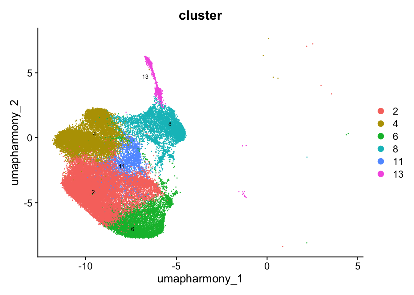
paed_sub <- paed_sub %>%
  NormalizeData() %>%
  FindVariableFeatures() %>%
  ScaleData() %>%
  RunPCA()

paed_sub <- RunUMAP(paed_sub, dims = 1:30, reduction = "pca", reduction.name = "umap.new")
meta_data_columns <- colnames(paed_sub@meta.data)
columns_to_remove <- grep("^RNA_snn_res", meta_data_columns, value = TRUE)
paed_sub@meta.data <- paed_sub@meta.data[, !(colnames(paed_sub@meta.data) %in% columns_to_remove)]resolutions <- seq(0.1, 1, by = 0.1)
paed_sub <- FindNeighbors(paed_sub, dims = 1:30, reduction = "pca")
paed_sub <- FindClusters(paed_sub, resolution = resolutions )Modularity Optimizer version 1.3.0 by Ludo Waltman and Nees Jan van Eck
Number of nodes: 42503
Number of edges: 1301848
Running Louvain algorithm...
Maximum modularity in 10 random starts: 0.9540
Number of communities: 6
Elapsed time: 6 seconds
Modularity Optimizer version 1.3.0 by Ludo Waltman and Nees Jan van Eck
Number of nodes: 42503
Number of edges: 1301848
Running Louvain algorithm...
Maximum modularity in 10 random starts: 0.9338
Number of communities: 11
Elapsed time: 6 seconds
Modularity Optimizer version 1.3.0 by Ludo Waltman and Nees Jan van Eck
Number of nodes: 42503
Number of edges: 1301848
Running Louvain algorithm...
Maximum modularity in 10 random starts: 0.9218
Number of communities: 14
Elapsed time: 6 seconds
Modularity Optimizer version 1.3.0 by Ludo Waltman and Nees Jan van Eck
Number of nodes: 42503
Number of edges: 1301848
Running Louvain algorithm...
Maximum modularity in 10 random starts: 0.9108
Number of communities: 16
Elapsed time: 6 seconds
Modularity Optimizer version 1.3.0 by Ludo Waltman and Nees Jan van Eck
Number of nodes: 42503
Number of edges: 1301848
Running Louvain algorithm...
Maximum modularity in 10 random starts: 0.9010
Number of communities: 16
Elapsed time: 6 seconds
Modularity Optimizer version 1.3.0 by Ludo Waltman and Nees Jan van Eck
Number of nodes: 42503
Number of edges: 1301848
Running Louvain algorithm...
Maximum modularity in 10 random starts: 0.8913
Number of communities: 18
Elapsed time: 5 seconds
Modularity Optimizer version 1.3.0 by Ludo Waltman and Nees Jan van Eck
Number of nodes: 42503
Number of edges: 1301848
Running Louvain algorithm...
Maximum modularity in 10 random starts: 0.8824
Number of communities: 20
Elapsed time: 7 seconds
Modularity Optimizer version 1.3.0 by Ludo Waltman and Nees Jan van Eck
Number of nodes: 42503
Number of edges: 1301848
Running Louvain algorithm...
Maximum modularity in 10 random starts: 0.8752
Number of communities: 22
Elapsed time: 6 seconds
Modularity Optimizer version 1.3.0 by Ludo Waltman and Nees Jan van Eck
Number of nodes: 42503
Number of edges: 1301848
Running Louvain algorithm...
Maximum modularity in 10 random starts: 0.8673
Number of communities: 21
Elapsed time: 6 seconds
Modularity Optimizer version 1.3.0 by Ludo Waltman and Nees Jan van Eck
Number of nodes: 42503
Number of edges: 1301848
Running Louvain algorithm...
Maximum modularity in 10 random starts: 0.8596
Number of communities: 22
Elapsed time: 6 secondsclustree(paed_sub, prefix = "RNA_snn_res.")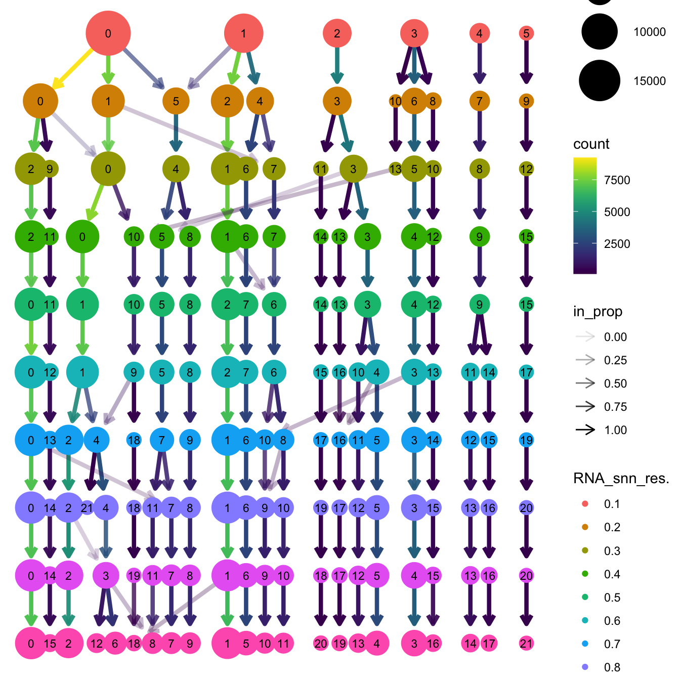
# Visualize the clustering results
DimPlot(paed_sub, group.by = "RNA_snn_res.0.4", reduction = "umap.new", label = TRUE, label.size = 2.5, repel = TRUE, raster = FALSE )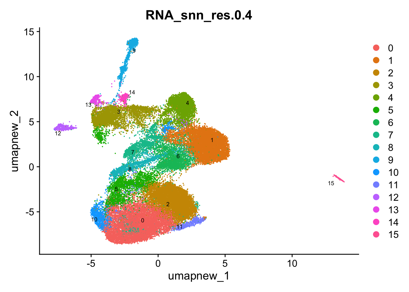
opt_res <- "RNA_snn_res.0.4"
n <- nlevels(paed_sub$RNA_snn_res.0.4)
paed_sub$RNA_snn_res.0.4 <- factor(paed_sub$RNA_snn_res.0.4, levels = seq(0,n-1))
paed_sub$seurat_clusters <- NULL
paed_sub$cluster <- paed_sub$RNA_snn_res.0.4
Idents(paed_sub) <- paed_sub$cluster
paed_sub.markers <- FindAllMarkers(paed_sub, only.pos = TRUE, min.pct = 0.25, logfc.threshold = 0.25)Calculating cluster 0Calculating cluster 1Calculating cluster 2Calculating cluster 3Calculating cluster 4Calculating cluster 5Calculating cluster 6Calculating cluster 7Calculating cluster 8Calculating cluster 9Calculating cluster 10Calculating cluster 11Calculating cluster 12Calculating cluster 13Calculating cluster 14Calculating cluster 15paed_sub.markers %>%
group_by(cluster) %>% unique() %>%
top_n(n = 5, wt = avg_log2FC) -> top5
paed_sub.markers %>%
group_by(cluster) %>%
slice_head(n=1) %>%
pull(gene) -> best.wilcox.gene.per.cluster
best.wilcox.gene.per.cluster [1] "TOX2" "KLF2" "GPR183" "CCL5" "CD8A" "MAF" "KLF2" "IFI44L"
[9] "FOXP3" "TRDC" "EGR2" "ACTB" "GZMK" "CCL5" "NKG7" "MS4A1" Violin plot shows the expression of top marker gene per cluster.
VlnPlot(paed_sub, features=best.wilcox.gene.per.cluster, ncol = 2, raster = FALSE, pt.size = FALSE)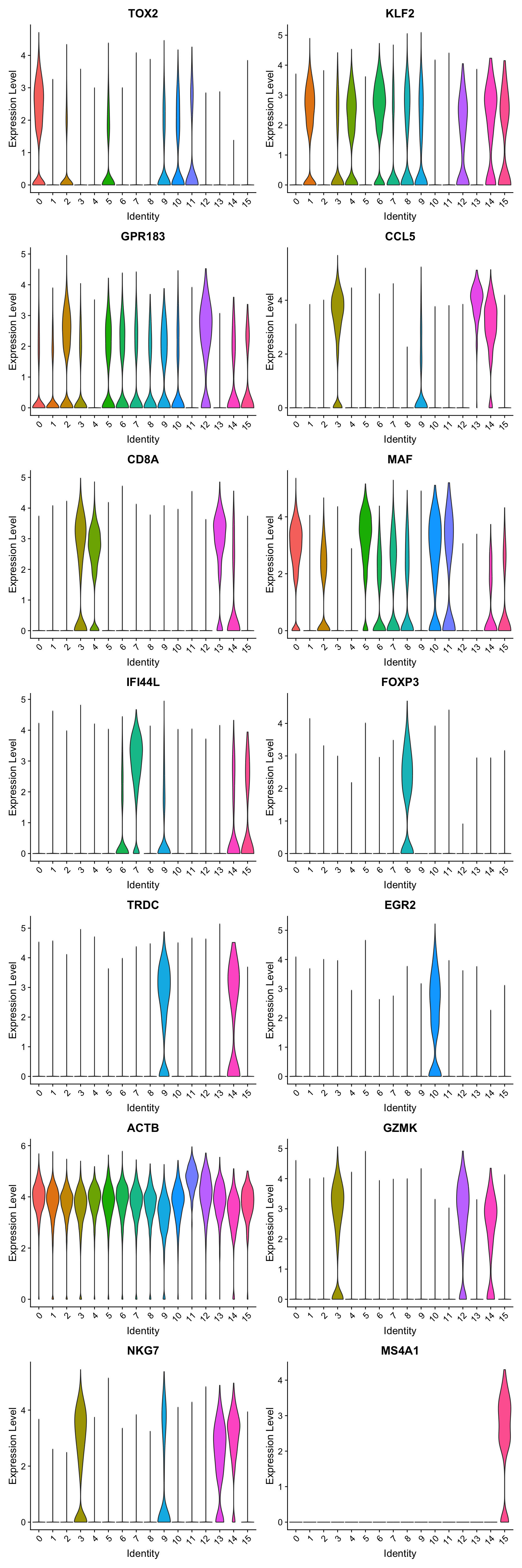
Feature plot shows the expression of top marker genes per cluster.
FeaturePlot(paed_sub,features=best.wilcox.gene.per.cluster, reduction = 'umap.new', raster = FALSE, ncol = 3, label = TRUE)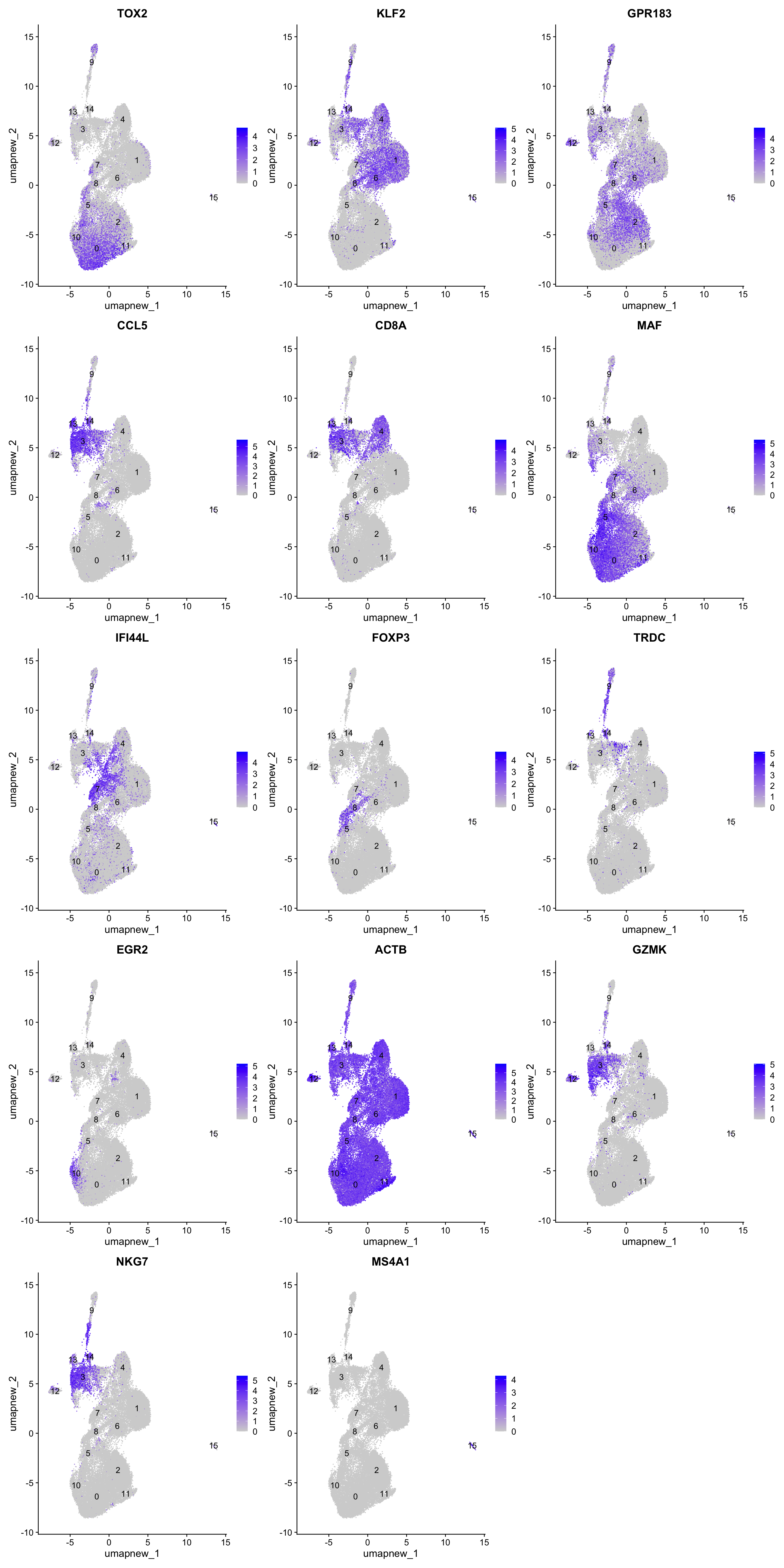
Top 10 marker genes from Seurat
## Seurat top markers
top10 <- paed_sub.markers %>%
    group_by(cluster) %>%
    top_n(n = 10, wt = avg_log2FC) %>%
    ungroup() %>%
    distinct(gene, .keep_all = TRUE) %>%
    arrange(cluster, desc(avg_log2FC))

cluster_colors <- paletteer::paletteer_d("pals::glasbey")[factor(top10$cluster)]

DotPlot(paed_sub,
        features = unique(top10$gene),
        group.by = opt_res,
        cols = c("azure1", "blueviolet"),
        dot.scale = 3, assay = "RNA") +
    RotatedAxis() +
    FontSize(y.text = 8, x.text = 12) +
    labs(y = element_blank(), x = element_blank()) +
    coord_flip() +
    theme(axis.text.y = element_text(color = cluster_colors)) +
    ggtitle("Top 10 marker genes per cluster (Seurat)")
Warning: Vectorized input to `element_text()` is not officially supported.
ℹ Results may be unexpected or may change in future versions of ggplot2.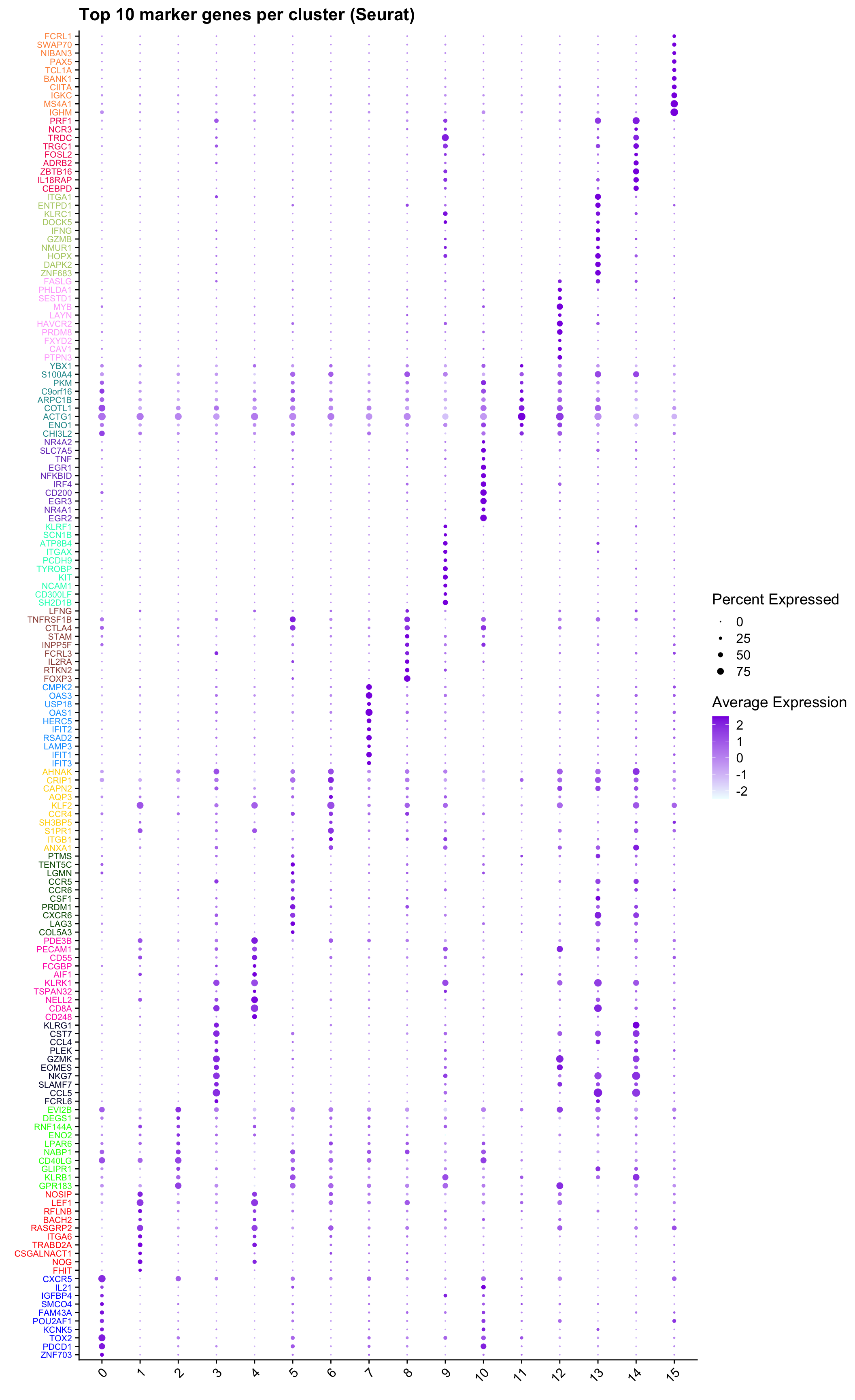
out_markers <- here("output",
            "CSV",
            paste(tissue,"_Marker_genes_Reclustered_Tcell_population.",opt_res, sep = ""))

dir.create(out_markers, recursive = TRUE, showWarnings = FALSE)

for (cl in unique(paed_sub.markers$cluster)) {
  cluster_data <- paed_sub.markers %>% dplyr::filter(cluster == cl)
  file_name <- here(out_markers, paste0("G000231_Neeland_",tissue, "_cluster_", cl, ".csv"))
  if (!file.exists(file_name)) {
  write.csv(cluster_data, file = file_name)
  }
}
Corresponding Azimuth labels (T cell subsets)
## Level 1
DimPlot(paed_sub, reduction = "umap.new", group.by = "predicted.celltype.l1", raster = FALSE, repel = TRUE, label = TRUE, label.size = 4.5) 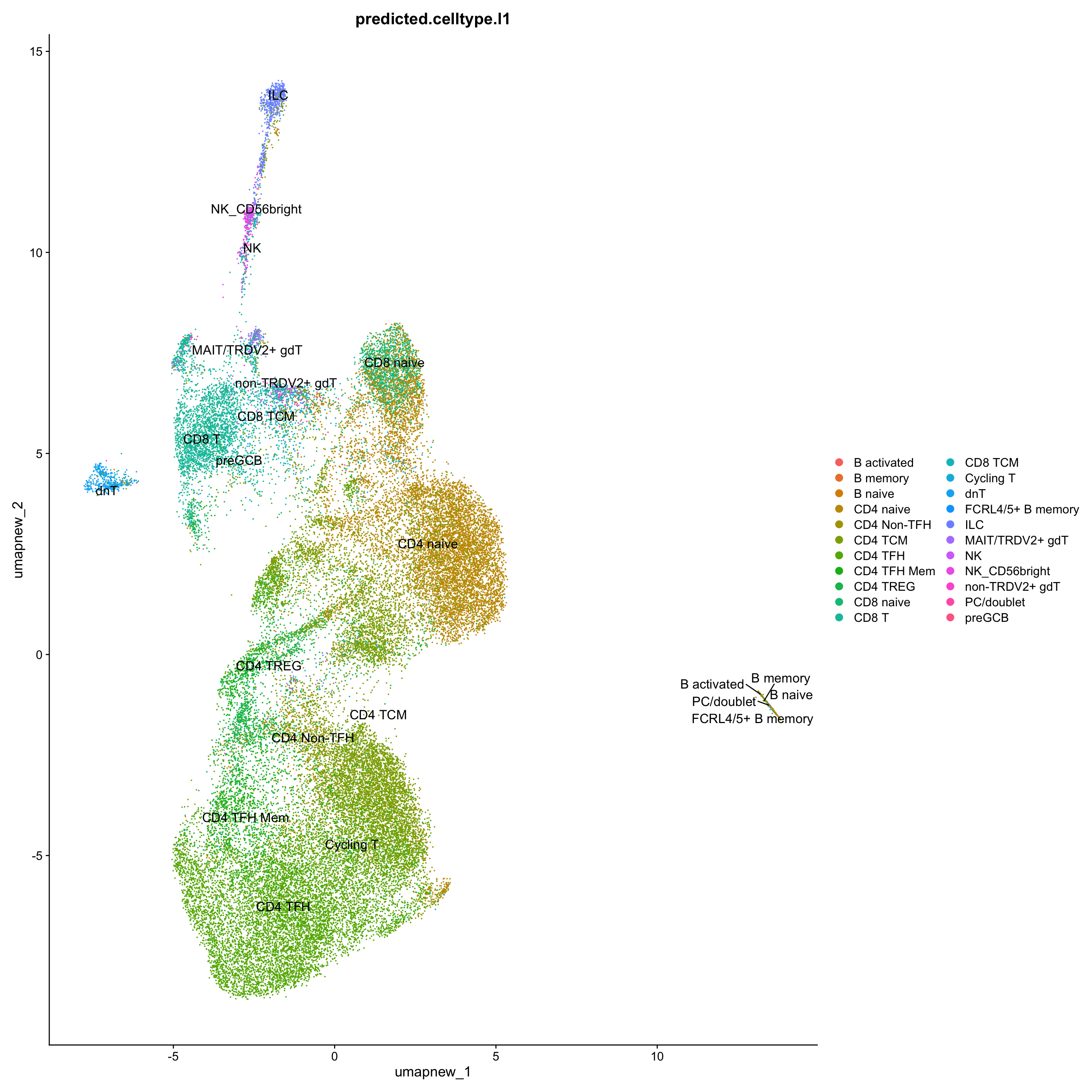
Excluding contaminating cells (B cell subtypes) for further clarity
sort(table(paed_sub$predicted.celltype.l1), decreasing = T)
          CD4 TFH           CD4 TCM         CD4 naive             CD8 T
            10935              9419              9316              2934
         CD4 TREG       CD4 TFH Mem       CD4 Non-TFH         CD8 naive
             2165              1878              1510              1408
          CD8 TCM               ILC               dnT     NK_CD56bright
              977               626               569               233
   non-TRDV2+ gdT   MAIT/TRDV2+ gdT           B naive                NK
              175               152               103                65
      B activated          B memory         Cycling T FCRL4/5+ B memory
               14                10                10                 2
       PC/doublet            preGCB
                1                 1
exclude <- c("B activated", "B memory", "B naive", "FCRL4/5+ B memory", "PC/doublet", "preGCB")
paed_sub_filtered <- paed_sub[, !paed_sub$predicted.celltype.l1 %in% exclude]
# Plots for Level 1
DimPlot(paed_sub_filtered, reduction = "umap.new", group.by = "predicted.celltype.l1", raster = FALSE, repel = TRUE, label = TRUE, label.size = 5) +
paletteer::scale_colour_paletteer_d("Polychrome::palette36")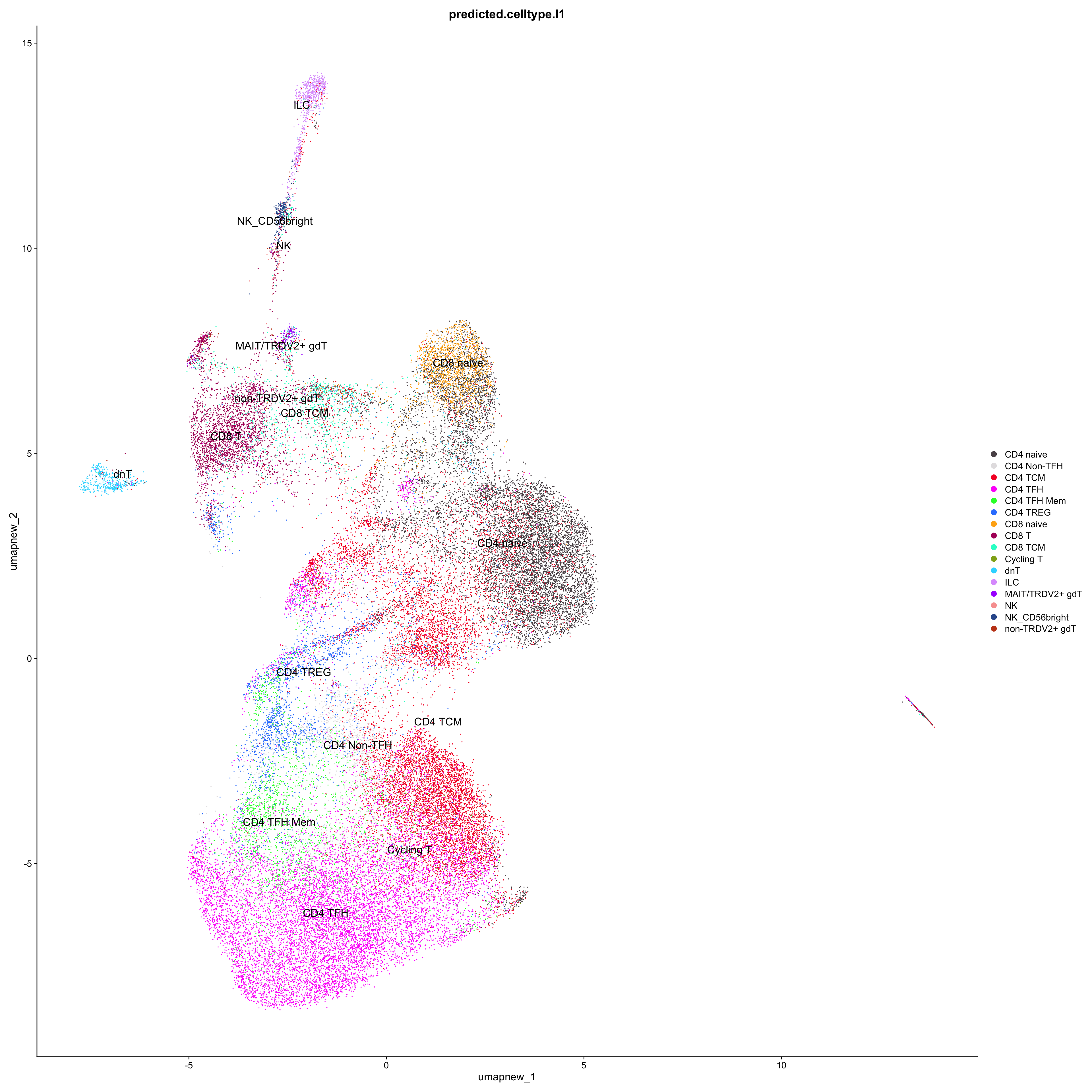
df_table_l1 <- as.data.frame(table(paed_sub_filtered$RNA_snn_res.0.4, paed_sub_filtered$predicted.celltype.l1))

ggplot(df_table_l1, aes(Var1, Freq, fill = Var2)) +
  geom_bar(stat = "identity") +
  labs(x = "RNA_snn_res.0.4", y = "Count", fill = "predicted.celltype.l1") +
  theme_minimal() +
  paletteer::scale_fill_paletteer_d("Polychrome::palette36") +
  ggtitle("Stacked Bar Plot of Tcell subsets (res=0.4) and predicted.celltype.l1")
# Plots for Level 2
DimPlot(paed_sub_filtered, reduction = "umap.new", group.by = "predicted.celltype.l2", raster = FALSE, repel = TRUE, label = TRUE, label.size = 5)  +
    paletteer::scale_colour_paletteer_d("Polychrome::palette36")
df_table_l2 <- as.data.frame(table(paed_sub_filtered$RNA_snn_res.0.4, paed_sub_filtered$predicted.celltype.l2))

ggplot(df_table_l2, aes(Var1, Freq, fill = Var2)) +
  geom_bar(stat = "identity") +
  labs(x = "RNA_snn_res.0.4", y = "Count", fill = "predicted.celltype.l2") +
  theme_minimal() +
  paletteer::scale_fill_paletteer_d("Polychrome::palette36") +
  ggtitle("Stacked Bar Plot of Tcell subsets (res=0.4) and predicted.celltype.l2")
Update T subclustering labels
cell_labels <- readxl::read_excel(here("data/Cell_labels_Mel_v2/earlyAIR_Tonsil_and_Adenoid_T-NK_annotations_17.07.24.xlsx"), sheet = "Adenoid")
new_cluster_names <- cell_labels %>%
  dplyr::select(cluster, annotation) %>%
  deframe()

paed_sub <- RenameIdents(paed_sub, new_cluster_names)
paed_sub@meta.data$cell_labels_v2 <- Idents(paed_sub)

DimPlot(paed_sub, reduction = "umap.new", raster = FALSE, repel = TRUE, label = TRUE, label.size = 3.5) + ggtitle(paste0(tissue, ": UMAP with Updated subclustering"))
palette1 <- paletteer::paletteer_d("ggthemes::Classic_20")
palette2 <- paletteer::paletteer_d("Polychrome::light")
combined_palette <- unique(c(palette1, palette2))

labels <- c("cell_labels", "cell_labels_v2", "RNA_snn_res.0.4")

p <- vector("list",length(labels))
for(label in labels){
  paed_sub@meta.data %>%
    ggplot(aes(x = !!sym(label),
               fill = !!sym(label))) +
    geom_bar() +
    geom_text(aes(label = ..count..), stat = "count",
              vjust = -0.5, colour = "black", size = 2) +
    scale_y_log10() +
    theme(axis.text.x = element_blank(),
          axis.title.x = element_blank(),
          axis.ticks.x = element_blank()) +
    NoLegend() +
    labs(y = "No. Cells (log scale)") -> p1

  paed_sub@meta.data %>%
    dplyr::select(!!sym(label), Sample) %>%
    group_by(!!sym(label), Sample) %>%
    summarise(num = n()) %>%
    mutate(prop = num / sum(num)) %>%
  ggplot(aes(x = !!sym(label), y = prop * 100,
             fill = Sample)) +
    geom_bar(stat = "identity") +
    theme(axis.text.x = element_text(angle = 90,
                                     vjust = 0.5,
                                     hjust = 1,
                                     size = 8)) +
    labs(y = "% Cells", fill = "Sample") +
  scale_fill_manual(values = combined_palette) -> p2

  (p1 / p2) & theme(legend.text = element_text(size = 8),
                  legend.key.size = unit(3, "mm")) -> p[[label]]
}
`summarise()` has grouped output by 'cell_labels'. You can override using the
`.groups` argument.
`summarise()` has grouped output by 'cell_labels_v2'. You can override using
the `.groups` argument.
`summarise()` has grouped output by 'RNA_snn_res.0.4'. You can override using
the `.groups` argument.p[[1]]
NULL
[[2]]
NULL
[[3]]
NULL
$cell_labelsWarning: The dot-dot notation (`..count..`) was deprecated in ggplot2 3.4.0.
ℹ Please use `after_stat(count)` instead.
This warning is displayed once every 8 hours.
Call `lifecycle::last_lifecycle_warnings()` to see where this warning was
generated.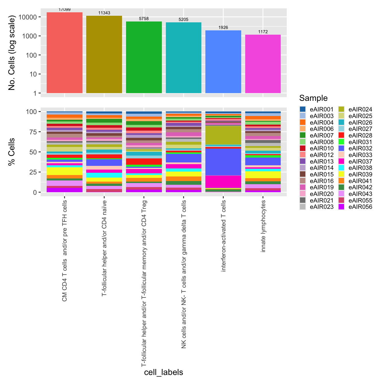
$cell_labels_v2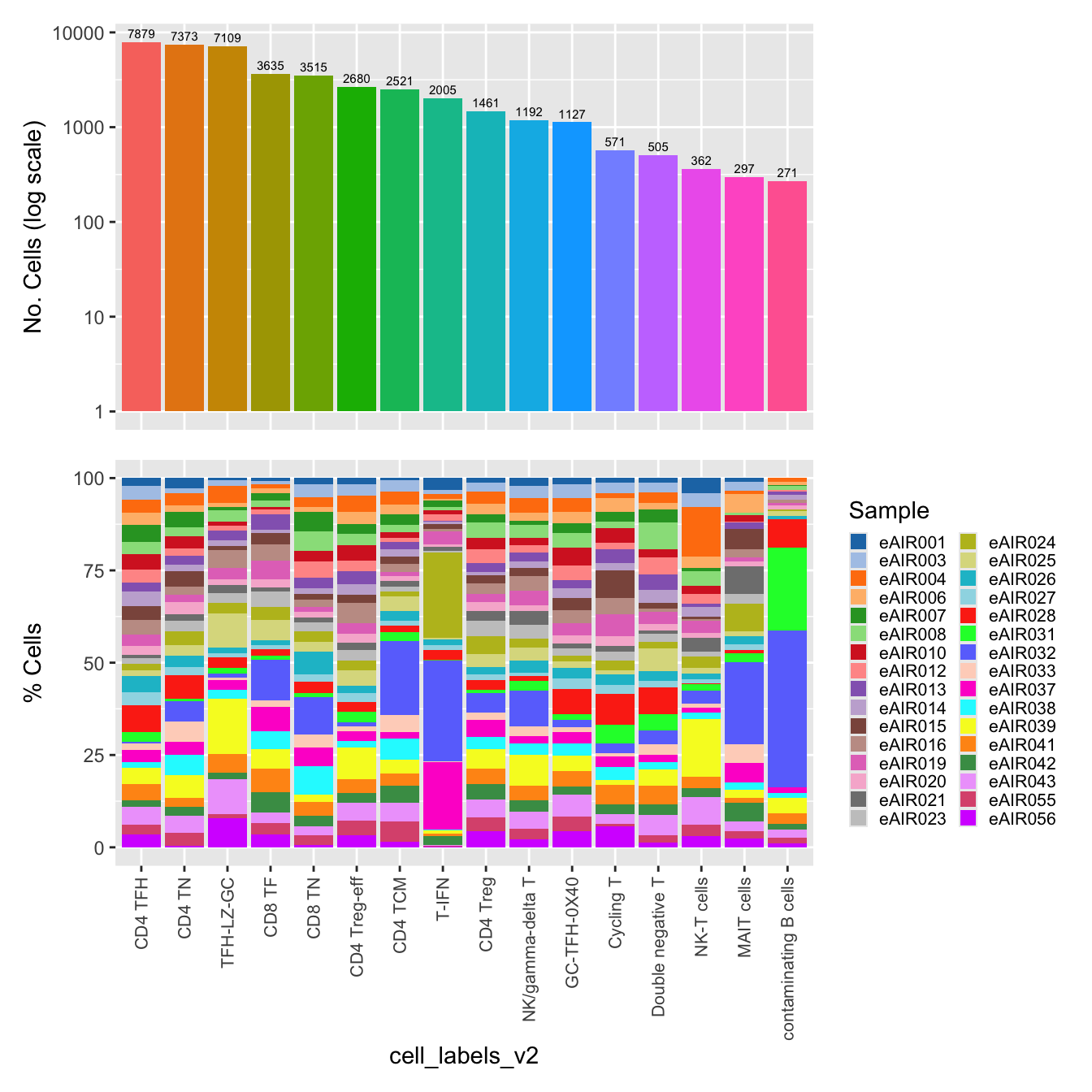
$RNA_snn_res.0.4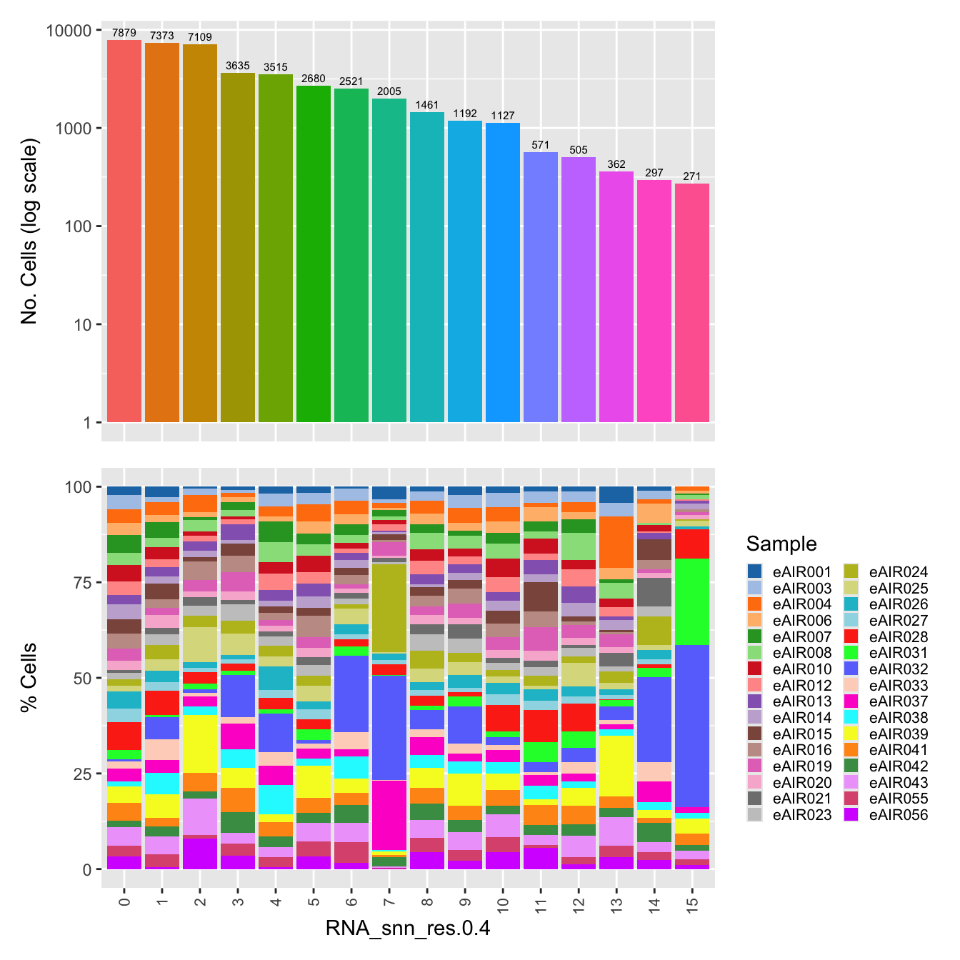
Save subclustered SEU object (Tcells)
out2 <- here("output",
            "RDS", "AllBatches_Subclustering_SEUs", tissue,
             paste0("G000231_Neeland_",tissue,".Tcell_population.subclusters.SEU.rds"))
#dir.create(out2)
if (!file.exists(out2)) {
  saveRDS(paed_sub, file = out2)
}
Reclustering Germinal Center B cells
Reclustering clusters 3,5,9
The marker genes for this reclustering can be found here-
Adenoids_GC_population_res.0.6
sub_clusters <- c(3,5,9)

idx <- which(merged_obj$cluster %in% sub_clusters)
paed_sub <- merged_obj[,idx]
paed_sub
An object of class Seurat
17456 features across 25451 samples within 1 assay
Active assay: RNA (17456 features, 2000 variable features)
3 layers present: data, counts, scale.data
4 dimensional reductions calculated: pca, umap.unintegrated, harmony, umap.harmony# Visualize the clustering results
DimPlot(paed_sub, reduction = "umap.harmony", group.by = "cluster", label = TRUE, label.size = 2.5, repel = TRUE, raster = FALSE )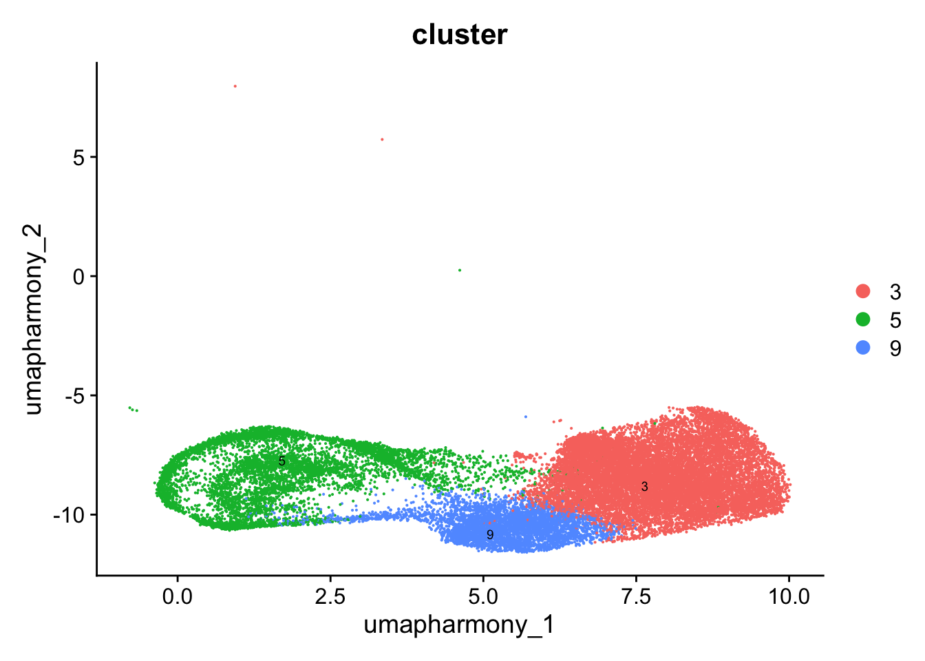
paed_sub <- paed_sub %>%
  NormalizeData() %>%
  FindVariableFeatures() %>%
  ScaleData() %>%
  RunPCA()

paed_sub <- RunUMAP(paed_sub, dims = 1:30, reduction = "pca", reduction.name = "umap.new")
meta_data_columns <- colnames(paed_sub@meta.data)
columns_to_remove <- grep("^RNA_snn_res", meta_data_columns, value = TRUE)
paed_sub@meta.data <- paed_sub@meta.data[, !(colnames(paed_sub@meta.data) %in% columns_to_remove)]resolutions <- seq(0.1, 1, by = 0.1)
paed_sub <- FindNeighbors(paed_sub, dims = 1:30, reduction = "pca")
paed_sub <- FindClusters(paed_sub, resolution = resolutions )Modularity Optimizer version 1.3.0 by Ludo Waltman and Nees Jan van Eck
Number of nodes: 25451
Number of edges: 785374
Running Louvain algorithm...
Maximum modularity in 10 random starts: 0.9400
Number of communities: 3
Elapsed time: 3 seconds
Modularity Optimizer version 1.3.0 by Ludo Waltman and Nees Jan van Eck
Number of nodes: 25451
Number of edges: 785374
Running Louvain algorithm...
Maximum modularity in 10 random starts: 0.9065
Number of communities: 5
Elapsed time: 4 seconds
Modularity Optimizer version 1.3.0 by Ludo Waltman and Nees Jan van Eck
Number of nodes: 25451
Number of edges: 785374
Running Louvain algorithm...
Maximum modularity in 10 random starts: 0.8875
Number of communities: 7
Elapsed time: 4 seconds
Modularity Optimizer version 1.3.0 by Ludo Waltman and Nees Jan van Eck
Number of nodes: 25451
Number of edges: 785374
Running Louvain algorithm...
Maximum modularity in 10 random starts: 0.8694
Number of communities: 8
Elapsed time: 3 seconds
Modularity Optimizer version 1.3.0 by Ludo Waltman and Nees Jan van Eck
Number of nodes: 25451
Number of edges: 785374
Running Louvain algorithm...
Maximum modularity in 10 random starts: 0.8567
Number of communities: 10
Elapsed time: 3 seconds
Modularity Optimizer version 1.3.0 by Ludo Waltman and Nees Jan van Eck
Number of nodes: 25451
Number of edges: 785374
Running Louvain algorithm...
Maximum modularity in 10 random starts: 0.8463
Number of communities: 13
Elapsed time: 3 seconds
Modularity Optimizer version 1.3.0 by Ludo Waltman and Nees Jan van Eck
Number of nodes: 25451
Number of edges: 785374
Running Louvain algorithm...
Maximum modularity in 10 random starts: 0.8357
Number of communities: 15
Elapsed time: 3 seconds
Modularity Optimizer version 1.3.0 by Ludo Waltman and Nees Jan van Eck
Number of nodes: 25451
Number of edges: 785374
Running Louvain algorithm...
Maximum modularity in 10 random starts: 0.8249
Number of communities: 15
Elapsed time: 3 seconds
Modularity Optimizer version 1.3.0 by Ludo Waltman and Nees Jan van Eck
Number of nodes: 25451
Number of edges: 785374
Running Louvain algorithm...
Maximum modularity in 10 random starts: 0.8173
Number of communities: 17
Elapsed time: 3 seconds
Modularity Optimizer version 1.3.0 by Ludo Waltman and Nees Jan van Eck
Number of nodes: 25451
Number of edges: 785374
Running Louvain algorithm...
Maximum modularity in 10 random starts: 0.8088
Number of communities: 16
Elapsed time: 3 secondsclustree(paed_sub, prefix = "RNA_snn_res.")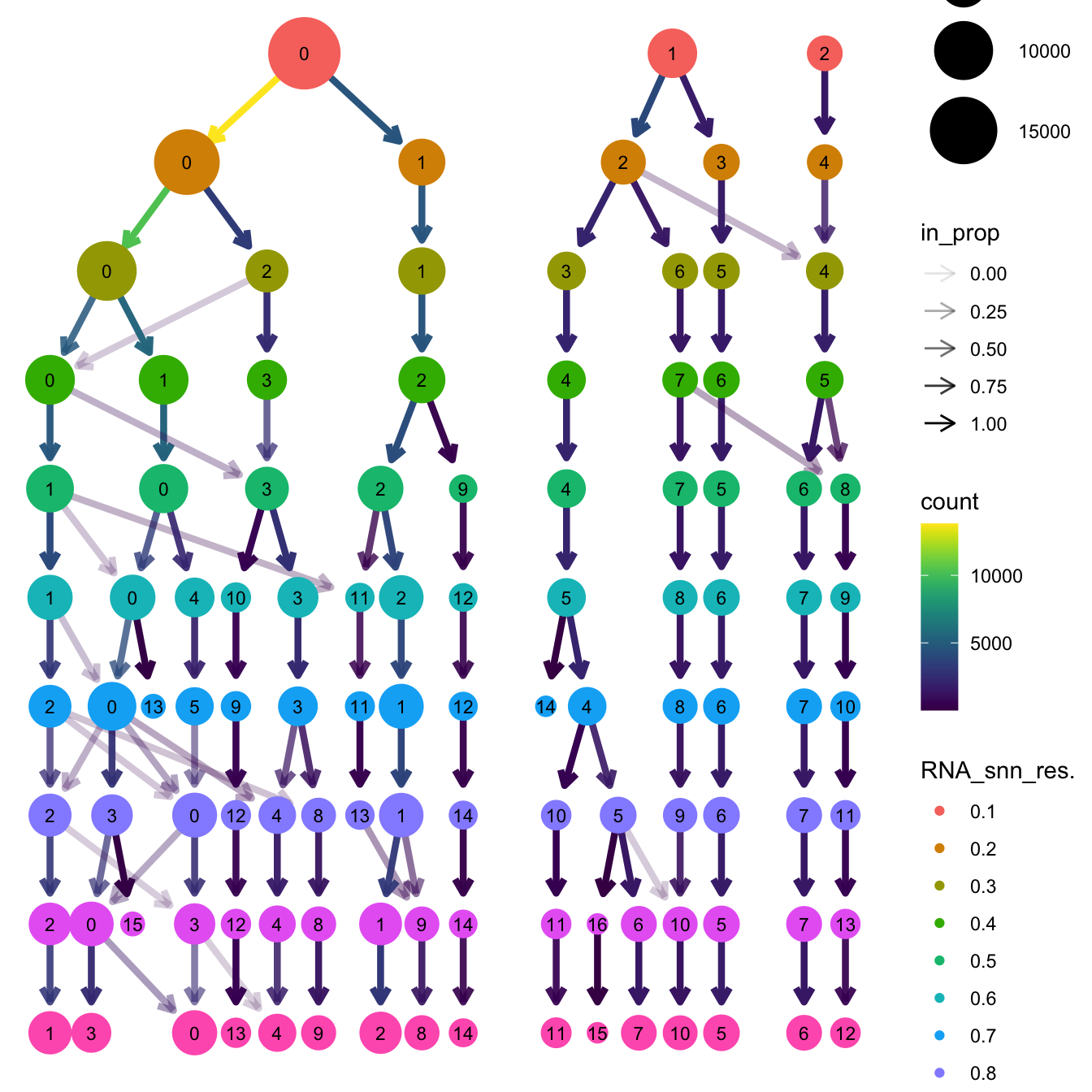
# Visualize the clustering results
DimPlot(paed_sub, group.by = "RNA_snn_res.0.6", reduction = "umap.new", label = TRUE, label.size = 2.5, repel = TRUE, raster = FALSE )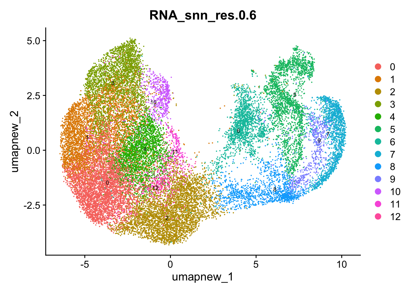
opt_res <- "RNA_snn_res.0.6"
n <- nlevels(paed_sub$RNA_snn_res.0.6)
paed_sub$RNA_snn_res.0.6 <- factor(paed_sub$RNA_snn_res.0.6, levels = seq(0,n-1))
paed_sub$seurat_clusters <- NULL
paed_sub$cluster <- paed_sub$RNA_snn_res.0.6
Idents(paed_sub) <- paed_sub$cluster
paed_sub.markers <- FindAllMarkers(paed_sub, only.pos = TRUE, min.pct = 0.25, logfc.threshold = 0.25)Calculating cluster 0Calculating cluster 1Calculating cluster 2Calculating cluster 3Calculating cluster 4Calculating cluster 5Calculating cluster 6Calculating cluster 7Calculating cluster 8Calculating cluster 9Calculating cluster 10Calculating cluster 11Calculating cluster 12paed_sub.markers %>%
group_by(cluster) %>% unique() %>%
top_n(n = 5, wt = avg_log2FC) -> top5
paed_sub.markers %>%
group_by(cluster) %>%
slice_head(n=1) %>%
pull(gene) -> best.wilcox.gene.per.cluster
best.wilcox.gene.per.cluster [1] "LMO2" "DDIT4" "AICDA" "BCL2A1" "CAMK1" "TYMS"
[7] "MCM4" "HIST1H2BB" "CDC20" "MKI67" "PRDM1" "RAB15"
[13] "PSAT1" Feature plot shows the expression of top marker genes per cluster.
FeaturePlot(paed_sub,features=best.wilcox.gene.per.cluster, reduction = 'umap.new', raster = FALSE, ncol = 2, label = TRUE)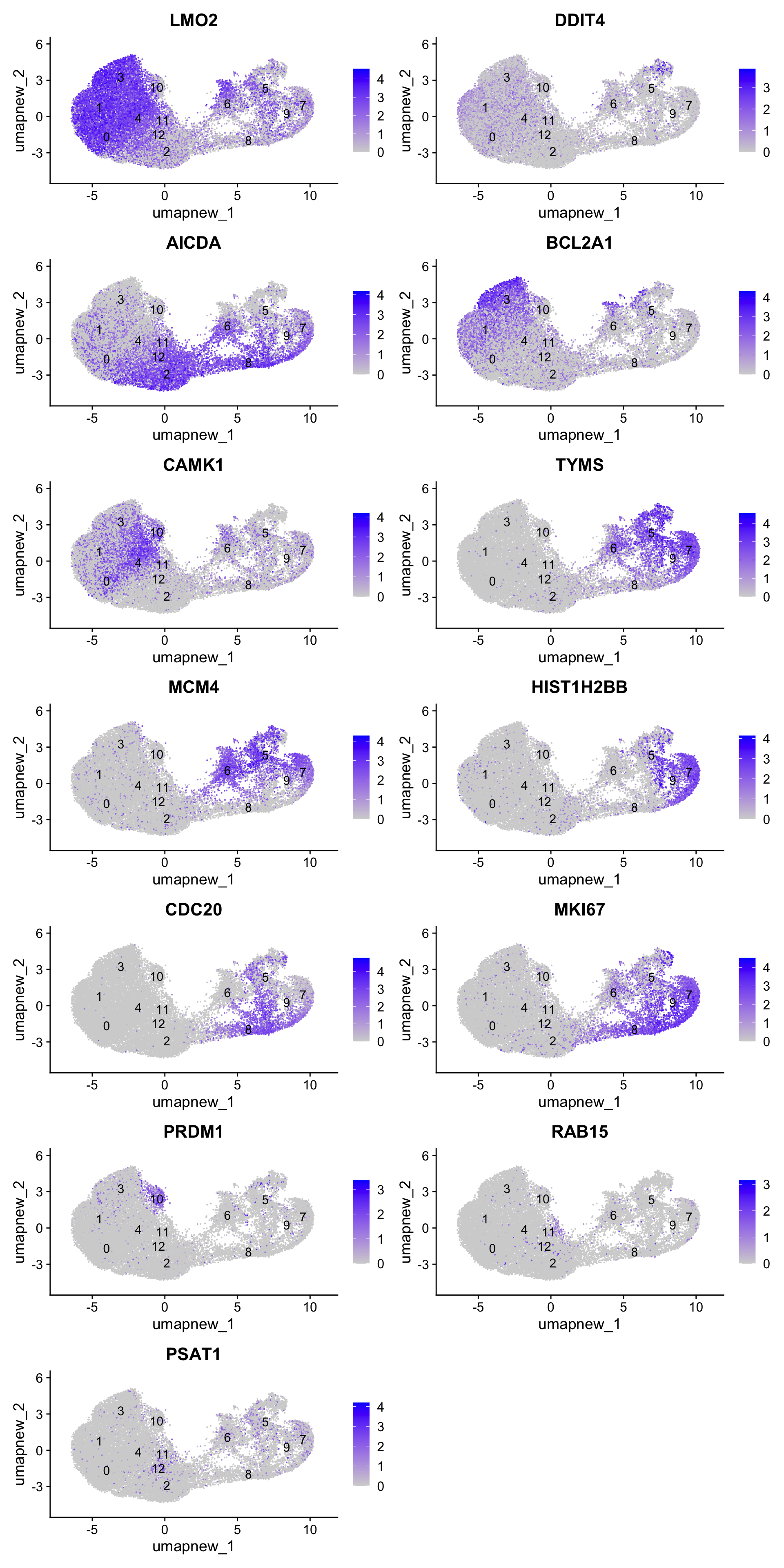
Top 10 marker genes from Seurat
## Seurat top markers
top10 <- paed_sub.markers %>%
    group_by(cluster) %>%
    top_n(n = 10, wt = avg_log2FC) %>%
    ungroup() %>%
    distinct(gene, .keep_all = TRUE) %>%
    arrange(cluster, desc(avg_log2FC))

cluster_colors <- paletteer::paletteer_d("pals::glasbey")[factor(top10$cluster)]

DotPlot(paed_sub,
        features = unique(top10$gene),
        group.by = opt_res,
        cols = c("azure1", "blueviolet"),
        dot.scale = 3, assay = "RNA") +
    RotatedAxis() +
    FontSize(y.text = 8, x.text = 12) +
    labs(y = element_blank(), x = element_blank()) +
    coord_flip() +
    theme(axis.text.y = element_text(color = cluster_colors)) +
    ggtitle("Top 10 marker genes per cluster (Seurat)")
Warning: Vectorized input to `element_text()` is not officially supported.
ℹ Results may be unexpected or may change in future versions of ggplot2.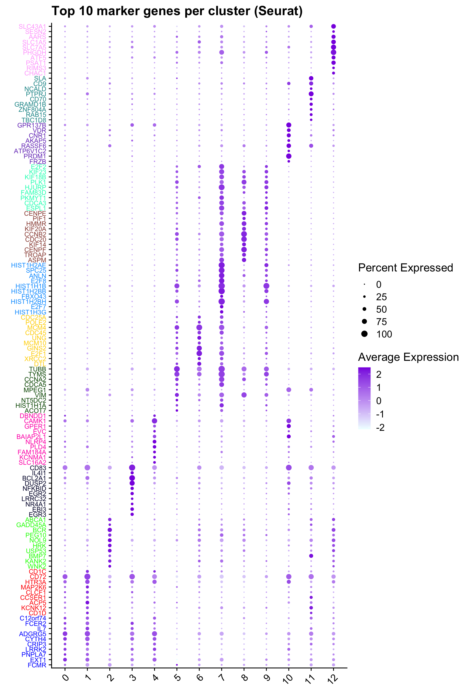
out_markers <- here("output",
            "CSV",
            paste(tissue,"_Marker_genes_Reclustered_GC_population.",opt_res, sep = ""))

dir.create(out_markers, recursive = TRUE, showWarnings = FALSE)

for (cl in unique(paed_sub.markers$cluster)) {
  cluster_data <- paed_sub.markers %>% dplyr::filter(cluster == cl)
  file_name <- here(out_markers, paste0("G000231_Neeland_",tissue, "_cluster_", cl, ".csv"))
  write.csv(cluster_data, file = file_name)
}
Corresponding Azimuth labels (GC cell subsets)
## Level 1
DimPlot(paed_sub, reduction = "umap.new", group.by = "predicted.celltype.l1", raster = FALSE, repel = TRUE, label = TRUE, label.size = 4.5) 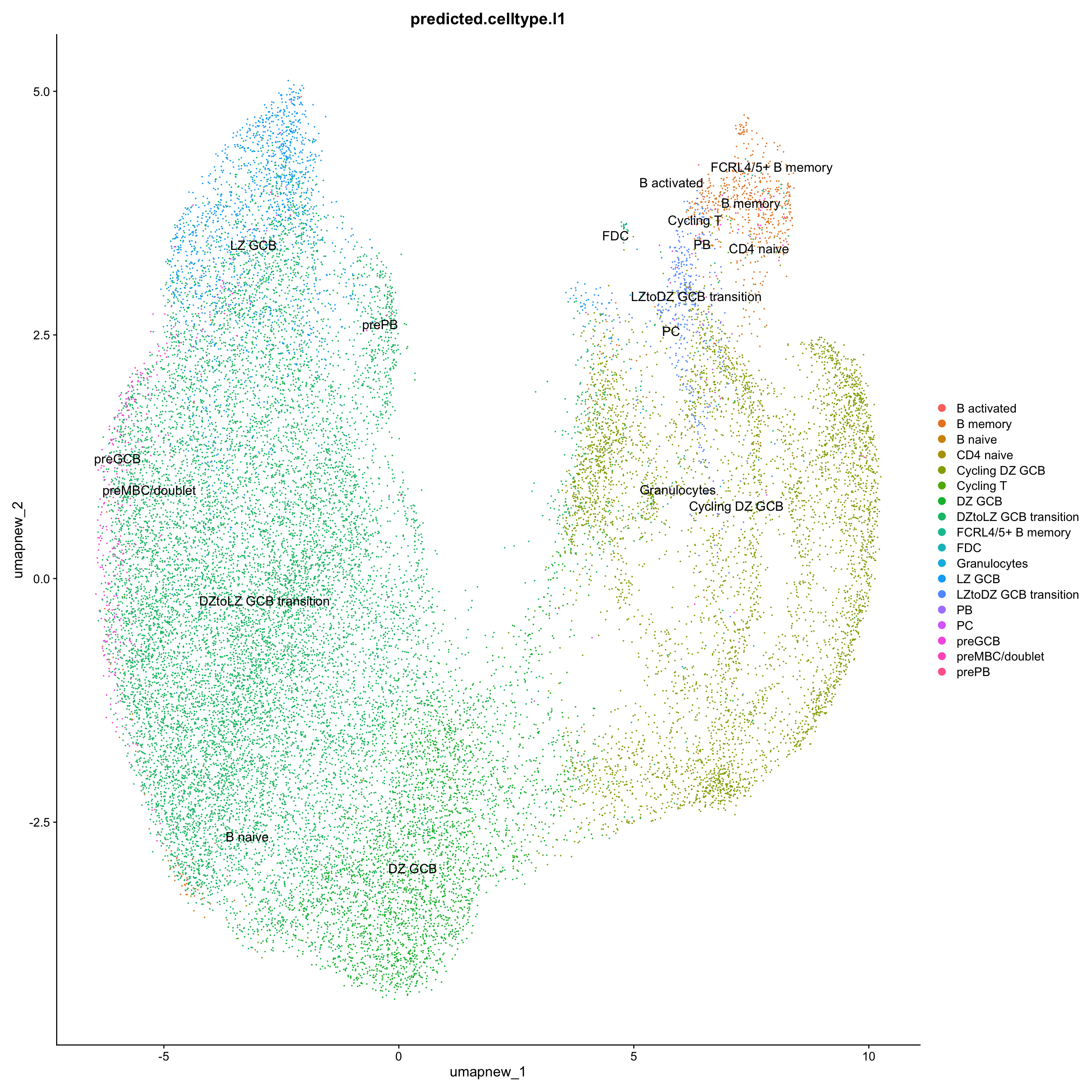
df_table <- as.data.frame(table(paed_sub$RNA_snn_res.0.6, paed_sub$predicted.celltype.l1))
ggplot(df_table, aes(Var1, Freq, fill = Var2)) +
  geom_bar(stat = "identity") +
  labs(x = "RNA_snn_res.0.6", y = "Count", fill = "predicted.celltype.l1") +
  theme_minimal() +
  ggtitle("Stacked Bar Plot of Tcell subsets (res=0.6) and predicted.celltype.l1")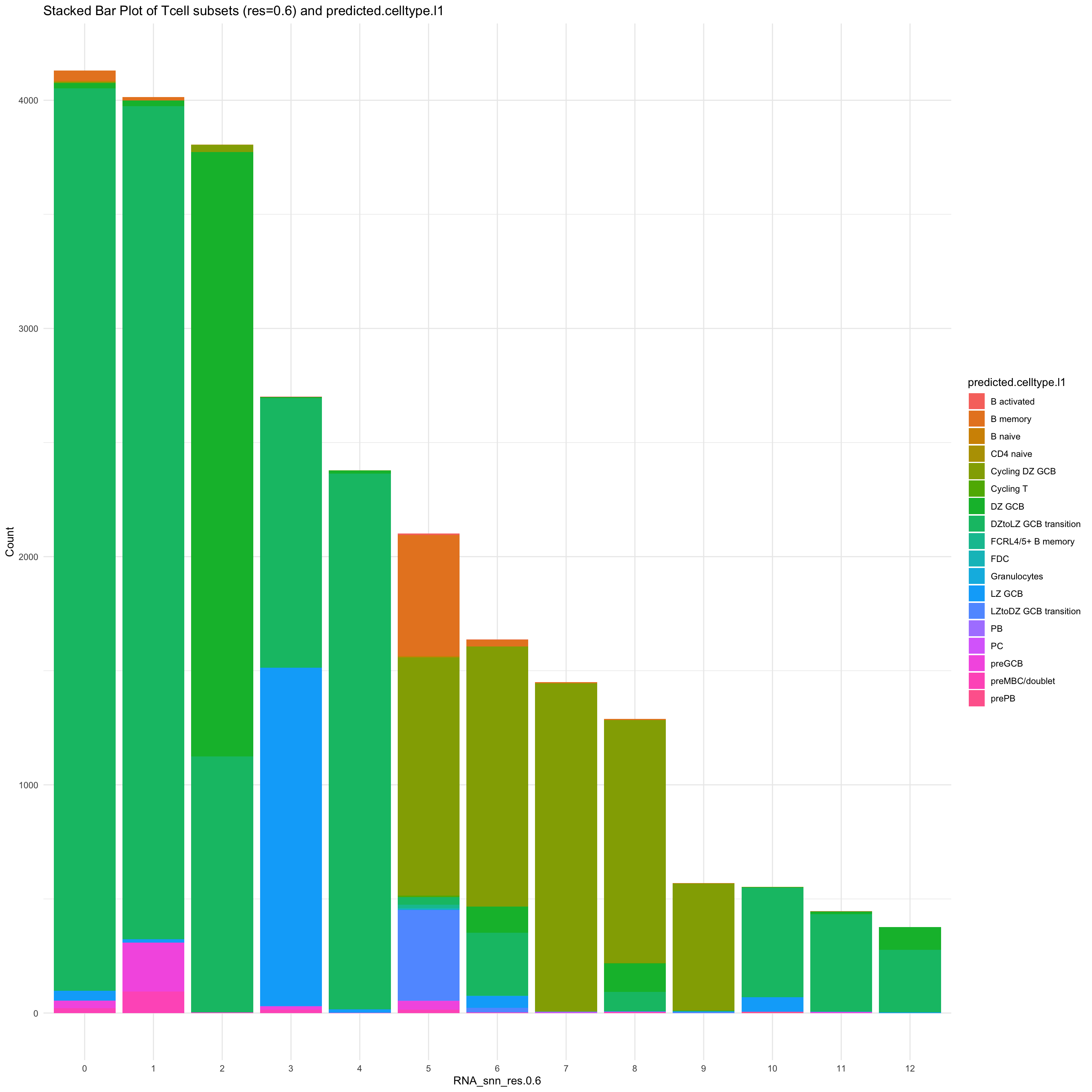
Update GC subclustering labels
cell_labels <- readxl::read_excel(here("data/Cell_labels_Mel_v2/earlyAIR_Tonsil_and_Adenoid_GC-B cell annotations_09.08.24.xlsx"), sheet = "Adenoid")
new_cluster_names <- cell_labels %>%
  dplyr::select(cluster, annotation) %>%
  deframe()

paed_sub <- RenameIdents(paed_sub, new_cluster_names)
paed_sub@meta.data$cell_labels_v2 <- Idents(paed_sub)

DimPlot(paed_sub, reduction = "umap.new", raster = FALSE, repel = TRUE, label = TRUE, label.size = 3.5) + ggtitle(paste0(tissue, ": UMAP with Updated subclustering"))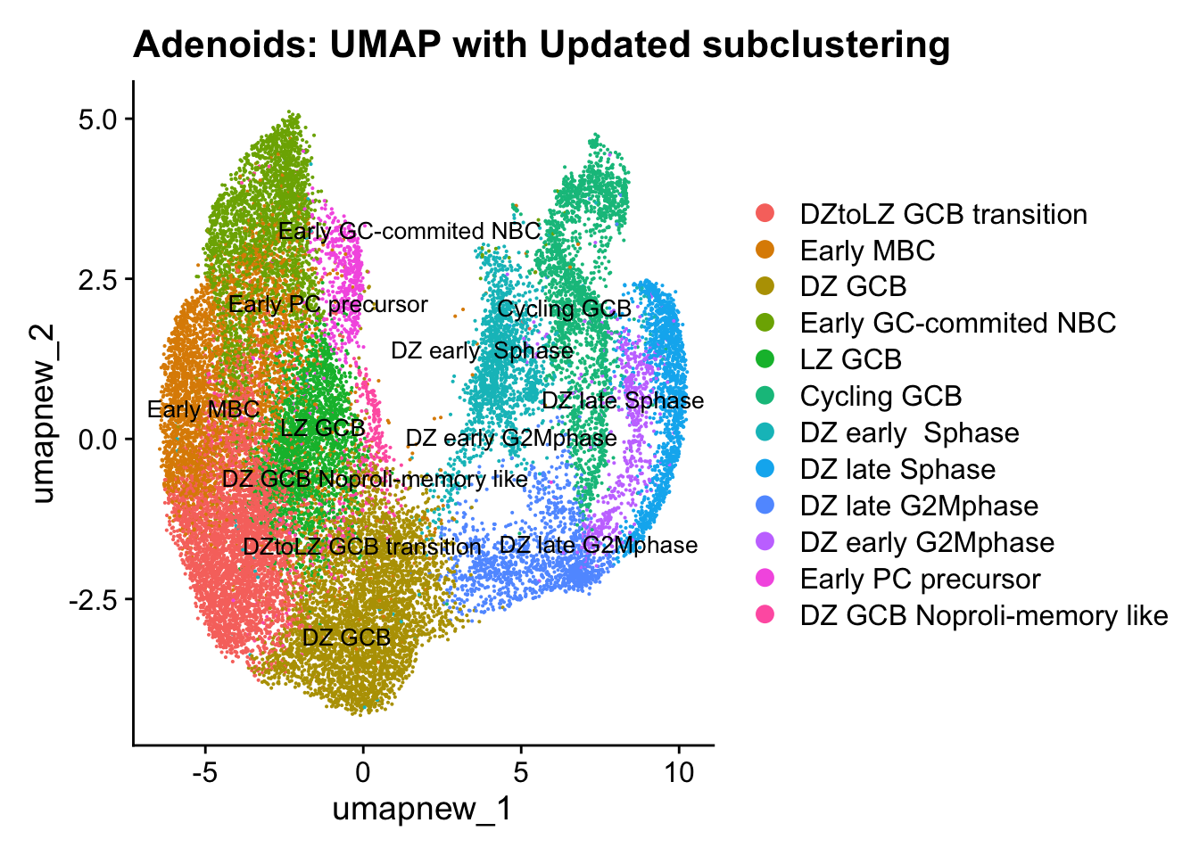
palette1 <- paletteer::paletteer_d("ggthemes::Classic_20")
palette2 <- paletteer::paletteer_d("Polychrome::light")
combined_palette <- unique(c(palette1, palette2))

labels <- c( "cell_labels", "cell_labels_v2", "RNA_snn_res.0.6")

p <- vector("list",length(labels))
for(label in labels){
  paed_sub@meta.data %>%
    ggplot(aes(x = !!sym(label),
               fill = !!sym(label))) +
    geom_bar() +
    geom_text(aes(label = ..count..), stat = "count",
              vjust = -0.5, colour = "black", size = 2) +
    scale_y_log10() +
    theme(axis.text.x = element_blank(),
          axis.title.x = element_blank(),
          axis.ticks.x = element_blank()) +
    NoLegend() +
    labs(y = "No. Cells (log scale)") -> p1

  paed_sub@meta.data %>%
    dplyr::select(!!sym(label), Sample) %>%
    group_by(!!sym(label), Sample) %>%
    summarise(num = n()) %>%
    mutate(prop = num / sum(num)) %>%
  ggplot(aes(x = !!sym(label), y = prop * 100,
             fill = Sample)) +
    geom_bar(stat = "identity") +
    theme(axis.text.x = element_text(angle = 90,
                                     vjust = 0.5,
                                     hjust = 1,
                                     size = 8)) +
    labs(y = "% Cells", fill = "Sample") +
  scale_fill_manual(values = combined_palette) -> p2

  (p1 / p2) & theme(legend.text = element_text(size = 8),
                  legend.key.size = unit(3, "mm")) -> p[[label]]
}
`summarise()` has grouped output by 'cell_labels'. You can override using the
`.groups` argument.
`summarise()` has grouped output by 'cell_labels_v2'. You can override using
the `.groups` argument.
`summarise()` has grouped output by 'RNA_snn_res.0.6'. You can override using
the `.groups` argument.p[[1]]
NULL
[[2]]
NULL
[[3]]
NULL
$cell_labels
$cell_labels_v2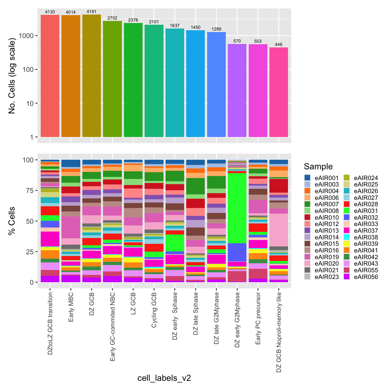
$RNA_snn_res.0.6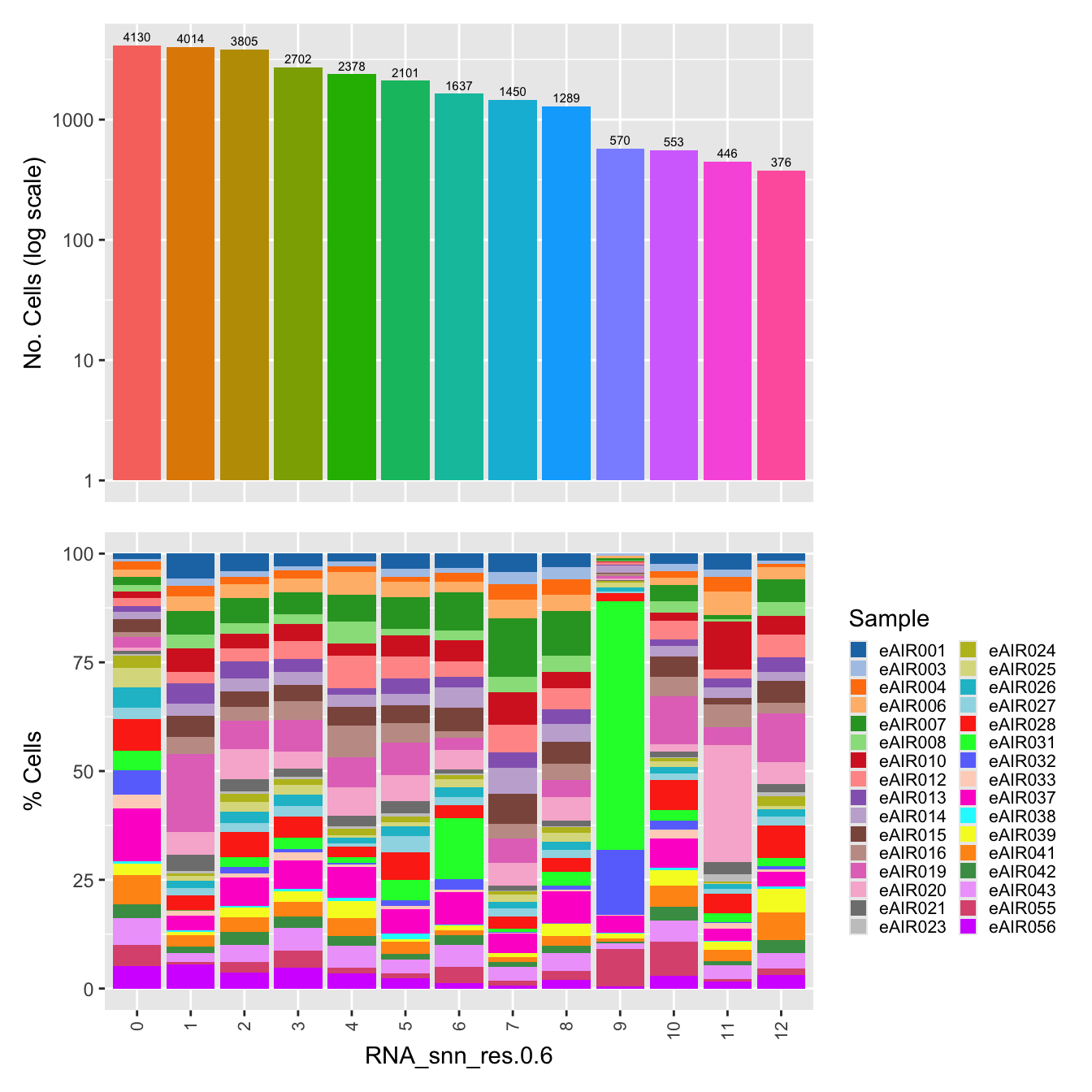
Save subclustered SEU object
out2 <- here("output",
            "RDS", "AllBatches_Subclustering_SEUs", tissue,
             paste0("G000231_Neeland_",tissue,".GC_population.subclusters.SEU.rds"))
#dir.create(out2)
if (!file.exists(out2)) {
  saveRDS(paed_sub, file = out2)
}
Confirm cluster 14 (activated DC3)
From Mel’s notes: Confirming CCR7 and LAMP3 expression in cluster 14 currently labelled as “activated DC3 (aDC3)?”
idx <- which(merged_obj$cluster %in% 14)
paed_sub <- merged_obj[,idx]
paed_sub
An object of class Seurat
17456 features across 859 samples within 1 assay
Active assay: RNA (17456 features, 2000 variable features)
3 layers present: data, counts, scale.data
4 dimensional reductions calculated: pca, umap.unintegrated, harmony, umap.harmonyFeaturePlot(paed_sub,features=c("CCR7","LAMP3"), reduction = 'umap.harmony', ncol = 1, label = FALSE)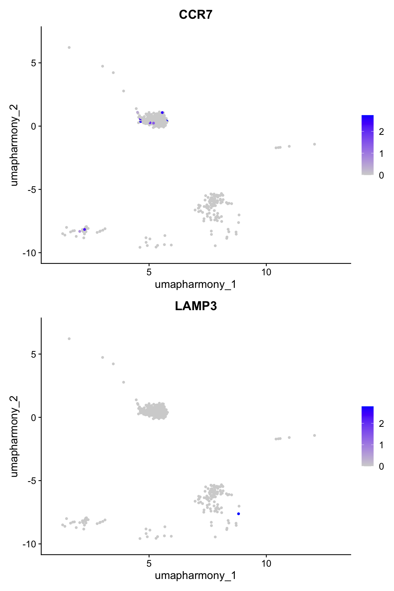
Other Clusters (excluding subclusters)
sub_clusters <- c(2,4,6,8,11,13, 3,5,9)

idx <- which(merged_obj$cluster %in% sub_clusters)
paed_other <- merged_obj[,-idx]
paed_other
An object of class Seurat
17456 features across 57002 samples within 1 assay
Active assay: RNA (17456 features, 2000 variable features)
3 layers present: data, counts, scale.data
4 dimensional reductions calculated: pca, umap.unintegrated, harmony, umap.harmonylevels(paed_other$cell_labels)[levels(paed_other$cell_labels) == "activated DC3 (aDC3)?"] <- "activated DC3 (aDC3)"
levels(Idents(paed_other))[levels(Idents(paed_other)) == "activated DC3 (aDC3)?"] <- "activated DC3 (aDC3)"
paed_other$cell_labels_v2 <- Idents(paed_other)# Visualize the clustering results
DimPlot(paed_other, reduction = "umap.harmony", group.by = "cluster", label = TRUE, label.size = 2.5, repel = TRUE, raster = FALSE )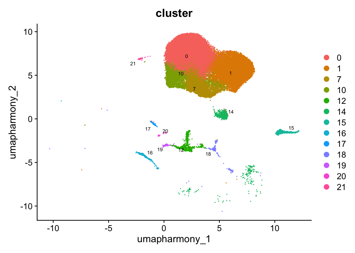
DimPlot(paed_other, reduction = "umap.harmony", label = TRUE, label.size = 2.5, repel = TRUE, raster = FALSE )
Save subclustered SEU object ( All other cells)
out2 <- here("output",
            "RDS", "AllBatches_Subclustering_SEUs", tissue,
             paste0("G000231_Neeland_",tissue,".all_other.subclusters.SEU.rds"))
#dir.create(out2)
if (!file.exists(out2)) {
  saveRDS(paed_other, file = out2)
}
Merge seurat objects of subclusters
files <- list.files(here("output",
            "RDS", "AllBatches_Subclustering_SEUs", tissue),
                    full.names = TRUE)

seuLst <- lapply(files, function(f) readRDS(f))

seu <- merge(seuLst[[1]],
             y = c(seuLst[[2]],
                   seuLst[[3]]))
seu
An object of class Seurat
17456 features across 124685 samples within 1 assay
Active assay: RNA (17456 features, 2000 variable features)
9 layers present: data.1, data.2, data.3, counts.1, scale.data.1, counts.2, scale.data.2, counts.3, scale.data.3merged <- seu %>%
NormalizeData() %>%
FindVariableFeatures() %>%
ScaleData() %>%
RunPCA()Normalizing layer: counts.1Normalizing layer: counts.2Normalizing layer: counts.3Finding variable features for layer counts.1Finding variable features for layer counts.2Finding variable features for layer counts.3Centering and scaling data matrixPC_ 1
Positive: MKI67, KIFC1, TYMS, AURKB, NUSAP1, CDK1, TOP2A, TK1, NCAPG, RRM2
HIST1H1B, TPX2, STMN1, BIRC5, HJURP, FOXM1, CCNB2, ZWINT, MYBL2, KIF11
HMGB2, KIF2C, ASF1B, CCNA2, CDCA8, UHRF1, SPC25, KIF23, CDC20, MND1
Negative: TRBC2, CD3E, FYB1, TCF7, CD3D, CD2, IL32, KLF2, PLAC8, IL7R
LCP2, CD69, TRBC1, CD96, CD3G, CD7, TRAC, CCR7, DUSP1, JUNB
CD4, SATB1, LY6E, GPR183, BCL11B, SRGN, JUN, ITM2A, DDIT4, ARL4C
PC_ 2
Positive: CD3D, CD3E, TRAC, CD2, FYB1, TCF7, IL32, CD3G, TRBC1, LCP2
CD4, SRGN, CD7, MAF, IL2RB, ITM2A, TRBC2, BCL11B, SPN, IL7R
ICOS, TIGIT, SH2D1A, CD40LG, IL6R, TRAT1, HNRNPLL, TOX2, ST8SIA1, ZNRF1
Negative: IGHM, IGHD, CD83, IGKC, IFI30, CR1, CR2, MPEG1, ADAM19, POU2AF1
CCR6, FCRL3, FAM30A, TRAF4, ENTPD1, MAP3K8, CBFA2T3, CXXC5, TNFRSF13B, AIM2
BIRC3, PLEK, HERPUD1, PMAIP1, ZEB2, PLD4, ZC3H12D, TBC1D9, IGLC1, BACH2
PC_ 3
Positive: TRBC2, TRAC, LTB, TCF7, CD3D, IKZF3, CD40LG, CD3E, CXCR5, ITM2A
TRBC1, CD3G, BCL11B, CD2, ST8SIA1, TRIB2, CCR7, ICOS, CHI3L2, LEF1
TOX2, IL32, SATB1, OBSCN, TRAT1, PDCD1, TIGIT, MAF, HIST1H1D, HIST1H1C
Negative: LYZ, CST3, FCER1G, TYROBP, CSF2RA, MS4A6A, TMEM176B, CD68, HCK, ITGAX
TNFAIP2, SERPINA1, CSF1R, ENPP2, GSN, LGALS2, SERPINF1, FGL2, SULF2, CD14
LGALS1, RASSF4, SLC8A1, TGFBI, CEBPD, CSTA, IL18, GLUL, MAFB, TMEM176A
PC_ 4
Positive: MEF2B, RGS13, BCL6, LHFPL2, EML6, CD38, MME, CAMK1, PTPRS, MYBL1
SIAH2, JCHAIN, POU2AF1, DTX1, ACTG1, PDCD1, ST14, BCL2L11, ADA, MAF
PFKFB3, TOX2, CPM, PKM, IGHG1, ALOX5AP, BCAT1, SOX5, FGFR1, PFN1
Negative: KLF2, PLAC8, S1PR1, CCR6, MPEG1, VIM, HJURP, KIF23, CDC20, DLGAP5
KIFC1, GTSE1, CDCA8, AURKB, TOP2A, KIF20A, PLK1, JUN, CENPA, KIF2C
HMMR, NEK2, CCNB2, KIF18B, ASPM, CKAP2L, LY6E, TROAP, ESPL1, KIF14
PC_ 5
Positive: TOX2, CD4, PDCD1, PLK1, HMMR, MAF, KIF20A, CDC20, CENPE, CENPA
CENPF, ASPM, TBC1D4, KIF14, TROAP, PSRC1, NEK2, CCNB2, ZNF703, PIF1
ST8SIA1, AURKA, CLEC7A, DLGAP5, GNG4, DEPDC1, CTSB, CXCL13, KIF23, IL6R
Negative: NKG7, CCL5, KLRK1, GZMA, GZMK, CST7, CTSW, EOMES, KLRD1, PRF1
CD8A, SAMD3, KLRC4, MCM4, GNLY, MATK, CCL4, KLRG1, CRTAM, KLRC3
FCRL6, UHRF1, TRDC, DTL, GINS2, TRGC2, PTGDR, CXCR6, CDC45, SLAMF7 merged <- RunUMAP(merged, dims = 1:30, reduction = "pca", reduction.name = "umap.merged")16:04:58 UMAP embedding parameters a = 0.9922 b = 1.112Found more than one class "dist" in cache; using the first, from namespace 'spam'Also defined by 'BiocGenerics'16:04:58 Read 124685 rows and found 30 numeric columns16:04:58 Using Annoy for neighbor search, n_neighbors = 30Found more than one class "dist" in cache; using the first, from namespace 'spam'Also defined by 'BiocGenerics'16:04:58 Building Annoy index with metric = cosine, n_trees = 500% 10 20 30 40 50 60 70 80 90 100%[----|----|----|----|----|----|----|----|----|----|**************************************************|
16:05:05 Writing NN index file to temp file /var/folders/q8/kw1r78g12qn793xm7g0zvk94x2bh70/T//RtmpA98UwT/file324a436e51e7
16:05:05 Searching Annoy index using 1 thread, search_k = 3000
16:05:30 Annoy recall = 100%
16:05:30 Commencing smooth kNN distance calibration using 1 thread with target n_neighbors = 30
16:05:32 Initializing from normalized Laplacian + noise (using RSpectra)
16:05:40 Commencing optimization for 200 epochs, with 5587340 positive edges
16:06:18 Optimization finishedp4 <- DimPlot(merged, reduction = "umap.merged", group.by = "cell_labels_v2",raster = FALSE, repel = TRUE, label = TRUE, label.size = 4.5) + ggtitle(paste0(tissue, ": UMAP with annotations")) + NoLegend()
p4Warning: ggrepel: 1 unlabeled data points (too many overlaps). Consider
increasing max.overlaps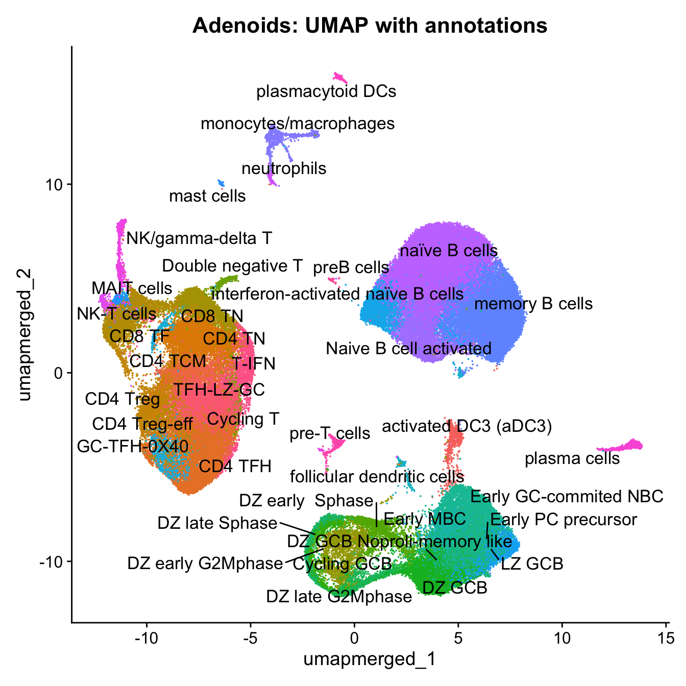
Save Final SEU object ( All cells)
out3 <- here("output",
            "RDS", "AllBatches_Final_Clusters_SEUs",
             paste0("G000231_Neeland_",tissue,".final_clusters.SEU.rds"))

if (!file.exists(out3)) {
  saveRDS(merged, file = out3)
}
Session Info
sessioninfo::session_info()─ Session info ───────────────────────────────────────────────────────────────
setting value
version R version 4.3.2 (2023-10-31)
os macOS Sonoma 14.6.1
system aarch64, darwin20
ui X11
language (EN)
collate en_US.UTF-8
ctype en_US.UTF-8
tz Australia/Melbourne
date 2024-09-23
pandoc 3.1.1 @ /Users/dixitgunjan/Desktop/RStudio.app/Contents/Resources/app/quarto/bin/tools/ (via rmarkdown)
─ Packages ───────────────────────────────────────────────────────────────────
package * version date (UTC) lib source
abind 1.4-5 2016-07-21 [1] CRAN (R 4.3.0)
AnnotationDbi * 1.64.1 2023-11-02 [1] Bioconductor
backports 1.4.1 2021-12-13 [1] CRAN (R 4.3.0)
beeswarm 0.4.0 2021-06-01 [1] CRAN (R 4.3.0)
Biobase * 2.62.0 2023-10-26 [1] Bioconductor
BiocGenerics * 0.48.1 2023-11-02 [1] Bioconductor
BiocManager 1.30.22 2023-08-08 [1] CRAN (R 4.3.0)
BiocStyle * 2.30.0 2023-10-26 [1] Bioconductor
Biostrings 2.70.2 2024-01-30 [1] Bioconductor 3.18 (R 4.3.2)
bit 4.0.5 2022-11-15 [1] CRAN (R 4.3.0)
bit64 4.0.5 2020-08-30 [1] CRAN (R 4.3.0)
bitops 1.0-7 2021-04-24 [1] CRAN (R 4.3.0)
blob 1.2.4 2023-03-17 [1] CRAN (R 4.3.0)
bslib 0.6.1 2023-11-28 [1] CRAN (R 4.3.1)
cachem 1.0.8 2023-05-01 [1] CRAN (R 4.3.0)
callr 3.7.5 2024-02-19 [1] CRAN (R 4.3.1)
cellranger 1.1.0 2016-07-27 [1] CRAN (R 4.3.0)
checkmate 2.3.1 2023-12-04 [1] CRAN (R 4.3.1)
cli 3.6.2 2023-12-11 [1] CRAN (R 4.3.1)
cluster 2.1.6 2023-12-01 [1] CRAN (R 4.3.1)
clustree * 0.5.1 2023-11-05 [1] CRAN (R 4.3.1)
codetools 0.2-19 2023-02-01 [1] CRAN (R 4.3.2)
colorspace 2.1-0 2023-01-23 [1] CRAN (R 4.3.0)
cowplot 1.1.3 2024-01-22 [1] CRAN (R 4.3.1)
crayon 1.5.2 2022-09-29 [1] CRAN (R 4.3.0)
data.table * 1.15.0 2024-01-30 [1] CRAN (R 4.3.1)
DBI 1.2.2 2024-02-16 [1] CRAN (R 4.3.1)
DelayedArray 0.28.0 2023-11-06 [1] Bioconductor
deldir 2.0-2 2023-11-23 [1] CRAN (R 4.3.1)
digest 0.6.34 2024-01-11 [1] CRAN (R 4.3.1)
dotCall64 1.1-1 2023-11-28 [1] CRAN (R 4.3.1)
dplyr * 1.1.4 2023-11-17 [1] CRAN (R 4.3.1)
edgeR * 4.0.16 2024-02-20 [1] Bioconductor 3.18 (R 4.3.2)
ellipsis 0.3.2 2021-04-29 [1] CRAN (R 4.3.0)
evaluate 0.23 2023-11-01 [1] CRAN (R 4.3.1)
fansi 1.0.6 2023-12-08 [1] CRAN (R 4.3.1)
farver 2.1.1 2022-07-06 [1] CRAN (R 4.3.0)
fastDummies 1.7.3 2023-07-06 [1] CRAN (R 4.3.0)
fastmap 1.1.1 2023-02-24 [1] CRAN (R 4.3.0)
fitdistrplus 1.1-11 2023-04-25 [1] CRAN (R 4.3.0)
forcats * 1.0.0 2023-01-29 [1] CRAN (R 4.3.0)
fs 1.6.3 2023-07-20 [1] CRAN (R 4.3.0)
future 1.33.1 2023-12-22 [1] CRAN (R 4.3.1)
future.apply 1.11.1 2023-12-21 [1] CRAN (R 4.3.1)
generics 0.1.3 2022-07-05 [1] CRAN (R 4.3.0)
GenomeInfoDb 1.38.6 2024-02-10 [1] Bioconductor 3.18 (R 4.3.2)
GenomeInfoDbData 1.2.11 2024-02-27 [1] Bioconductor
GenomicRanges 1.54.1 2023-10-30 [1] Bioconductor
getPass 0.2-4 2023-12-10 [1] CRAN (R 4.3.1)
ggbeeswarm 0.7.2 2023-04-29 [1] CRAN (R 4.3.0)
ggforce 0.4.2 2024-02-19 [1] CRAN (R 4.3.1)
ggplot2 * 3.5.0 2024-02-23 [1] CRAN (R 4.3.1)
ggraph * 2.1.0 2022-10-09 [1] CRAN (R 4.3.0)
ggrastr 1.0.2 2023-06-01 [1] CRAN (R 4.3.0)
ggrepel 0.9.5 2024-01-10 [1] CRAN (R 4.3.1)
ggridges 0.5.6 2024-01-23 [1] CRAN (R 4.3.1)
git2r 0.33.0 2023-11-26 [1] CRAN (R 4.3.1)
globals 0.16.2 2022-11-21 [1] CRAN (R 4.3.0)
glue * 1.7.0 2024-01-09 [1] CRAN (R 4.3.1)
goftest 1.2-3 2021-10-07 [1] CRAN (R 4.3.0)
graphlayouts 1.1.0 2024-01-19 [1] CRAN (R 4.3.1)
gridExtra 2.3 2017-09-09 [1] CRAN (R 4.3.0)
gtable 0.3.4 2023-08-21 [1] CRAN (R 4.3.0)
here * 1.0.1 2020-12-13 [1] CRAN (R 4.3.0)
highr 0.10 2022-12-22 [1] CRAN (R 4.3.0)
hms 1.1.3 2023-03-21 [1] CRAN (R 4.3.0)
htmltools 0.5.7 2023-11-03 [1] CRAN (R 4.3.1)
htmlwidgets 1.6.4 2023-12-06 [1] CRAN (R 4.3.1)
httpuv 1.6.14 2024-01-26 [1] CRAN (R 4.3.1)
httr 1.4.7 2023-08-15 [1] CRAN (R 4.3.0)
ica 1.0-3 2022-07-08 [1] CRAN (R 4.3.0)
igraph 2.0.2 2024-02-17 [1] CRAN (R 4.3.1)
IRanges * 2.36.0 2023-10-26 [1] Bioconductor
irlba 2.3.5.1 2022-10-03 [1] CRAN (R 4.3.2)
jquerylib 0.1.4 2021-04-26 [1] CRAN (R 4.3.0)
jsonlite 1.8.8 2023-12-04 [1] CRAN (R 4.3.1)
kableExtra * 1.4.0 2024-01-24 [1] CRAN (R 4.3.1)
KEGGREST 1.42.0 2023-10-26 [1] Bioconductor
KernSmooth 2.23-22 2023-07-10 [1] CRAN (R 4.3.2)
knitr 1.45 2023-10-30 [1] CRAN (R 4.3.1)
labeling 0.4.3 2023-08-29 [1] CRAN (R 4.3.0)
later 1.3.2 2023-12-06 [1] CRAN (R 4.3.1)
lattice 0.22-5 2023-10-24 [1] CRAN (R 4.3.1)
lazyeval 0.2.2 2019-03-15 [1] CRAN (R 4.3.0)
leiden 0.4.3.1 2023-11-17 [1] CRAN (R 4.3.1)
lifecycle 1.0.4 2023-11-07 [1] CRAN (R 4.3.1)
limma * 3.58.1 2023-11-02 [1] Bioconductor
listenv 0.9.1 2024-01-29 [1] CRAN (R 4.3.1)
lmtest 0.9-40 2022-03-21 [1] CRAN (R 4.3.0)
locfit 1.5-9.8 2023-06-11 [1] CRAN (R 4.3.0)
lubridate * 1.9.3 2023-09-27 [1] CRAN (R 4.3.1)
magrittr 2.0.3 2022-03-30 [1] CRAN (R 4.3.0)
MASS 7.3-60.0.1 2024-01-13 [1] CRAN (R 4.3.1)
Matrix 1.6-5 2024-01-11 [1] CRAN (R 4.3.1)
MatrixGenerics 1.14.0 2023-10-26 [1] Bioconductor
matrixStats 1.2.0 2023-12-11 [1] CRAN (R 4.3.1)
memoise 2.0.1 2021-11-26 [1] CRAN (R 4.3.0)
mime 0.12 2021-09-28 [1] CRAN (R 4.3.0)
miniUI 0.1.1.1 2018-05-18 [1] CRAN (R 4.3.0)
munsell 0.5.0 2018-06-12 [1] CRAN (R 4.3.0)
nlme 3.1-164 2023-11-27 [1] CRAN (R 4.3.1)
org.Hs.eg.db * 3.18.0 2024-02-27 [1] Bioconductor
paletteer 1.6.0 2024-01-21 [1] CRAN (R 4.3.1)
parallelly 1.37.0 2024-02-14 [1] CRAN (R 4.3.1)
patchwork * 1.2.0 2024-01-08 [1] CRAN (R 4.3.1)
pbapply 1.7-2 2023-06-27 [1] CRAN (R 4.3.0)
pillar 1.9.0 2023-03-22 [1] CRAN (R 4.3.0)
pkgconfig 2.0.3 2019-09-22 [1] CRAN (R 4.3.0)
plotly 4.10.4 2024-01-13 [1] CRAN (R 4.3.1)
plyr 1.8.9 2023-10-02 [1] CRAN (R 4.3.1)
png 0.1-8 2022-11-29 [1] CRAN (R 4.3.0)
polyclip 1.10-6 2023-09-27 [1] CRAN (R 4.3.1)
presto 1.0.0 2024-02-27 [1] Github (immunogenomics/presto@31dc97f)
prismatic 1.1.1 2022-08-15 [1] CRAN (R 4.3.0)
processx 3.8.3 2023-12-10 [1] CRAN (R 4.3.1)
progressr 0.14.0 2023-08-10 [1] CRAN (R 4.3.0)
promises 1.2.1 2023-08-10 [1] CRAN (R 4.3.0)
ps 1.7.6 2024-01-18 [1] CRAN (R 4.3.1)
purrr * 1.0.2 2023-08-10 [1] CRAN (R 4.3.0)
R6 2.5.1 2021-08-19 [1] CRAN (R 4.3.0)
RANN 2.6.1 2019-01-08 [1] CRAN (R 4.3.0)
RColorBrewer * 1.1-3 2022-04-03 [1] CRAN (R 4.3.0)
Rcpp 1.0.12 2024-01-09 [1] CRAN (R 4.3.1)
RcppAnnoy 0.0.22 2024-01-23 [1] CRAN (R 4.3.1)
RcppHNSW 0.6.0 2024-02-04 [1] CRAN (R 4.3.1)
RCurl 1.98-1.14 2024-01-09 [1] CRAN (R 4.3.1)
readr * 2.1.5 2024-01-10 [1] CRAN (R 4.3.1)
readxl * 1.4.3 2023-07-06 [1] CRAN (R 4.3.0)
rematch2 2.1.2 2020-05-01 [1] CRAN (R 4.3.0)
reshape2 1.4.4 2020-04-09 [1] CRAN (R 4.3.0)
reticulate 1.35.0 2024-01-31 [1] CRAN (R 4.3.1)
rlang 1.1.3 2024-01-10 [1] CRAN (R 4.3.1)
rmarkdown 2.25 2023-09-18 [1] CRAN (R 4.3.1)
ROCR 1.0-11 2020-05-02 [1] CRAN (R 4.3.0)
rprojroot 2.0.4 2023-11-05 [1] CRAN (R 4.3.1)
RSpectra 0.16-1 2022-04-24 [1] CRAN (R 4.3.0)
RSQLite 2.3.5 2024-01-21 [1] CRAN (R 4.3.1)
rstudioapi 0.15.0 2023-07-07 [1] CRAN (R 4.3.0)
Rtsne 0.17 2023-12-07 [1] CRAN (R 4.3.1)
S4Arrays 1.2.0 2023-10-26 [1] Bioconductor
S4Vectors * 0.40.2 2023-11-25 [1] Bioconductor 3.18 (R 4.3.2)
sass 0.4.8 2023-12-06 [1] CRAN (R 4.3.1)
scales 1.3.0 2023-11-28 [1] CRAN (R 4.3.1)
scattermore 1.2 2023-06-12 [1] CRAN (R 4.3.0)
sctransform 0.4.1 2023-10-19 [1] CRAN (R 4.3.1)
sessioninfo 1.2.2 2021-12-06 [1] CRAN (R 4.3.0)
Seurat * 5.0.1.9009 2024-02-28 [1] Github (satijalab/seurat@6a3ef5e)
SeuratObject * 5.0.1 2023-11-17 [1] CRAN (R 4.3.1)
shiny 1.8.0 2023-11-17 [1] CRAN (R 4.3.1)
SingleCellExperiment 1.24.0 2023-11-06 [1] Bioconductor
sp * 2.1-3 2024-01-30 [1] CRAN (R 4.3.1)
spam 2.10-0 2023-10-23 [1] CRAN (R 4.3.1)
SparseArray 1.2.4 2024-02-10 [1] Bioconductor 3.18 (R 4.3.2)
spatstat.data 3.0-4 2024-01-15 [1] CRAN (R 4.3.1)
spatstat.explore 3.2-6 2024-02-01 [1] CRAN (R 4.3.1)
spatstat.geom 3.2-8 2024-01-26 [1] CRAN (R 4.3.1)
spatstat.random 3.2-2 2023-11-29 [1] CRAN (R 4.3.1)
spatstat.sparse 3.0-3 2023-10-24 [1] CRAN (R 4.3.1)
spatstat.utils 3.0-4 2023-10-24 [1] CRAN (R 4.3.1)
speckle * 1.2.0 2023-10-26 [1] Bioconductor
statmod 1.5.0 2023-01-06 [1] CRAN (R 4.3.0)
stringi 1.8.3 2023-12-11 [1] CRAN (R 4.3.1)
stringr * 1.5.1 2023-11-14 [1] CRAN (R 4.3.1)
SummarizedExperiment 1.32.0 2023-11-06 [1] Bioconductor
survival 3.5-8 2024-02-14 [1] CRAN (R 4.3.1)
svglite 2.1.3 2023-12-08 [1] CRAN (R 4.3.1)
systemfonts 1.0.5 2023-10-09 [1] CRAN (R 4.3.1)
tensor 1.5 2012-05-05 [1] CRAN (R 4.3.0)
tibble * 3.2.1 2023-03-20 [1] CRAN (R 4.3.0)
tidygraph 1.3.1 2024-01-30 [1] CRAN (R 4.3.1)
tidyr * 1.3.1 2024-01-24 [1] CRAN (R 4.3.1)
tidyselect 1.2.0 2022-10-10 [1] CRAN (R 4.3.0)
tidyverse * 2.0.0 2023-02-22 [1] CRAN (R 4.3.0)
timechange 0.3.0 2024-01-18 [1] CRAN (R 4.3.1)
tweenr 2.0.3 2024-02-26 [1] CRAN (R 4.3.1)
tzdb 0.4.0 2023-05-12 [1] CRAN (R 4.3.0)
utf8 1.2.4 2023-10-22 [1] CRAN (R 4.3.1)
uwot 0.1.16 2023-06-29 [1] CRAN (R 4.3.0)
vctrs 0.6.5 2023-12-01 [1] CRAN (R 4.3.1)
vipor 0.4.7 2023-12-18 [1] CRAN (R 4.3.1)
viridis 0.6.5 2024-01-29 [1] CRAN (R 4.3.1)
viridisLite 0.4.2 2023-05-02 [1] CRAN (R 4.3.0)
whisker 0.4.1 2022-12-05 [1] CRAN (R 4.3.0)
withr 3.0.0 2024-01-16 [1] CRAN (R 4.3.1)
workflowr * 1.7.1 2023-08-23 [1] CRAN (R 4.3.0)
xfun 0.42 2024-02-08 [1] CRAN (R 4.3.1)
xml2 1.3.6 2023-12-04 [1] CRAN (R 4.3.1)
xtable 1.8-4 2019-04-21 [1] CRAN (R 4.3.0)
XVector 0.42.0 2023-10-26 [1] Bioconductor
yaml 2.3.8 2023-12-11 [1] CRAN (R 4.3.1)
zlibbioc 1.48.0 2023-10-26 [1] Bioconductor
zoo 1.8-12 2023-04-13 [1] CRAN (R 4.3.0)
[1] /Library/Frameworks/R.framework/Versions/4.3-arm64/Resources/library
──────────────────────────────────────────────────────────────────────────────
sessionInfo()R version 4.3.2 (2023-10-31)
Platform: aarch64-apple-darwin20 (64-bit)
Running under: macOS Sonoma 14.6.1
Matrix products: default
BLAS: /Library/Frameworks/R.framework/Versions/4.3-arm64/Resources/lib/libRblas.0.dylib
LAPACK: /Library/Frameworks/R.framework/Versions/4.3-arm64/Resources/lib/libRlapack.dylib; LAPACK version 3.11.0
locale:
[1] en_US.UTF-8/en_US.UTF-8/en_US.UTF-8/C/en_US.UTF-8/en_US.UTF-8
time zone: Australia/Melbourne
tzcode source: internal
attached base packages:
[1] stats4 stats graphics grDevices utils datasets methods
[8] base
other attached packages:
[1] readxl_1.4.3 org.Hs.eg.db_3.18.0 AnnotationDbi_1.64.1
[4] IRanges_2.36.0 S4Vectors_0.40.2 Biobase_2.62.0
[7] BiocGenerics_0.48.1 speckle_1.2.0 edgeR_4.0.16
[10] limma_3.58.1 patchwork_1.2.0 data.table_1.15.0
[13] RColorBrewer_1.1-3 kableExtra_1.4.0 clustree_0.5.1
[16] ggraph_2.1.0 Seurat_5.0.1.9009 SeuratObject_5.0.1
[19] sp_2.1-3 glue_1.7.0 here_1.0.1
[22] lubridate_1.9.3 forcats_1.0.0 stringr_1.5.1
[25] dplyr_1.1.4 purrr_1.0.2 readr_2.1.5
[28] tidyr_1.3.1 tibble_3.2.1 ggplot2_3.5.0
[31] tidyverse_2.0.0 BiocStyle_2.30.0 workflowr_1.7.1
loaded via a namespace (and not attached):
[1] fs_1.6.3 matrixStats_1.2.0
[3] spatstat.sparse_3.0-3 bitops_1.0-7
[5] httr_1.4.7 tools_4.3.2
[7] sctransform_0.4.1 backports_1.4.1
[9] utf8_1.2.4 R6_2.5.1
[11] lazyeval_0.2.2 uwot_0.1.16
[13] withr_3.0.0 gridExtra_2.3
[15] progressr_0.14.0 cli_3.6.2
[17] spatstat.explore_3.2-6 fastDummies_1.7.3
[19] prismatic_1.1.1 labeling_0.4.3
[21] sass_0.4.8 spatstat.data_3.0-4
[23] ggridges_0.5.6 pbapply_1.7-2
[25] systemfonts_1.0.5 svglite_2.1.3
[27] sessioninfo_1.2.2 parallelly_1.37.0
[29] rstudioapi_0.15.0 RSQLite_2.3.5
[31] generics_0.1.3 ica_1.0-3
[33] spatstat.random_3.2-2 Matrix_1.6-5
[35] ggbeeswarm_0.7.2 fansi_1.0.6
[37] abind_1.4-5 lifecycle_1.0.4
[39] whisker_0.4.1 yaml_2.3.8
[41] SummarizedExperiment_1.32.0 SparseArray_1.2.4
[43] Rtsne_0.17 paletteer_1.6.0
[45] grid_4.3.2 blob_1.2.4
[47] promises_1.2.1 crayon_1.5.2
[49] miniUI_0.1.1.1 lattice_0.22-5
[51] cowplot_1.1.3 KEGGREST_1.42.0
[53] pillar_1.9.0 knitr_1.45
[55] GenomicRanges_1.54.1 future.apply_1.11.1
[57] codetools_0.2-19 leiden_0.4.3.1
[59] getPass_0.2-4 vctrs_0.6.5
[61] png_0.1-8 spam_2.10-0
[63] cellranger_1.1.0 gtable_0.3.4
[65] rematch2_2.1.2 cachem_1.0.8
[67] xfun_0.42 S4Arrays_1.2.0
[69] mime_0.12 tidygraph_1.3.1
[71] survival_3.5-8 SingleCellExperiment_1.24.0
[73] statmod_1.5.0 ellipsis_0.3.2
[75] fitdistrplus_1.1-11 ROCR_1.0-11
[77] nlme_3.1-164 bit64_4.0.5
[79] RcppAnnoy_0.0.22 GenomeInfoDb_1.38.6
[81] rprojroot_2.0.4 bslib_0.6.1
[83] irlba_2.3.5.1 vipor_0.4.7
[85] KernSmooth_2.23-22 colorspace_2.1-0
[87] DBI_1.2.2 ggrastr_1.0.2
[89] tidyselect_1.2.0 processx_3.8.3
[91] bit_4.0.5 compiler_4.3.2
[93] git2r_0.33.0 xml2_1.3.6
[95] DelayedArray_0.28.0 plotly_4.10.4
[97] checkmate_2.3.1 scales_1.3.0
[99] lmtest_0.9-40 callr_3.7.5
[101] digest_0.6.34 goftest_1.2-3
[103] spatstat.utils_3.0-4 presto_1.0.0
[105] rmarkdown_2.25 XVector_0.42.0
[107] htmltools_0.5.7 pkgconfig_2.0.3
[109] MatrixGenerics_1.14.0 highr_0.10
[111] fastmap_1.1.1 rlang_1.1.3
[113] htmlwidgets_1.6.4 shiny_1.8.0
[115] farver_2.1.1 jquerylib_0.1.4
[117] zoo_1.8-12 jsonlite_1.8.8
[119] RCurl_1.98-1.14 magrittr_2.0.3
[121] GenomeInfoDbData_1.2.11 dotCall64_1.1-1
[123] munsell_0.5.0 Rcpp_1.0.12
[125] viridis_0.6.5 reticulate_1.35.0
[127] stringi_1.8.3 zlibbioc_1.48.0
[129] MASS_7.3-60.0.1 plyr_1.8.9
[131] parallel_4.3.2 listenv_0.9.1
[133] ggrepel_0.9.5 deldir_2.0-2
[135] Biostrings_2.70.2 graphlayouts_1.1.0
[137] splines_4.3.2 tensor_1.5
[139] hms_1.1.3 locfit_1.5-9.8
[141] ps_1.7.6 igraph_2.0.2
[143] spatstat.geom_3.2-8 RcppHNSW_0.6.0
[145] reshape2_1.4.4 evaluate_0.23
[147] BiocManager_1.30.22 tzdb_0.4.0
[149] tweenr_2.0.3 httpuv_1.6.14
[151] RANN_2.6.1 polyclip_1.10-6
[153] future_1.33.1 scattermore_1.2
[155] ggforce_0.4.2 xtable_1.8-4
[157] RSpectra_0.16-1 later_1.3.2
[159] viridisLite_0.4.2 beeswarm_0.4.0
[161] memoise_2.0.1 cluster_2.1.6
[163] timechange_0.3.0 globals_0.16.2