Subclustering: Tonsils
Unsupervised Clustering of Broad cell labels
Gunjan Dixit
September 23, 2024
Last updated: 2024-09-23
Checks: 6 1
Knit directory: paed-airway-allTissues/
This reproducible R Markdown analysis was created with workflowr (version 1.7.1). The Checks tab describes the reproducibility checks that were applied when the results were created. The Past versions tab lists the development history.
The R Markdown is untracked by Git. To know which version of the R
Markdown file created these results, you’ll want to first commit it to
the Git repo. If you’re still working on the analysis, you can ignore
this warning. When you’re finished, you can run
wflow_publish to commit the R Markdown file and build the
HTML.
Great job! The global environment was empty. Objects defined in the global environment can affect the analysis in your R Markdown file in unknown ways. For reproduciblity it’s best to always run the code in an empty environment.
The command set.seed(20230811) was run prior to running
the code in the R Markdown file. Setting a seed ensures that any results
that rely on randomness, e.g. subsampling or permutations, are
reproducible.
Great job! Recording the operating system, R version, and package versions is critical for reproducibility.
Nice! There were no cached chunks for this analysis, so you can be confident that you successfully produced the results during this run.
Great job! Using relative paths to the files within your workflowr project makes it easier to run your code on other machines.
Great! You are using Git for version control. Tracking code development and connecting the code version to the results is critical for reproducibility.
The results in this page were generated with repository version 901215e. See the Past versions tab to see a history of the changes made to the R Markdown and HTML files.
Note that you need to be careful to ensure that all relevant files for
the analysis have been committed to Git prior to generating the results
(you can use wflow_publish or
wflow_git_commit). workflowr only checks the R Markdown
file, but you know if there are other scripts or data files that it
depends on. Below is the status of the Git repository when the results
were generated:
Ignored files:
    Ignored:    .DS_Store
    Ignored:    .RData
    Ignored:    .Rhistory
    Ignored:    .Rproj.user/
    Ignored:    analysis/.DS_Store
    Ignored:    data/.DS_Store
    Ignored:    data/RDS/
    Ignored:    output/.DS_Store
    Ignored:    output/CSV/.DS_Store
    Ignored:    output/G000231_Neeland_batch1/
    Ignored:    output/G000231_Neeland_batch2_1/
    Ignored:    output/G000231_Neeland_batch2_2/
    Ignored:    output/G000231_Neeland_batch3/
    Ignored:    output/G000231_Neeland_batch4/
    Ignored:    output/G000231_Neeland_batch5/
    Ignored:    output/G000231_Neeland_batch9_1/
    Ignored:    output/RDS/
    Ignored:    output/plots/

Untracked files:
    Untracked:  Adenoids_Bcell_subset_proportions_Age.pdf
    Untracked:  Adenoids_Tcell_subset_proportions_Age.pdf
    Untracked:  Adenoids_cell_type_proportions_Age.pdf
    Untracked:  Age_proportions_Adenoids.pdf
    Untracked:  Age_proportions_Bronchial_brushings.pdf
    Untracked:  Age_proportions_Nasal_brushings.pdf
    Untracked:  Age_proportions_Tonsils.pdf
    Untracked:  BAL_Tcell_propeller.xlsx
    Untracked:  BAL_propeller.xlsx
    Untracked:  BB_Tcell_propeller.xlsx
    Untracked:  BB_propeller.xlsx
    Untracked:  NB_Tcell_propeller.xlsx
    Untracked:  NB_propeller.csv
    Untracked:  NB_propeller.pdf
    Untracked:  NB_propeller.xlsx
    Untracked:  Tonsils_cell_type_proportions.jpg
    Untracked:  Tonsils_cell_type_proportions.pdf
    Untracked:  Tonsils_cell_type_proportions.png
    Untracked:  Tonsils_cell_type_proportions_Age.pdf
    Untracked:  analysis/03_Batch_Integration.Rmd
    Untracked:  analysis/Age_modelling_Adenoids.Rmd
    Untracked:  analysis/Age_modelling_Bronchial_Brushings.Rmd
    Untracked:  analysis/Age_modelling_Nasal_Brushings.Rmd
    Untracked:  analysis/Age_modelling_Tonsils.Rmd
    Untracked:  analysis/Age_proportions.Rmd
    Untracked:  analysis/Age_proportions_AllBatches.Rmd
    Untracked:  analysis/BAL_without_DecontX.Rmd
    Untracked:  analysis/Batch_Integration_&_Downstream_analysis.Rmd
    Untracked:  analysis/Batch_correction_&_Downstream.Rmd
    Untracked:  analysis/Boxplot_Adenoids.pdf
    Untracked:  analysis/Boxplot_BAL.pdf
    Untracked:  analysis/Boxplot_Bronchial_brushings.pdf
    Untracked:  analysis/Boxplot_Nasal_brushings.pdf
    Untracked:  analysis/Boxplot_Tonsils.pdf
    Untracked:  analysis/Cell_cycle_regression.Rmd
    Untracked:  analysis/Master_metadata.Rmd
    Untracked:  analysis/Preprocessing_Batch1_Nasal_brushings.Rmd
    Untracked:  analysis/Preprocessing_Batch2_Tonsils.Rmd
    Untracked:  analysis/Preprocessing_Batch3_Adenoids.Rmd
    Untracked:  analysis/Preprocessing_Batch4_Bronchial_brushings.Rmd
    Untracked:  analysis/Preprocessing_Batch5_Nasal_brushings.Rmd
    Untracked:  analysis/Preprocessing_Batch6_BAL.Rmd
    Untracked:  analysis/Preprocessing_Batch7_Bronchial_brushings.Rmd
    Untracked:  analysis/Preprocessing_Batch8_Adenoids.Rmd
    Untracked:  analysis/Preprocessing_Batch9_Tonsils.Rmd
    Untracked:  analysis/Subclustering_Adenoids.Rmd
    Untracked:  analysis/Subclustering_Nasal_brushings.Rmd
    Untracked:  analysis/Subclustering_Tonsils.Rmd
    Untracked:  analysis/TonsilsVsAdenoids.Rmd
    Untracked:  analysis/boxplot_proportions_Adenoids.pdf
    Untracked:  analysis/boxplot_proportions_BAL.pdf
    Untracked:  analysis/boxplot_proportions_Bronchial_brushings.pdf
    Untracked:  analysis/boxplot_proportions_Nasal_brushings.pdf
    Untracked:  analysis/boxplot_proportions_Tonsils.pdf
    Untracked:  analysis/boxplot_proportions__broad_l2Adenoids.pdf
    Untracked:  analysis/boxplot_proportions__broad_l2BAL.pdf
    Untracked:  analysis/boxplot_proportions__broad_l2Bronchial_brushings.pdf
    Untracked:  analysis/boxplot_proportions__broad_l2Nasal_brushings.pdf
    Untracked:  analysis/boxplot_proportions__broad_l2Tonsils.pdf
    Untracked:  analysis/cell_cycle_regression.R
    Untracked:  analysis/test.Rmd
    Untracked:  analysis/testing_age_all.Rmd
    Untracked:  cell_proportions_overview.png
    Untracked:  cell_type_proportions.pdf
    Untracked:  cell_type_proportions_enhanced.pdf
    Untracked:  cell_type_proportions_individual.pdf
    Untracked:  color_palette.rds
    Untracked:  color_palette_v2_level2.rds
    Untracked:  combined_metadata.rds
    Untracked:  data/Cell_labels_Mel/
    Untracked:  data/Cell_labels_Mel_v2/
    Untracked:  data/Cell_labels_modified_Gunjan/
    Untracked:  data/Hs.c2.cp.reactome.v7.1.entrez.rds
    Untracked:  data/Raw_feature_bc_matrix/
    Untracked:  data/celltypes_Mel_GD_v3.xlsx
    Untracked:  data/celltypes_Mel_GD_v4_no_dups.xlsx
    Untracked:  data/celltypes_Mel_modified.xlsx
    Untracked:  data/celltypes_Mel_v2.csv
    Untracked:  data/celltypes_Mel_v2.xlsx
    Untracked:  data/celltypes_Mel_v2_MN.xlsx
    Untracked:  data/celltypes_for_mel_MN.xlsx
    Untracked:  data/earlyAIR_sample_sheets_combined.xlsx
    Untracked:  output/CSV/All_tissues.propeller.xlsx
    Untracked:  output/CSV/Bronchial_brushings/
    Untracked:  output/CSV/Bronchial_brushings_Marker_gene_clusters.limmaTrendRNA_snn_res.0.4/
    Untracked:  output/CSV/G000231_Neeland_Adenoids.propeller.xlsx
    Untracked:  output/CSV/G000231_Neeland_Bronchial_brushings.propeller.xlsx
    Untracked:  output/CSV/G000231_Neeland_Nasal_brushings.propeller.xlsx
    Untracked:  output/CSV/G000231_Neeland_Tonsils.propeller.xlsx
    Untracked:  output/CSV/Nasal_brushings/

Unstaged changes:
    Deleted:    02_QC_exploratoryPlots.Rmd
    Deleted:    02_QC_exploratoryPlots.html
    Modified:   analysis/00_AllBatches_overview.Rmd
    Modified:   analysis/01_QC_emptyDrops.Rmd
    Modified:   analysis/02_QC_exploratoryPlots.Rmd
    Modified:   analysis/Adenoids.Rmd
    Modified:   analysis/Age_modeling.Rmd
    Modified:   analysis/AllBatches_QCExploratory.Rmd
    Modified:   analysis/BAL.Rmd
    Modified:   analysis/Bronchial_brushings.Rmd
    Modified:   analysis/Nasal_brushings.Rmd
    Modified:   analysis/Tonsils.Rmd
    Modified:   analysis/index.Rmd
    Modified:   output/CSV/BAL_Marker_gene_clusters.limmaTrendRNA_snn_res.0.4/REACTOME-cluster-limma-c0.csv
    Modified:   output/CSV/BAL_Marker_gene_clusters.limmaTrendRNA_snn_res.0.4/REACTOME-cluster-limma-c1.csv
    Modified:   output/CSV/BAL_Marker_gene_clusters.limmaTrendRNA_snn_res.0.4/REACTOME-cluster-limma-c10.csv
    Modified:   output/CSV/BAL_Marker_gene_clusters.limmaTrendRNA_snn_res.0.4/REACTOME-cluster-limma-c11.csv
    Modified:   output/CSV/BAL_Marker_gene_clusters.limmaTrendRNA_snn_res.0.4/REACTOME-cluster-limma-c12.csv
    Modified:   output/CSV/BAL_Marker_gene_clusters.limmaTrendRNA_snn_res.0.4/REACTOME-cluster-limma-c13.csv
    Modified:   output/CSV/BAL_Marker_gene_clusters.limmaTrendRNA_snn_res.0.4/REACTOME-cluster-limma-c14.csv
    Modified:   output/CSV/BAL_Marker_gene_clusters.limmaTrendRNA_snn_res.0.4/REACTOME-cluster-limma-c15.csv
    Modified:   output/CSV/BAL_Marker_gene_clusters.limmaTrendRNA_snn_res.0.4/REACTOME-cluster-limma-c16.csv
    Modified:   output/CSV/BAL_Marker_gene_clusters.limmaTrendRNA_snn_res.0.4/REACTOME-cluster-limma-c17.csv
    Modified:   output/CSV/BAL_Marker_gene_clusters.limmaTrendRNA_snn_res.0.4/REACTOME-cluster-limma-c2.csv
    Modified:   output/CSV/BAL_Marker_gene_clusters.limmaTrendRNA_snn_res.0.4/REACTOME-cluster-limma-c3.csv
    Modified:   output/CSV/BAL_Marker_gene_clusters.limmaTrendRNA_snn_res.0.4/REACTOME-cluster-limma-c4.csv
    Modified:   output/CSV/BAL_Marker_gene_clusters.limmaTrendRNA_snn_res.0.4/REACTOME-cluster-limma-c5.csv
    Modified:   output/CSV/BAL_Marker_gene_clusters.limmaTrendRNA_snn_res.0.4/REACTOME-cluster-limma-c6.csv
    Modified:   output/CSV/BAL_Marker_gene_clusters.limmaTrendRNA_snn_res.0.4/REACTOME-cluster-limma-c7.csv
    Modified:   output/CSV/BAL_Marker_gene_clusters.limmaTrendRNA_snn_res.0.4/REACTOME-cluster-limma-c8.csv
    Modified:   output/CSV/BAL_Marker_gene_clusters.limmaTrendRNA_snn_res.0.4/REACTOME-cluster-limma-c9.csv
    Modified:   output/CSV/BAL_Marker_gene_clusters.limmaTrendRNA_snn_res.0.4/up-cluster-limma-c0.csv
    Modified:   output/CSV/BAL_Marker_gene_clusters.limmaTrendRNA_snn_res.0.4/up-cluster-limma-c1.csv
    Modified:   output/CSV/BAL_Marker_gene_clusters.limmaTrendRNA_snn_res.0.4/up-cluster-limma-c10.csv
    Modified:   output/CSV/BAL_Marker_gene_clusters.limmaTrendRNA_snn_res.0.4/up-cluster-limma-c11.csv
    Modified:   output/CSV/BAL_Marker_gene_clusters.limmaTrendRNA_snn_res.0.4/up-cluster-limma-c12.csv
    Modified:   output/CSV/BAL_Marker_gene_clusters.limmaTrendRNA_snn_res.0.4/up-cluster-limma-c13.csv
    Modified:   output/CSV/BAL_Marker_gene_clusters.limmaTrendRNA_snn_res.0.4/up-cluster-limma-c14.csv
    Modified:   output/CSV/BAL_Marker_gene_clusters.limmaTrendRNA_snn_res.0.4/up-cluster-limma-c15.csv
    Modified:   output/CSV/BAL_Marker_gene_clusters.limmaTrendRNA_snn_res.0.4/up-cluster-limma-c16.csv
    Modified:   output/CSV/BAL_Marker_gene_clusters.limmaTrendRNA_snn_res.0.4/up-cluster-limma-c17.csv
    Modified:   output/CSV/BAL_Marker_gene_clusters.limmaTrendRNA_snn_res.0.4/up-cluster-limma-c2.csv
    Modified:   output/CSV/BAL_Marker_gene_clusters.limmaTrendRNA_snn_res.0.4/up-cluster-limma-c3.csv
    Modified:   output/CSV/BAL_Marker_gene_clusters.limmaTrendRNA_snn_res.0.4/up-cluster-limma-c4.csv
    Modified:   output/CSV/BAL_Marker_gene_clusters.limmaTrendRNA_snn_res.0.4/up-cluster-limma-c5.csv
    Modified:   output/CSV/BAL_Marker_gene_clusters.limmaTrendRNA_snn_res.0.4/up-cluster-limma-c6.csv
    Modified:   output/CSV/BAL_Marker_gene_clusters.limmaTrendRNA_snn_res.0.4/up-cluster-limma-c7.csv
    Modified:   output/CSV/BAL_Marker_gene_clusters.limmaTrendRNA_snn_res.0.4/up-cluster-limma-c8.csv
    Modified:   output/CSV/BAL_Marker_gene_clusters.limmaTrendRNA_snn_res.0.4/up-cluster-limma-c9.csv
Note that any generated files, e.g. HTML, png, CSS, etc., are not included in this status report because it is ok for generated content to have uncommitted changes.
There are no past versions. Publish this analysis with
wflow_publish() to start tracking its development.
Introduction
Load libraries
suppressPackageStartupMessages({
  library(BiocStyle)
  library(tidyverse)
  library(here)
  library(glue)
  library(dplyr)
  library(Seurat)
  library(clustree)
  library(kableExtra)
  library(RColorBrewer)
  library(data.table)
  library(ggplot2)
  library(patchwork)
  library(limma)
  library(edgeR)
  library(speckle)
  library(AnnotationDbi)
  library(org.Hs.eg.db)
  library(readxl)
})
Load Input data
Load merged object (batch corrected/integrated) for the tissue.
tissue <- "Tonsils"
out1 <- here("output",
            "RDS", "AllBatches_Clustering_SEUs",
             paste0("G000231_Neeland_",tissue,".Clusters.SEU.rds"))

merged_obj <- readRDS(out1)
merged_obj
An object of class Seurat
17566 features across 141705 samples within 1 assay
Active assay: RNA (17566 features, 2000 variable features)
3 layers present: data, counts, scale.data
4 dimensional reductions calculated: pca, umap.unintegrated, harmony, umap.harmonyReclustering T cell subtypes
Reclustering clusters 1, 4, 7, 8, 10, 17, 19, 20, 22
The marker genes for this reclustering can be found here-
Tonsils_Tcell_population_res.0.4
sub_clusters <- c(1, 4, 7, 8, 10, 17, 19, 20, 22)

idx <- which(merged_obj$cluster %in% sub_clusters)
paed_sub <- merged_obj[,idx]
paed_sub
An object of class Seurat
17566 features across 50340 samples within 1 assay
Active assay: RNA (17566 features, 2000 variable features)
3 layers present: data, counts, scale.data
4 dimensional reductions calculated: pca, umap.unintegrated, harmony, umap.harmony# Visualize the clustering results
DimPlot(paed_sub, reduction = "umap.harmony", group.by = "cluster", label = TRUE, label.size = 2.5, repel = TRUE, raster = FALSE )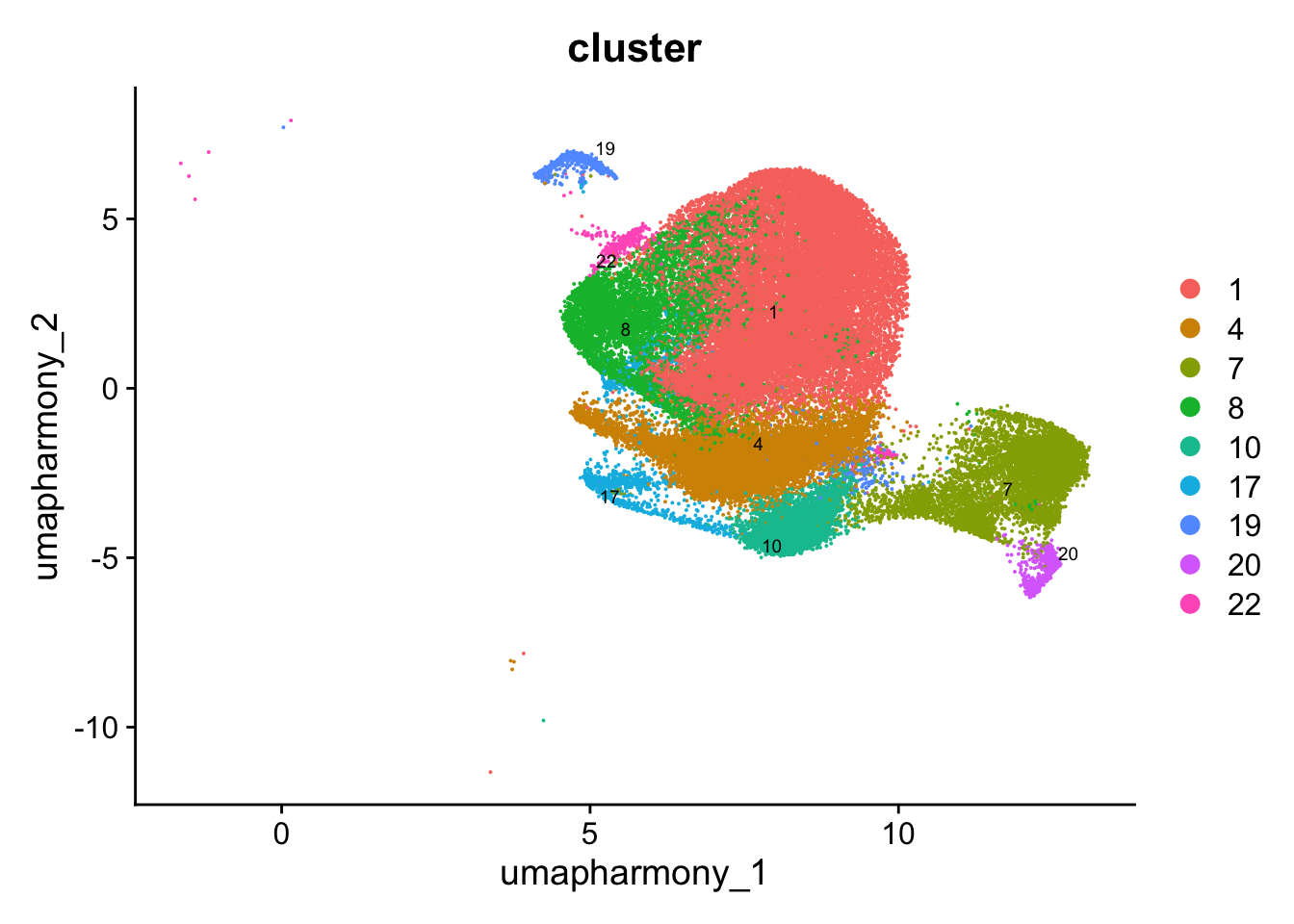
paed_sub <- paed_sub %>%
  NormalizeData() %>%
  FindVariableFeatures() %>%
  ScaleData() %>%
  RunPCA()
Normalizing layer: countsFinding variable features for layer countsCentering and scaling data matrixWarning: Different features in new layer data than already exists for
scale.dataPC_ 1
Positive: MAF, TOX2, PDCD1, CXCR5, TIGIT, POU2AF1, ICOS, IL21, SRGN, IKZF3
FAM43A, GNG4, ST8SIA1, TRIM8, RTP5, KIAA1324, SMCO4, BCL6, CTSB, TOX
ZNF703, TBC1D4, CD4, ITM2A, RNF19A, CTLA4, KCNK5, STK39, SARDH, RAB27A
Negative: KLF2, VIM, RASGRP2, TXNIP, SELL, EMP3, NELL2, CCR7, LEF1, RIPOR2
TMSB10, PLAC8, SAMHD1, S1PR1, KLRK1, PDE3B, IL7R, SAMD3, TRABD2A, CD55
CD96, NOG, PECAM1, CD8A, MGAT4A, FLT3LG, ITGA6, ITGB7, RASSF3, RASA3
PC_ 2
Positive: ACTN1, LEF1, CCR7, NOG, TRABD2A, LTB, CD40LG, LDHB, RASGRP2, CD4
SATB1, ITGA6, FHIT, MAL, NOSIP, OBSCN, EDAR, SELL, TMEM272, CSGALNACT1
PDK1, FKBP5, EPHX2, IL7R, SULT1B1, IL6R, AIF1, LRRN3, CDK5R1, PLAC8
Negative: NKG7, CST7, CCL5, GZMA, GZMK, CCR5, EOMES, CXCR6, KLRD1, PRF1
SLAMF7, CCL4, GNLY, PLEK, MYO1F, KLRK1, APOBEC3G, CTSW, IL2RB, AHNAK
FGR, FASLG, CLDND1, CXCR3, CD300A, PRR5L, KLRG1, ZEB2, HOPX, LAG3
PC_ 3
Positive: NKG7, CCL5, GZMK, EOMES, FCRL6, KLRK1, KLRG1, CXCR4, SLAMF7, AOAH
GZMA, CST7, CD8A, KLRD1, PLEK, KLRC4, CXCR5, TRGC2, DKK3, PTGDR
PRR5L, FGR, ITM2C, KLRC3, SPRY2, CCL4, CTSW, RTP5, ST8SIA1, CNIH3
Negative: COL5A3, RORA, CCND2, CTLA4, F5, IL2RA, GBP2, TMSB10, FOXP3, ZC3H12D
PRDM1, DUSP16, IL1R1, SLAMF1, IL1R2, ADTRP, LAG3, BCL2, TMEM173, PIM2
CCR7, TNFRSF1B, TNFRSF4, CD4, IRF4, CCR6, SAMHD1, LTB, ADAM19, FURIN
PC_ 4
Positive: KLRB1, RGS1, CXCR6, GPR183, PRDM1, MAF, CSF1, ADAM19, COL5A3, CCR4
PYHIN1, NABP1, CCR6, CCR5, PHTF2, ATP2B4, GLIPR1, KLF6, CD4, RORA
NBEAL2, FOXP3, IL1R2, SYNE2, PCDH1, DUSP1, SLAMF1, DUSP16, AHNAK, MAP3K5
Negative: LEF1, GNG4, NUCB2, ACTN1, PECAM1, MYB, KLRK1, CD55, MT-CO2, BACH2
RIPOR2, CXXC5, RIN3, NELL2, SPN, MT-CO3, MT-ND4L, MT-ND4, CTSW, MT-ATP6
TRABD2A, CD200, CD248, PKM, XXYLT1, ENO1, MT-CYB, HSP90AB1, DGKZ, PTPN14
PC_ 5
Positive: GNLY, SH2D1B, TYROBP, FCER1G, ATP8B4, ITGAX, KLRC1, NCAM1, KLRF1, ITGAM
NCR1, TRDC, HOPX, IL18RAP, KIT, XCL2, KLRD1, KLRB1, FES, KLRC3
IL7R, DLL1, ZBTB16, TLE1, SPTSSB, FGR, CTSW, TNFRSF18, ID2, DOCK5
Negative: GZMK, EOMES, PTPN3, GZMA, SLAMF7, DTHD1, CCR5, CD8A, CCL5, CD27
CST7, CAV1, CCL4, ANXA2, DKK3, FASLG, MYB, LYST, PRDM8, AGAP1
PECAM1, MPP1, SH2D1A, KLRG1, MT2A, PHLDA1, TIGIT, FABP5, CLDND1, PLEK paed_sub <- RunUMAP(paed_sub, dims = 1:30, reduction = "pca", reduction.name = "umap.new")Warning: The default method for RunUMAP has changed from calling Python UMAP via reticulate to the R-native UWOT using the cosine metric
To use Python UMAP via reticulate, set umap.method to 'umap-learn' and metric to 'correlation'
This message will be shown once per session21:15:30 UMAP embedding parameters a = 0.9922 b = 1.112Found more than one class "dist" in cache; using the first, from namespace 'spam'Also defined by 'BiocGenerics'21:15:30 Read 50340 rows and found 30 numeric columns21:15:30 Using Annoy for neighbor search, n_neighbors = 30Found more than one class "dist" in cache; using the first, from namespace 'spam'Also defined by 'BiocGenerics'21:15:30 Building Annoy index with metric = cosine, n_trees = 500% 10 20 30 40 50 60 70 80 90 100%[----|----|----|----|----|----|----|----|----|----|**************************************************|
21:15:32 Writing NN index file to temp file /var/folders/q8/kw1r78g12qn793xm7g0zvk94x2bh70/T//RtmpvL9Y3z/file397c10cbaf2
21:15:32 Searching Annoy index using 1 thread, search_k = 3000
21:15:42 Annoy recall = 100%
21:15:42 Commencing smooth kNN distance calibration using 1 thread with target n_neighbors = 30
21:15:43 Initializing from normalized Laplacian + noise (using RSpectra)
21:15:44 Commencing optimization for 200 epochs, with 2237560 positive edges
21:15:59 Optimization finishedmeta_data_columns <- colnames(paed_sub@meta.data)
columns_to_remove <- grep("^RNA_snn_res", meta_data_columns, value = TRUE)
paed_sub@meta.data <- paed_sub@meta.data[, !(colnames(paed_sub@meta.data) %in% columns_to_remove)]resolutions <- seq(0.1, 1, by = 0.1)
paed_sub <- FindNeighbors(paed_sub, dims = 1:30, reduction = "pca")Computing nearest neighbor graphComputing SNNpaed_sub <- FindClusters(paed_sub, resolution = resolutions )Modularity Optimizer version 1.3.0 by Ludo Waltman and Nees Jan van Eck
Number of nodes: 50340
Number of edges: 1519068
Running Louvain algorithm...
Maximum modularity in 10 random starts: 0.9527
Number of communities: 7
Elapsed time: 9 seconds
Modularity Optimizer version 1.3.0 by Ludo Waltman and Nees Jan van Eck
Number of nodes: 50340
Number of edges: 1519068
Running Louvain algorithm...
Maximum modularity in 10 random starts: 0.9315
Number of communities: 11
Elapsed time: 8 seconds
Modularity Optimizer version 1.3.0 by Ludo Waltman and Nees Jan van Eck
Number of nodes: 50340
Number of edges: 1519068
Running Louvain algorithm...
Maximum modularity in 10 random starts: 0.9186
Number of communities: 16
Elapsed time: 8 seconds
Modularity Optimizer version 1.3.0 by Ludo Waltman and Nees Jan van Eck
Number of nodes: 50340
Number of edges: 1519068
Running Louvain algorithm...
Maximum modularity in 10 random starts: 0.9075
Number of communities: 17
Elapsed time: 8 seconds
Modularity Optimizer version 1.3.0 by Ludo Waltman and Nees Jan van Eck
Number of nodes: 50340
Number of edges: 1519068
Running Louvain algorithm...
Maximum modularity in 10 random starts: 0.8975
Number of communities: 18
Elapsed time: 8 seconds
Modularity Optimizer version 1.3.0 by Ludo Waltman and Nees Jan van Eck
Number of nodes: 50340
Number of edges: 1519068
Running Louvain algorithm...
Maximum modularity in 10 random starts: 0.8895
Number of communities: 19
Elapsed time: 7 seconds
Modularity Optimizer version 1.3.0 by Ludo Waltman and Nees Jan van Eck
Number of nodes: 50340
Number of edges: 1519068
Running Louvain algorithm...
Maximum modularity in 10 random starts: 0.8819
Number of communities: 19
Elapsed time: 8 seconds
Modularity Optimizer version 1.3.0 by Ludo Waltman and Nees Jan van Eck
Number of nodes: 50340
Number of edges: 1519068
Running Louvain algorithm...
Maximum modularity in 10 random starts: 0.8746
Number of communities: 20
Elapsed time: 8 seconds
Modularity Optimizer version 1.3.0 by Ludo Waltman and Nees Jan van Eck
Number of nodes: 50340
Number of edges: 1519068
Running Louvain algorithm...
Maximum modularity in 10 random starts: 0.8670
Number of communities: 20
Elapsed time: 7 seconds
Modularity Optimizer version 1.3.0 by Ludo Waltman and Nees Jan van Eck
Number of nodes: 50340
Number of edges: 1519068
Running Louvain algorithm...
Maximum modularity in 10 random starts: 0.8599
Number of communities: 23
Elapsed time: 7 secondsclustree(paed_sub, prefix = "RNA_snn_res.")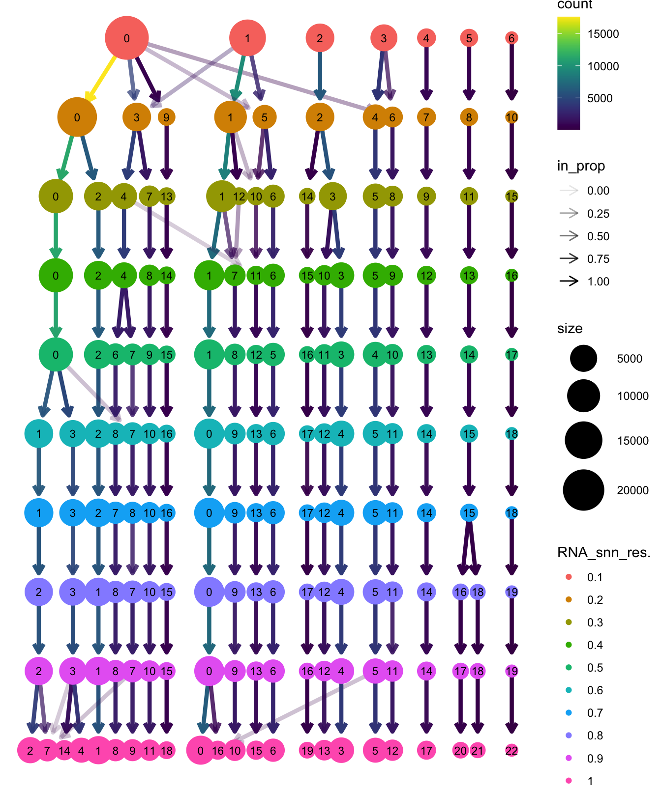
# Visualize the clustering results
DimPlot(paed_sub, group.by = "RNA_snn_res.0.4", reduction = "umap.new", label = TRUE, label.size = 2.5, repel = TRUE, raster = FALSE )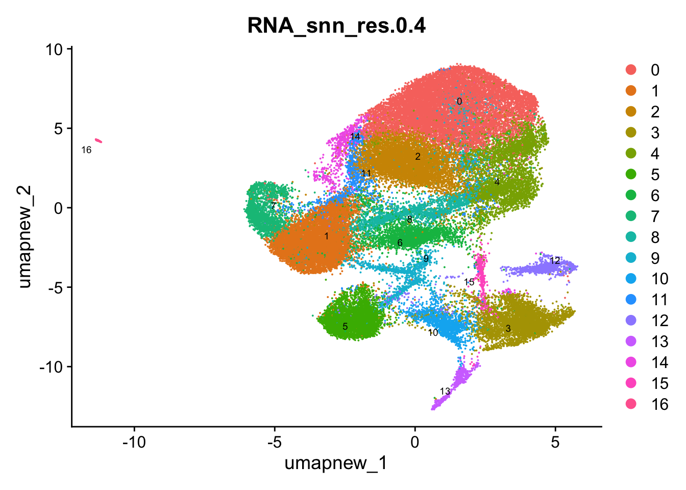
opt_res <- "RNA_snn_res.0.4"
n <- nlevels(paed_sub$RNA_snn_res.0.4)
paed_sub$RNA_snn_res.0.4 <- factor(paed_sub$RNA_snn_res.0.4, levels = seq(0,n-1))
paed_sub$seurat_clusters <- NULL
paed_sub$cluster <- paed_sub$RNA_snn_res.0.4
Idents(paed_sub) <- paed_sub$cluster
paed_sub.markers <- FindAllMarkers(paed_sub, only.pos = TRUE, min.pct = 0.25, logfc.threshold = 0.25)Calculating cluster 0Calculating cluster 1Calculating cluster 2Calculating cluster 3Calculating cluster 4Calculating cluster 5Calculating cluster 6Calculating cluster 7Calculating cluster 8Calculating cluster 9Calculating cluster 10Calculating cluster 11Calculating cluster 12Calculating cluster 13Calculating cluster 14Calculating cluster 15Calculating cluster 16paed_sub.markers %>%
group_by(cluster) %>% unique() %>%
top_n(n = 5, wt = avg_log2FC) -> top5
paed_sub.markers %>%
group_by(cluster) %>%
slice_head(n=1) %>%
pull(gene) -> best.wilcox.gene.per.cluster
best.wilcox.gene.per.cluster [1] "TOX2" "KLF2" "GPR183" "CCL5" "PRDM1" "CD8A" "KLF2" "LEF1"
[9] "FOXP3" "IFI44L" "KLRK1" "ZAP70" "GZMK" "TRDC" "ACTB" "NKG7"
[17] "DNTT" Feature plot shows the expression of top marker genes per cluster.
FeaturePlot(paed_sub,features=best.wilcox.gene.per.cluster, reduction = 'umap.new', raster = FALSE, ncol = 2, label = TRUE)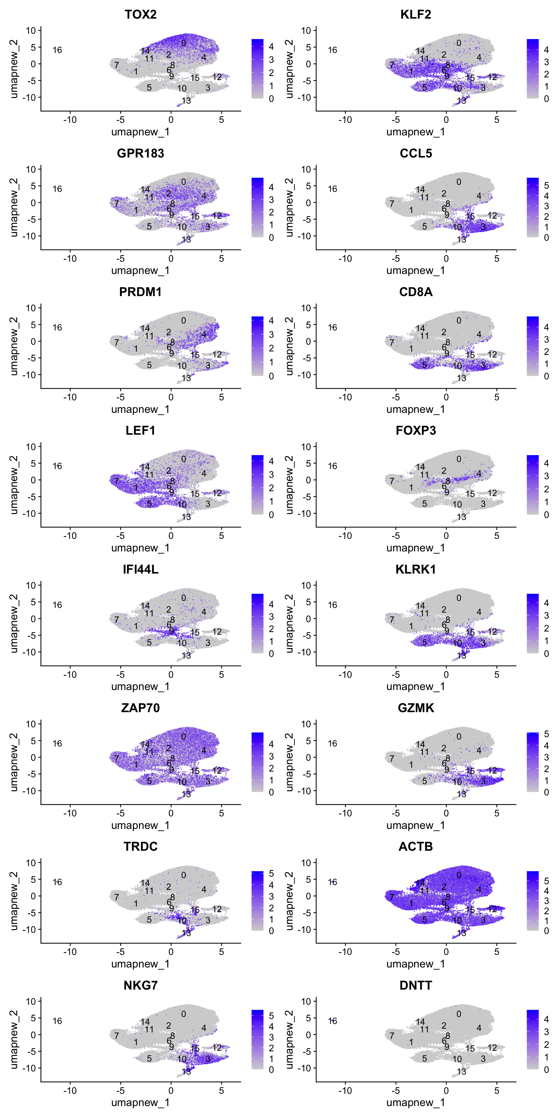
Top 10 marker genes from Seurat
## Seurat top markers
top10 <- paed_sub.markers %>%
    group_by(cluster) %>%
    top_n(n = 10, wt = avg_log2FC) %>%
    ungroup() %>%
    distinct(gene, .keep_all = TRUE) %>%
    arrange(cluster, desc(avg_log2FC))

cluster_colors <- paletteer::paletteer_d("pals::glasbey")[factor(top10$cluster)]

DotPlot(paed_sub,
        features = unique(top10$gene),
        group.by = opt_res,
        cols = c("azure1", "blueviolet"),
        dot.scale = 3, assay = "RNA") +
    RotatedAxis() +
    FontSize(y.text = 8, x.text = 12) +
    labs(y = element_blank(), x = element_blank()) +
    coord_flip() +
    theme(axis.text.y = element_text(color = cluster_colors)) +
    ggtitle("Top 10 marker genes per cluster (Seurat)")
Warning: Vectorized input to `element_text()` is not officially supported.
ℹ Results may be unexpected or may change in future versions of ggplot2.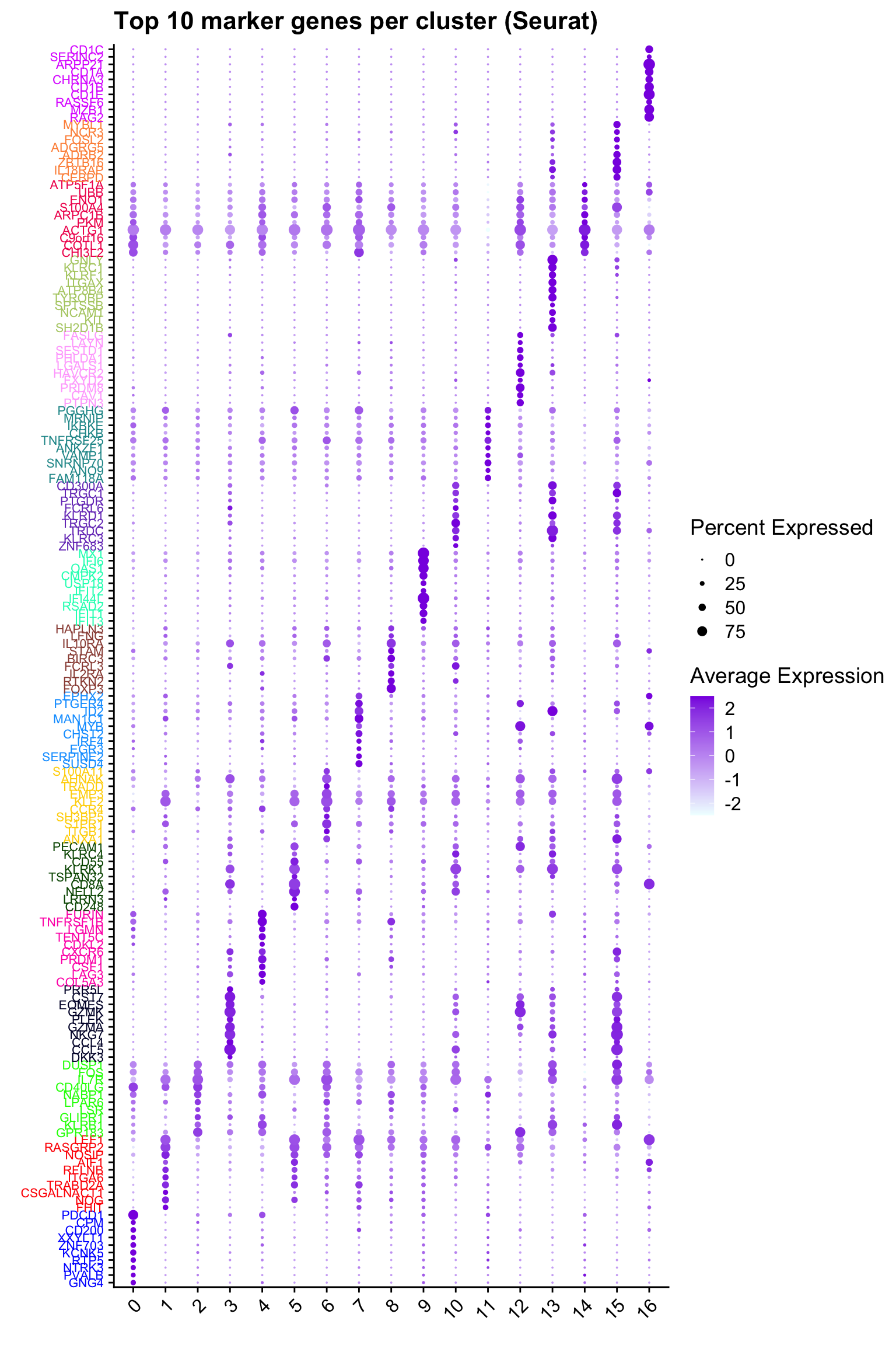
out_markers <- here("output",
            "CSV",
            paste(tissue,"_Marker_genes_Reclustered_Tcell_population.",opt_res, sep = ""))

dir.create(out_markers, recursive = TRUE, showWarnings = FALSE)

for (cl in unique(paed_sub.markers$cluster)) {
  cluster_data <- paed_sub.markers %>% dplyr::filter(cluster == cl)
  file_name <- here(out_markers, paste0("G000231_Neeland_",tissue, "_cluster_", cl, ".csv"))
  if (!file.exists(file_name)) {
  write.csv(cluster_data, file = file_name)
  }
}
Corresponding Azimuth labels (T cell subsets)
## Level 1
DimPlot(paed_sub, reduction = "umap.new", group.by = "predicted.celltype.l1", raster = FALSE, repel = TRUE, label = TRUE, label.size = 4.5) 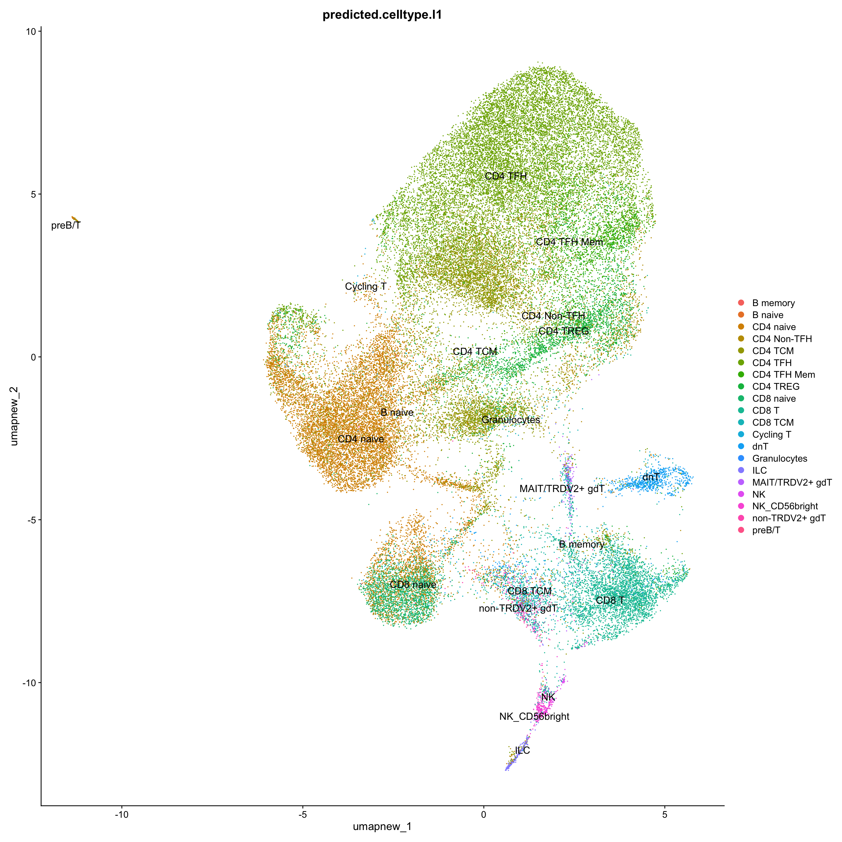
Excluding contaminating cells (B cell subtypes) for further clarity
sort(table(paed_sub$predicted.celltype.l1), decreasing = T)
        CD4 TFH       CD4 naive         CD4 TCM           CD8 T        CD4 TREG
          14687           10795            7709            3803            3352
    CD4 TFH Mem       CD8 naive     CD4 Non-TFH         CD8 TCM             dnT
           2700            2235            1574            1284            1056
 non-TRDV2+ gdT   NK_CD56bright             ILC MAIT/TRDV2+ gdT              NK
            347             260             258             156              83
      Cycling T         B naive        B memory    Granulocytes          preB/T
             22              13               4               1               1
exclude <- c("B memory", "B naive", "Granulocytes", "preB/T")
paed_sub_filtered <- paed_sub[, !paed_sub$predicted.celltype.l1 %in% exclude]
# Plots for Level 1
DimPlot(paed_sub_filtered, reduction = "umap.new", group.by = "predicted.celltype.l1", raster = FALSE, repel = TRUE, label = TRUE, label.size = 5) +
paletteer::scale_colour_paletteer_d("Polychrome::palette36")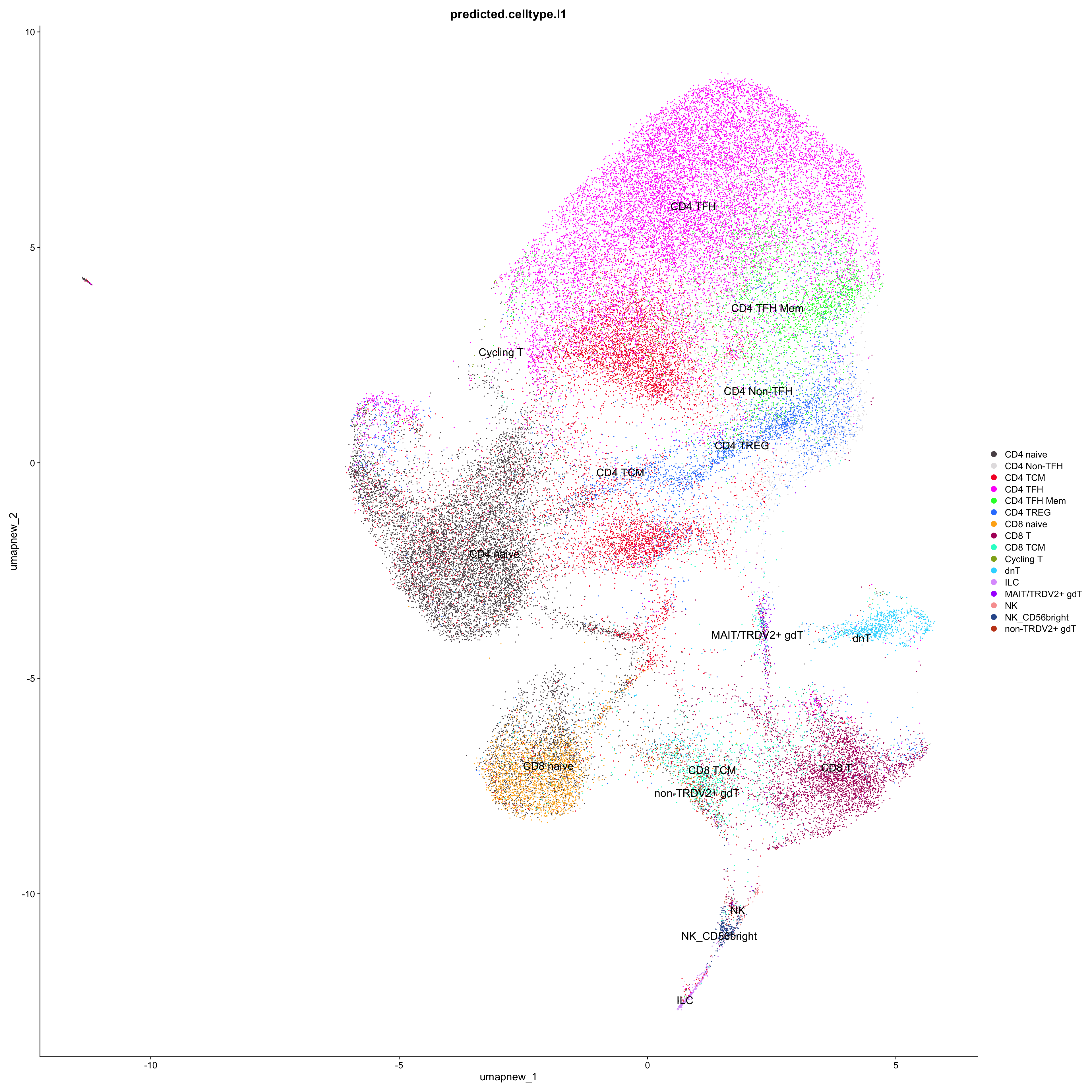
df_table_l1 <- as.data.frame(table(paed_sub_filtered$RNA_snn_res.0.4, paed_sub_filtered$predicted.celltype.l1))

ggplot(df_table_l1, aes(Var1, Freq, fill = Var2)) +
  geom_bar(stat = "identity") +
  labs(x = "RNA_snn_res.0.4", y = "Count", fill = "predicted.celltype.l1") +
  theme_minimal() +
  paletteer::scale_fill_paletteer_d("Polychrome::palette36") +
  ggtitle("Stacked Bar Plot of Tcell subsets (res=0.4) and predicted.celltype.l1")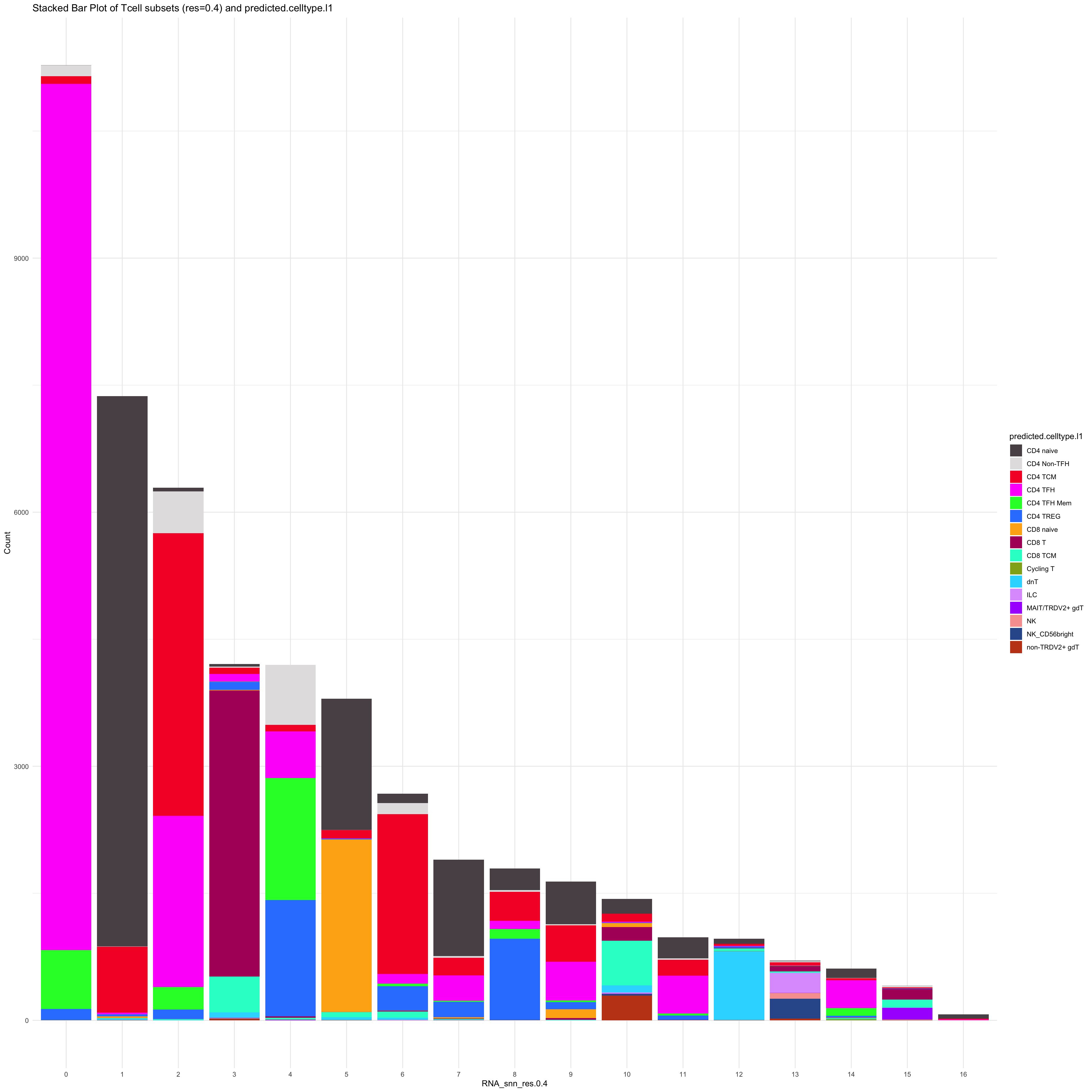
# Plots for Level 2
DimPlot(paed_sub_filtered, reduction = "umap.new", group.by = "predicted.celltype.l2", raster = FALSE, repel = TRUE, label = TRUE, label.size = 5)  +
    paletteer::scale_colour_paletteer_d("Polychrome::palette36")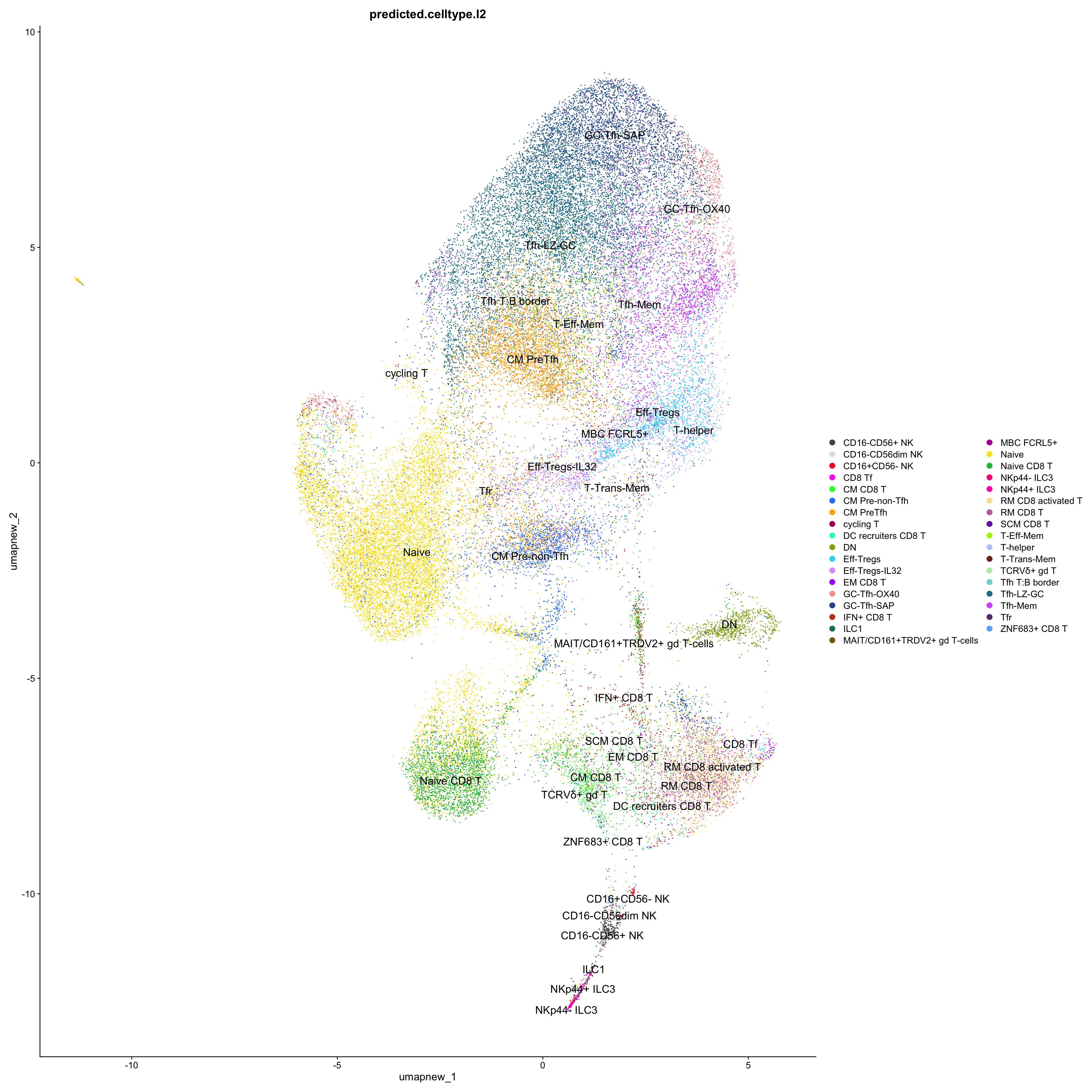
df_table_l2 <- as.data.frame(table(paed_sub_filtered$RNA_snn_res.0.4, paed_sub_filtered$predicted.celltype.l2))
ggplot(df_table_l2, aes(Var1, Freq, fill = Var2)) +
geom_bar(stat = "identity") +
labs(x = "RNA_snn_res.0.4", y = "Count", fill = "predicted.celltype.l2") +
theme_minimal() +
paletteer::scale_fill_paletteer_d("Polychrome::palette36") +
ggtitle("Stacked Bar Plot of Tcell subsets (res=0.4) and predicted.celltype.l2")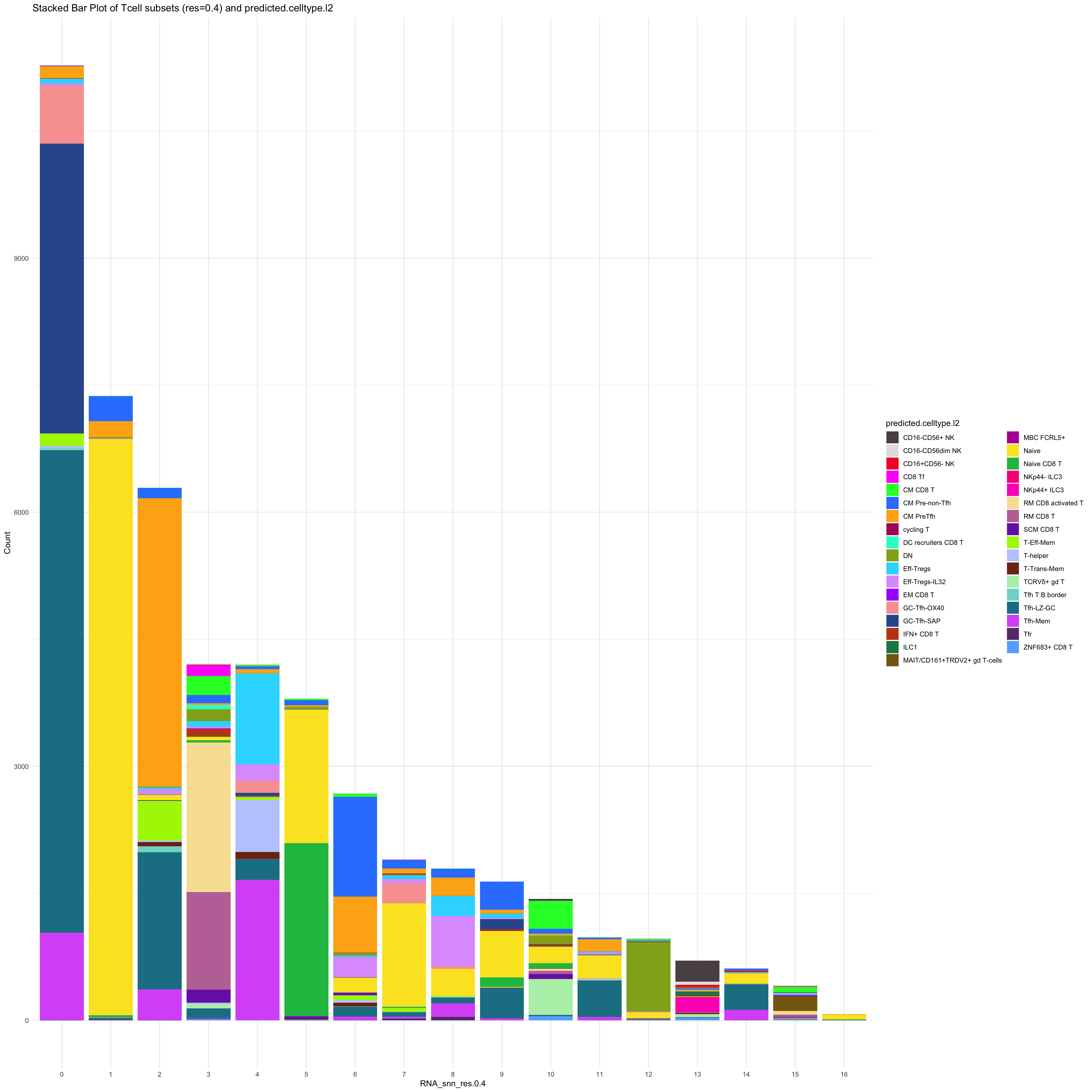 ## Update T subclustering labels
cell_labels <- readxl::read_excel(here("data/Cell_labels_Mel_v2/earlyAIR_Tonsil_and_Adenoid_T-NK_annotations_17.07.24.xlsx"), sheet = "Tonsil")
new_cluster_names <- cell_labels %>%
  dplyr::select(cluster, annotation) %>%
  deframe()

paed_sub <- RenameIdents(paed_sub, new_cluster_names)
paed_sub@meta.data$cell_labels_v2 <- Idents(paed_sub)

DimPlot(paed_sub, reduction = "umap.new", raster = FALSE, repel = TRUE, label = TRUE, label.size = 3.5) + ggtitle(paste0(tissue, ": UMAP with Updated subclustering"))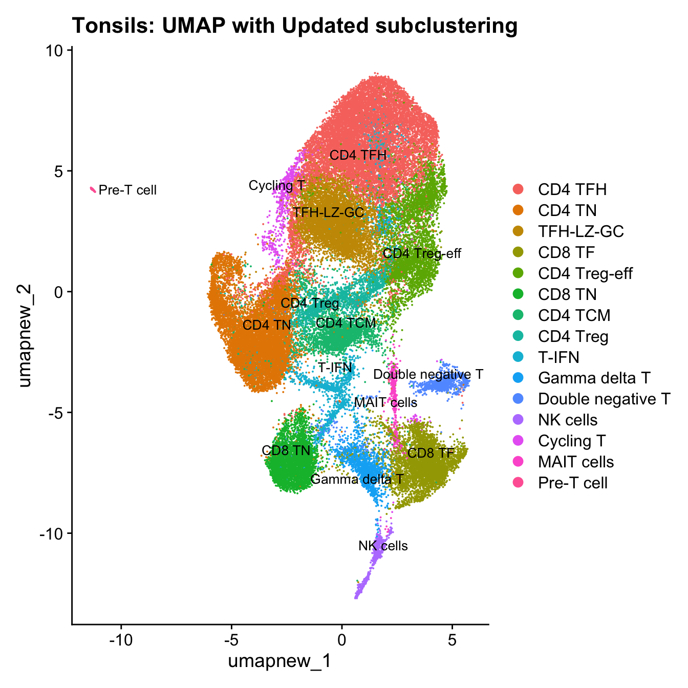
Save subclustered SEU object (Tcells)
out2 <- here("output",
            "RDS", "AllBatches_Subclustering_SEUs", tissue,
             paste0("G000231_Neeland_",tissue,".Tcell_population.subclusters.SEU.rds"))
#dir.create(out2)
if (!file.exists(out2)) {
  saveRDS(paed_sub, file = out2)
}
Reclustering GC cells
Reclustering clusters 2,5, 6, 11, 12
The marker genes for this reclustering can be found here-
sub_clusters <- c(2,5, 6, 11, 12)

idx <- which(merged_obj$cluster %in% sub_clusters)
paed_sub <- merged_obj[,idx]
paed_sub
An object of class Seurat
17566 features across 36470 samples within 1 assay
Active assay: RNA (17566 features, 2000 variable features)
3 layers present: data, counts, scale.data
4 dimensional reductions calculated: pca, umap.unintegrated, harmony, umap.harmony# Visualize the clustering results
DimPlot(paed_sub, reduction = "umap.harmony", group.by = "cluster", label = TRUE, label.size = 2.5, repel = TRUE, raster = FALSE )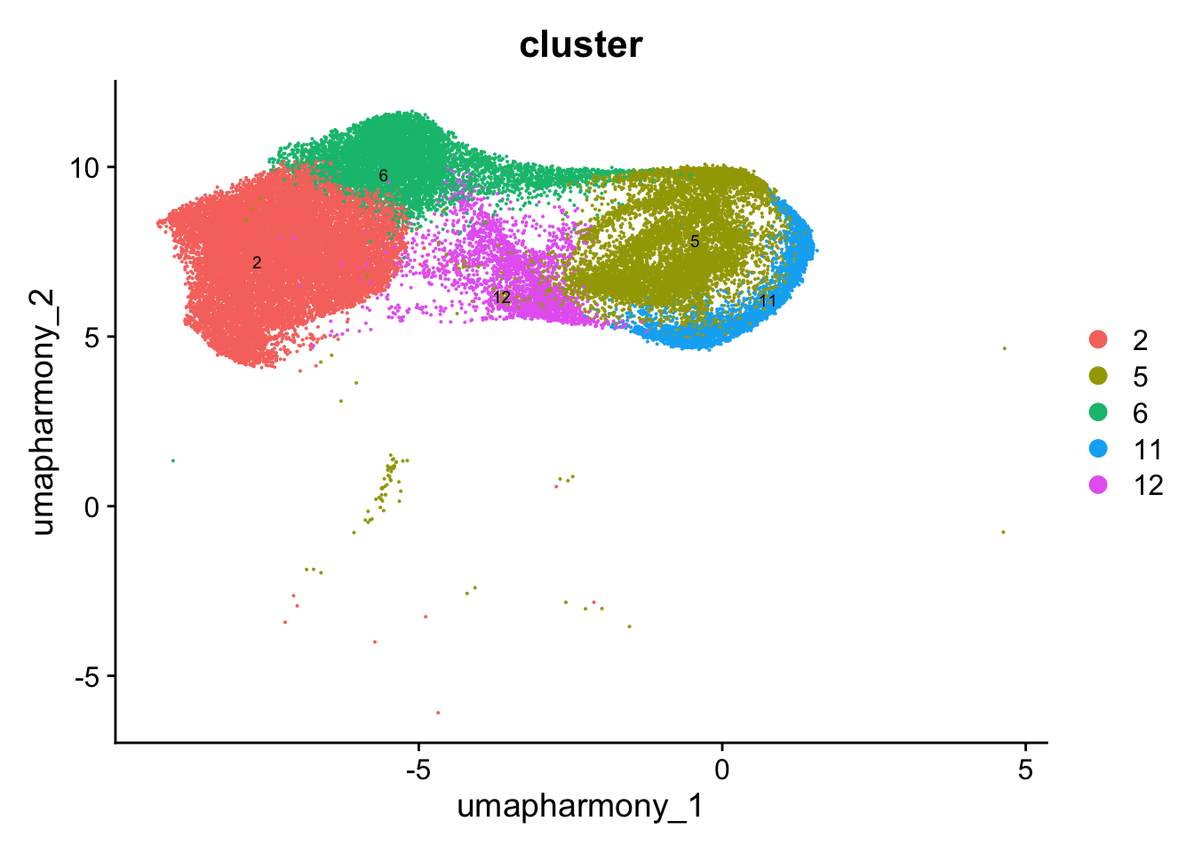
paed_sub <- paed_sub %>%
  NormalizeData() %>%
  FindVariableFeatures() %>%
  ScaleData() %>%
  RunPCA()

paed_sub <- RunUMAP(paed_sub, dims = 1:30, reduction = "pca", reduction.name = "umap.new")
meta_data_columns <- colnames(paed_sub@meta.data)
columns_to_remove <- grep("^RNA_snn_res", meta_data_columns, value = TRUE)
paed_sub@meta.data <- paed_sub@meta.data[, !(colnames(paed_sub@meta.data) %in% columns_to_remove)]resolutions <- seq(0.1, 1, by = 0.1)
paed_sub <- FindNeighbors(paed_sub, dims = 1:30, reduction = "pca")
paed_sub <- FindClusters(paed_sub, resolution = resolutions )Modularity Optimizer version 1.3.0 by Ludo Waltman and Nees Jan van Eck
Number of nodes: 36470
Number of edges: 1160680
Running Louvain algorithm...
Maximum modularity in 10 random starts: 0.9421
Number of communities: 4
Elapsed time: 5 seconds
Modularity Optimizer version 1.3.0 by Ludo Waltman and Nees Jan van Eck
Number of nodes: 36470
Number of edges: 1160680
Running Louvain algorithm...
Maximum modularity in 10 random starts: 0.9173
Number of communities: 8
Elapsed time: 5 seconds
Modularity Optimizer version 1.3.0 by Ludo Waltman and Nees Jan van Eck
Number of nodes: 36470
Number of edges: 1160680
Running Louvain algorithm...
Maximum modularity in 10 random starts: 0.9021
Number of communities: 11
Elapsed time: 5 seconds
Modularity Optimizer version 1.3.0 by Ludo Waltman and Nees Jan van Eck
Number of nodes: 36470
Number of edges: 1160680
Running Louvain algorithm...
Maximum modularity in 10 random starts: 0.8888
Number of communities: 13
Elapsed time: 6 seconds
Modularity Optimizer version 1.3.0 by Ludo Waltman and Nees Jan van Eck
Number of nodes: 36470
Number of edges: 1160680
Running Louvain algorithm...
Maximum modularity in 10 random starts: 0.8759
Number of communities: 15
Elapsed time: 4 seconds
Modularity Optimizer version 1.3.0 by Ludo Waltman and Nees Jan van Eck
Number of nodes: 36470
Number of edges: 1160680
Running Louvain algorithm...
Maximum modularity in 10 random starts: 0.8670
Number of communities: 15
Elapsed time: 5 seconds
Modularity Optimizer version 1.3.0 by Ludo Waltman and Nees Jan van Eck
Number of nodes: 36470
Number of edges: 1160680
Running Louvain algorithm...
Maximum modularity in 10 random starts: 0.8582
Number of communities: 17
Elapsed time: 5 seconds
Modularity Optimizer version 1.3.0 by Ludo Waltman and Nees Jan van Eck
Number of nodes: 36470
Number of edges: 1160680
Running Louvain algorithm...
Maximum modularity in 10 random starts: 0.8498
Number of communities: 18
Elapsed time: 5 seconds
Modularity Optimizer version 1.3.0 by Ludo Waltman and Nees Jan van Eck
Number of nodes: 36470
Number of edges: 1160680
Running Louvain algorithm...
Maximum modularity in 10 random starts: 0.8425
Number of communities: 19
Elapsed time: 4 seconds
Modularity Optimizer version 1.3.0 by Ludo Waltman and Nees Jan van Eck
Number of nodes: 36470
Number of edges: 1160680
Running Louvain algorithm...
Maximum modularity in 10 random starts: 0.8344
Number of communities: 20
Elapsed time: 5 secondsclustree(paed_sub, prefix = "RNA_snn_res.")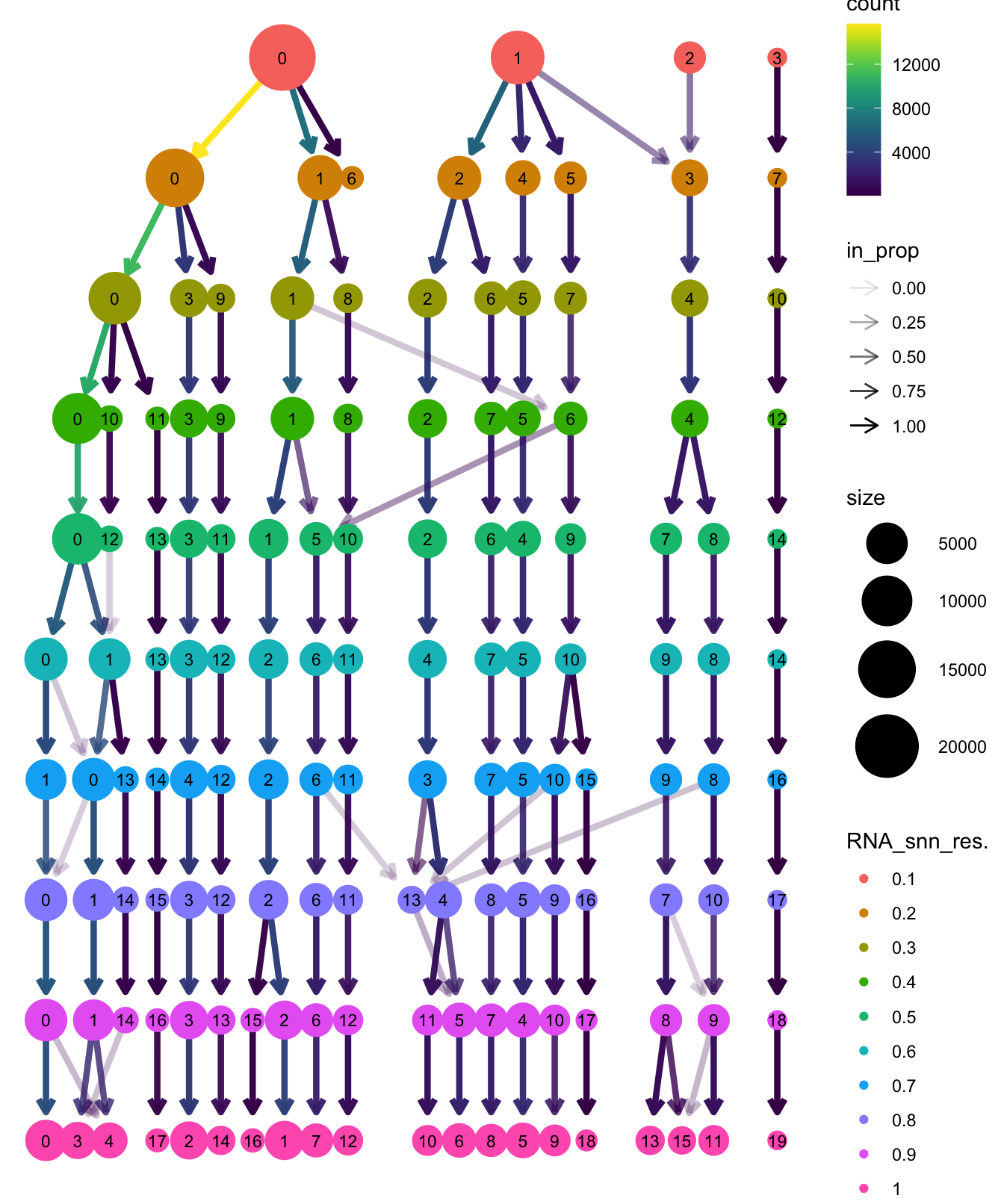
# Visualize the clustering results
DimPlot(paed_sub, group.by = "RNA_snn_res.0.6", reduction = "umap.new", label = TRUE, label.size = 2.5, repel = TRUE, raster = FALSE )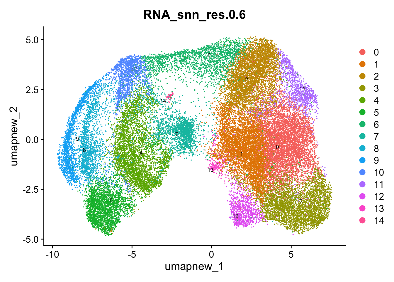
opt_res <- "RNA_snn_res.0.6"
n <- nlevels(paed_sub$RNA_snn_res.0.6)
paed_sub$RNA_snn_res.0.6 <- factor(paed_sub$RNA_snn_res.0.6, levels = seq(0,n-1))
paed_sub$seurat_clusters <- NULL
paed_sub$cluster <- paed_sub$RNA_snn_res.0.6
Idents(paed_sub) <- paed_sub$cluster
paed_sub.markers <- FindAllMarkers(paed_sub, only.pos = TRUE, min.pct = 0.25, logfc.threshold = 0.25)Calculating cluster 0Calculating cluster 1Calculating cluster 2Calculating cluster 3Calculating cluster 4Calculating cluster 5Calculating cluster 6Calculating cluster 7Calculating cluster 8Calculating cluster 9Calculating cluster 10Calculating cluster 11Calculating cluster 12Calculating cluster 13Calculating cluster 14paed_sub.markers %>%
group_by(cluster) %>% unique() %>%
top_n(n = 5, wt = avg_log2FC) -> top5
paed_sub.markers %>%
group_by(cluster) %>%
slice_head(n=1) %>%
pull(gene) -> best.wilcox.gene.per.cluster
best.wilcox.gene.per.cluster [1] "HVCN1" "LMO2" "SLC30A4" "BCL2A1" "TYMS" "MCM4"
[7] "STMN1" "TRBC2" "HIST1H2BH" "HIST1H2BB" "CDC20" "PTPRJ"
[13] "PRDM1" "XAF1" "GIMAP4" Feature plot shows the expression of top marker genes per cluster.
FeaturePlot(paed_sub,features=best.wilcox.gene.per.cluster, reduction = 'umap.new', raster = FALSE, ncol = 2, label = TRUE)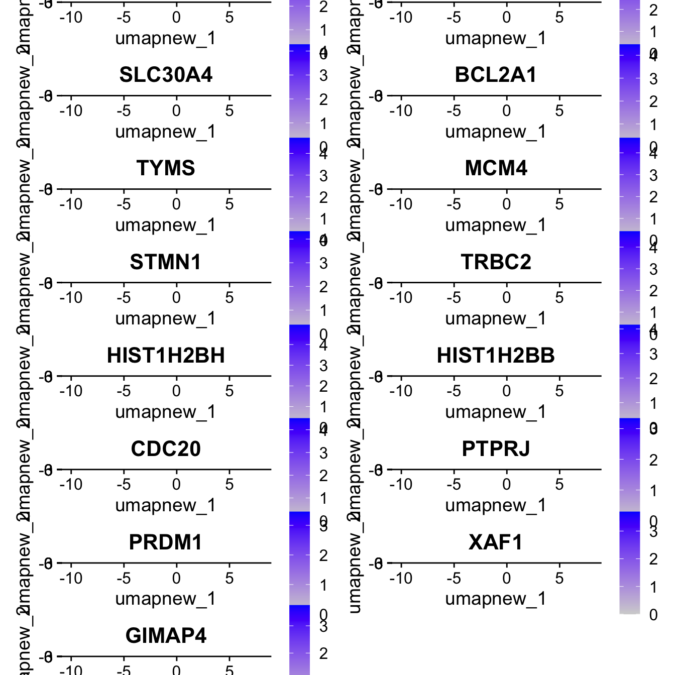
Top 10 marker genes from Seurat
## Seurat top markers
top10 <- paed_sub.markers %>%
    group_by(cluster) %>%
    top_n(n = 10, wt = avg_log2FC) %>%
    ungroup() %>%
    distinct(gene, .keep_all = TRUE) %>%
    arrange(cluster, desc(avg_log2FC))

cluster_colors <- paletteer::paletteer_d("pals::glasbey")[factor(top10$cluster)]

DotPlot(paed_sub,
        features = unique(top10$gene),
        group.by = opt_res,
        cols = c("azure1", "blueviolet"),
        dot.scale = 3, assay = "RNA") +
    RotatedAxis() +
    FontSize(y.text = 8, x.text = 12) +
    labs(y = element_blank(), x = element_blank()) +
    coord_flip() +
    theme(axis.text.y = element_text(color = cluster_colors)) +
    ggtitle("Top 10 marker genes per cluster (Seurat)")
Warning: Vectorized input to `element_text()` is not officially supported.
ℹ Results may be unexpected or may change in future versions of ggplot2.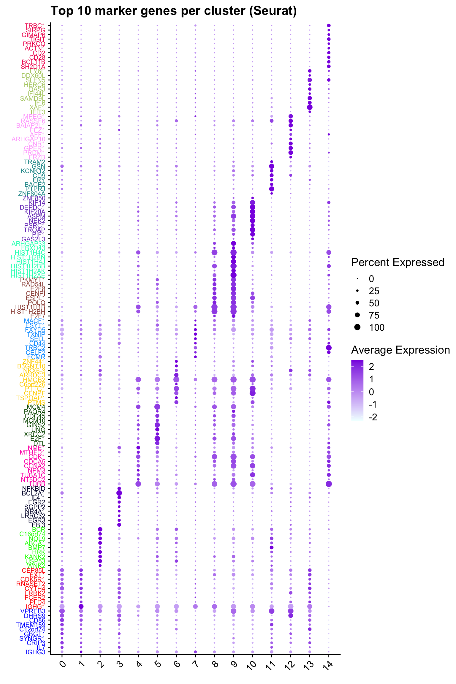
out_markers <- here("output",
            "CSV",
            paste(tissue,"_Marker_genes_Reclustered_GC_population.",opt_res, sep = ""))

dir.create(out_markers, recursive = TRUE, showWarnings = FALSE)

for (cl in unique(paed_sub.markers$cluster)) {
  cluster_data <- paed_sub.markers %>% dplyr::filter(cluster == cl)
  file_name <- here(out_markers, paste0("G000231_Neeland_",tissue, "_cluster_", cl, ".csv"))
  if (!file.exists(file_name)) {
  write.csv(cluster_data, file = file_name)
  }
}
Corresponding Azimuth labels (GC cell subsets)
## Level 1
DimPlot(paed_sub, reduction = "umap.new", group.by = "predicted.celltype.l1", raster = FALSE, repel = TRUE, label = TRUE, label.size = 4.5) 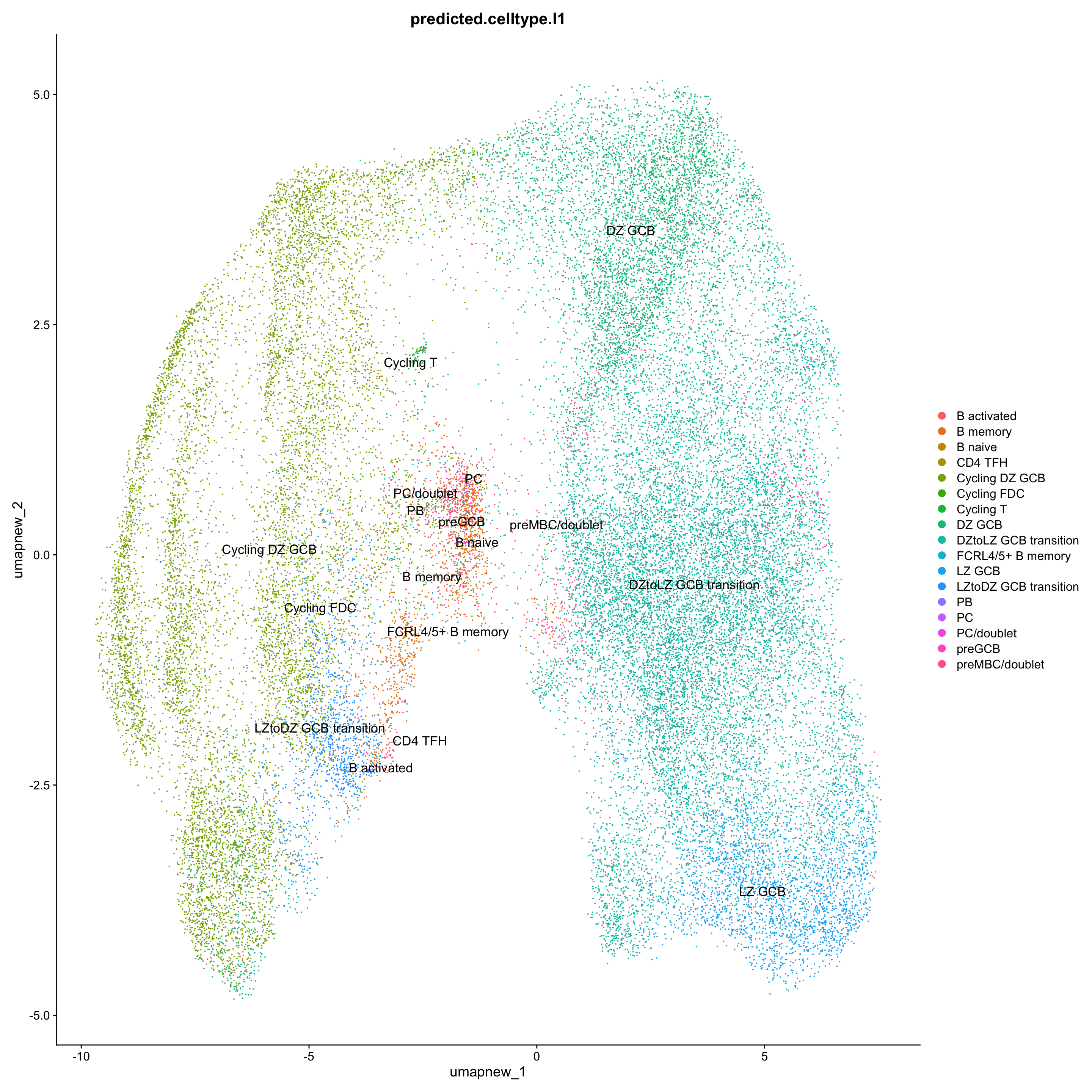
df_table <- as.data.frame(table(paed_sub$RNA_snn_res.0.6, paed_sub$predicted.celltype.l1))
ggplot(df_table, aes(Var1, Freq, fill = Var2)) +
  geom_bar(stat = "identity") +
  labs(x = "RNA_snn_res.0.6", y = "Count", fill = "predicted.celltype.l1") +
  theme_minimal() +
  ggtitle("Stacked Bar Plot of Tcell subsets (res=0.6) and predicted.celltype.l1")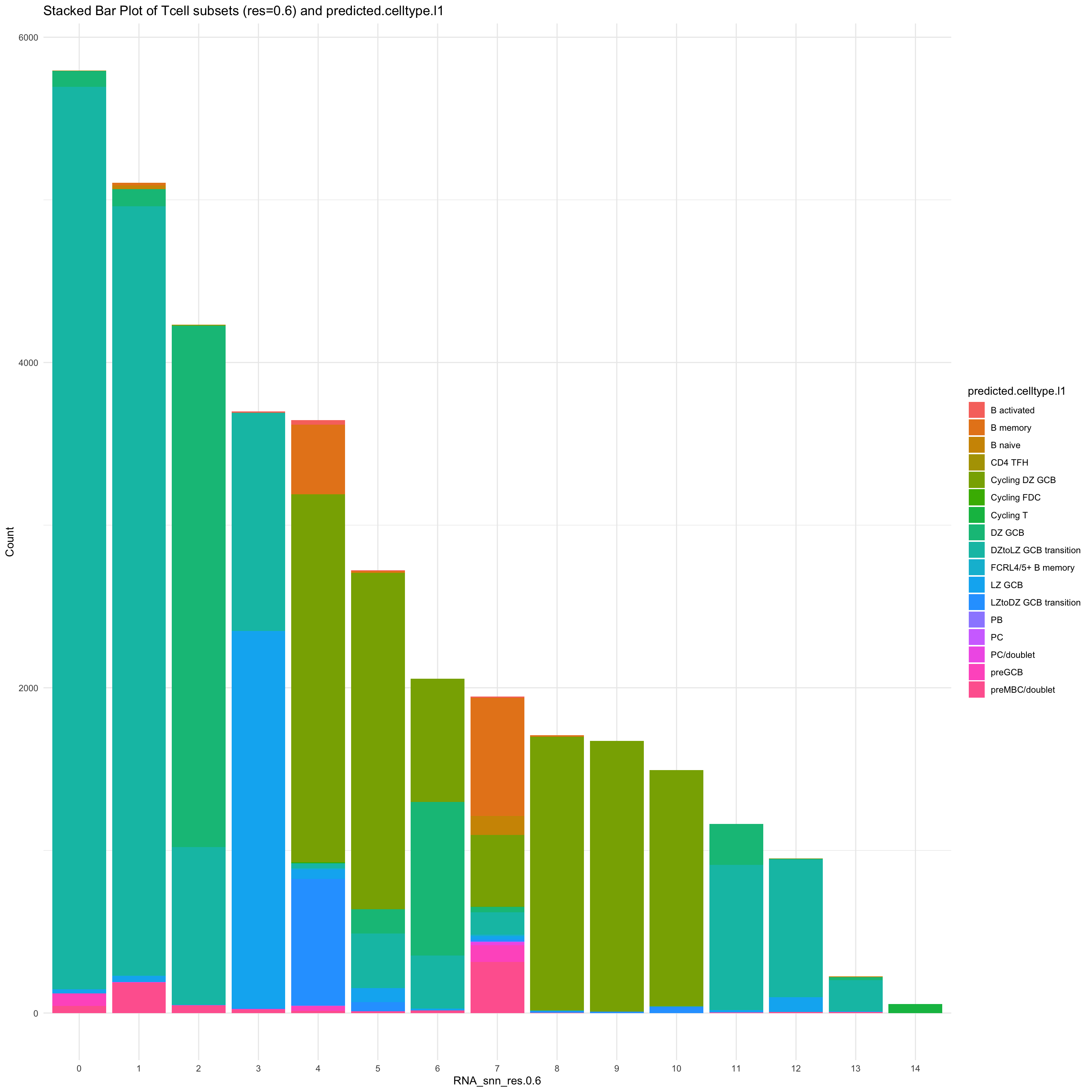
Update GC subclustering labels
cell_labels <- readxl::read_excel(here("data/Cell_labels_Mel_v2/earlyAIR_Tonsil_and_Adenoid_GC-B cell annotations_09.08.24.xlsx"), sheet = "Tonsil")
new_cluster_names <- cell_labels %>%
  dplyr::select(cluster, annotation) %>%
  deframe()

paed_sub <- RenameIdents(paed_sub, new_cluster_names)
paed_sub@meta.data$cell_labels_v2 <- Idents(paed_sub)

DimPlot(paed_sub, reduction = "umap.new", raster = FALSE, repel = TRUE, label = TRUE, label.size = 3.5) + ggtitle(paste0(tissue, ": UMAP with Updated subclustering"))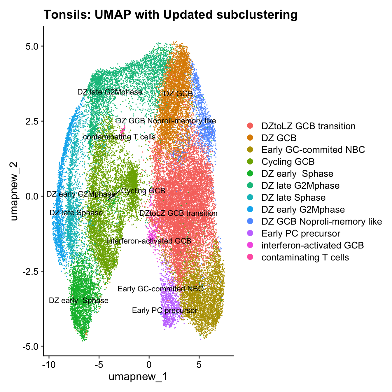
palette1 <- paletteer::paletteer_d("ggthemes::Classic_20")
palette2 <- paletteer::paletteer_d("Polychrome::light")
combined_palette <- unique(c(palette1, palette2))

labels <- c( "cell_labels", "cell_labels_v2", "RNA_snn_res.0.6", "predicted.celltype.l1", "Broad_cell_label_3")

p <- vector("list",length(labels))
for(label in labels){
  paed_sub@meta.data %>%
    ggplot(aes(x = !!sym(label),
               fill = !!sym(label))) +
    geom_bar() +
    geom_text(aes(label = ..count..), stat = "count",
              vjust = -0.5, colour = "black", size = 2) +
    scale_y_log10() +
    theme(axis.text.x = element_blank(),
          axis.title.x = element_blank(),
          axis.ticks.x = element_blank()) +
    NoLegend() +
    labs(y = "No. Cells (log scale)") -> p1

  paed_sub@meta.data %>%
    dplyr::select(!!sym(label), Sample) %>%
    group_by(!!sym(label), Sample) %>%
    summarise(num = n()) %>%
    mutate(prop = num / sum(num)) %>%
  ggplot(aes(x = !!sym(label), y = prop * 100,
             fill = Sample)) +
    geom_bar(stat = "identity") +
    theme(axis.text.x = element_text(angle = 90,
                                     vjust = 0.5,
                                     hjust = 1,
                                     size = 8)) +
    labs(y = "% Cells", fill = "Sample") +
  scale_fill_manual(values = combined_palette) -> p2

  (p1 / p2) & theme(legend.text = element_text(size = 8),
                  legend.key.size = unit(3, "mm")) -> p[[label]]
}
`summarise()` has grouped output by 'cell_labels'. You can override using the
`.groups` argument.
`summarise()` has grouped output by 'cell_labels_v2'. You can override using
the `.groups` argument.
`summarise()` has grouped output by 'RNA_snn_res.0.6'. You can override using
the `.groups` argument.
`summarise()` has grouped output by 'predicted.celltype.l1'. You can override
using the `.groups` argument.
`summarise()` has grouped output by 'Broad_cell_label_3'. You can override
using the `.groups` argument.p[[1]]
NULL
[[2]]
NULL
[[3]]
NULL
[[4]]
NULL
[[5]]
NULL
$cell_labelsWarning: The dot-dot notation (`..count..`) was deprecated in ggplot2 3.4.0.
ℹ Please use `after_stat(count)` instead.
This warning is displayed once every 8 hours.
Call `lifecycle::last_lifecycle_warnings()` to see where this warning was
generated.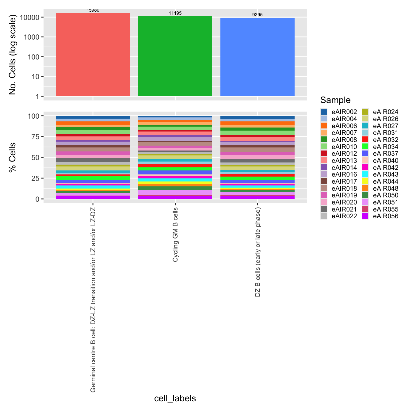
$cell_labels_v2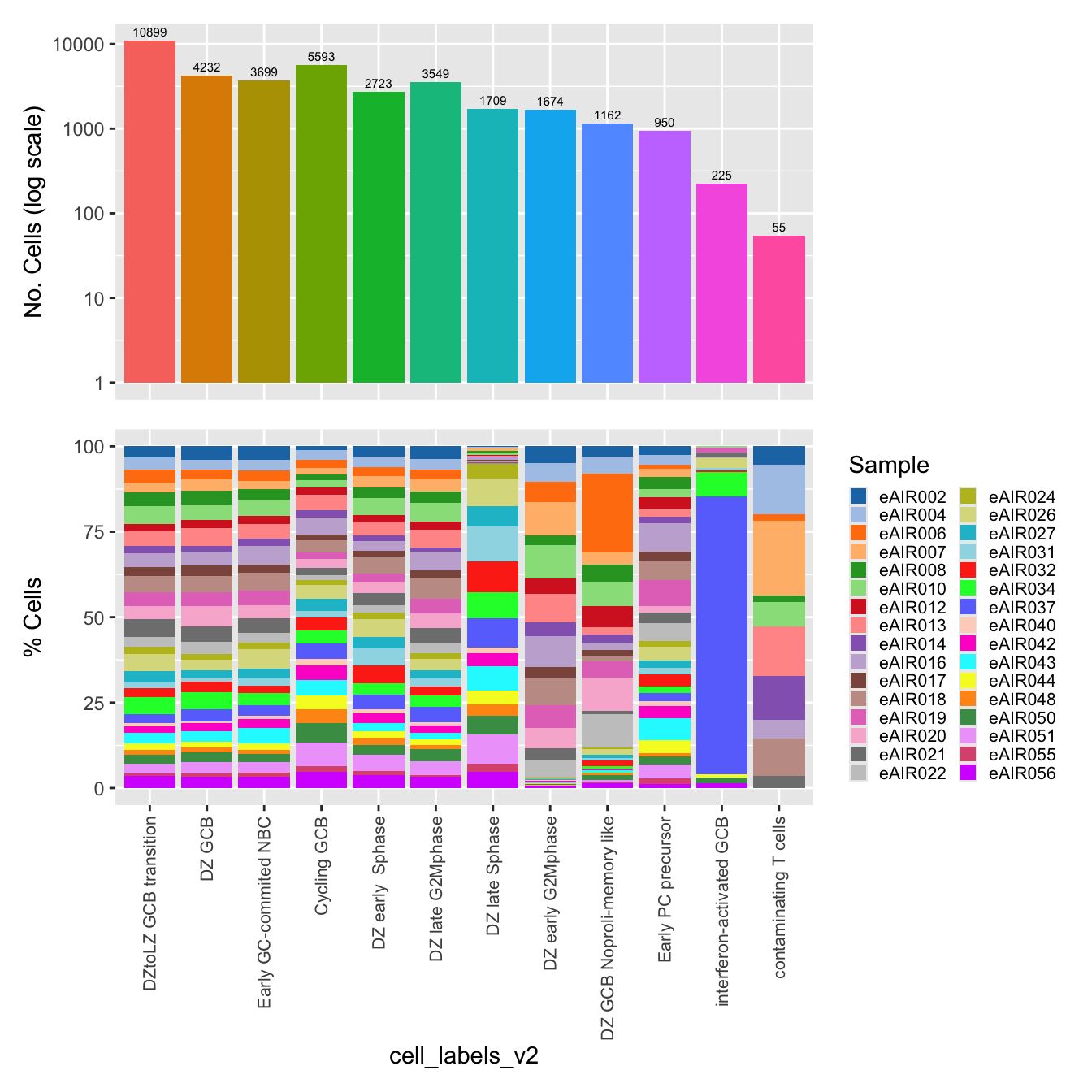
$RNA_snn_res.0.6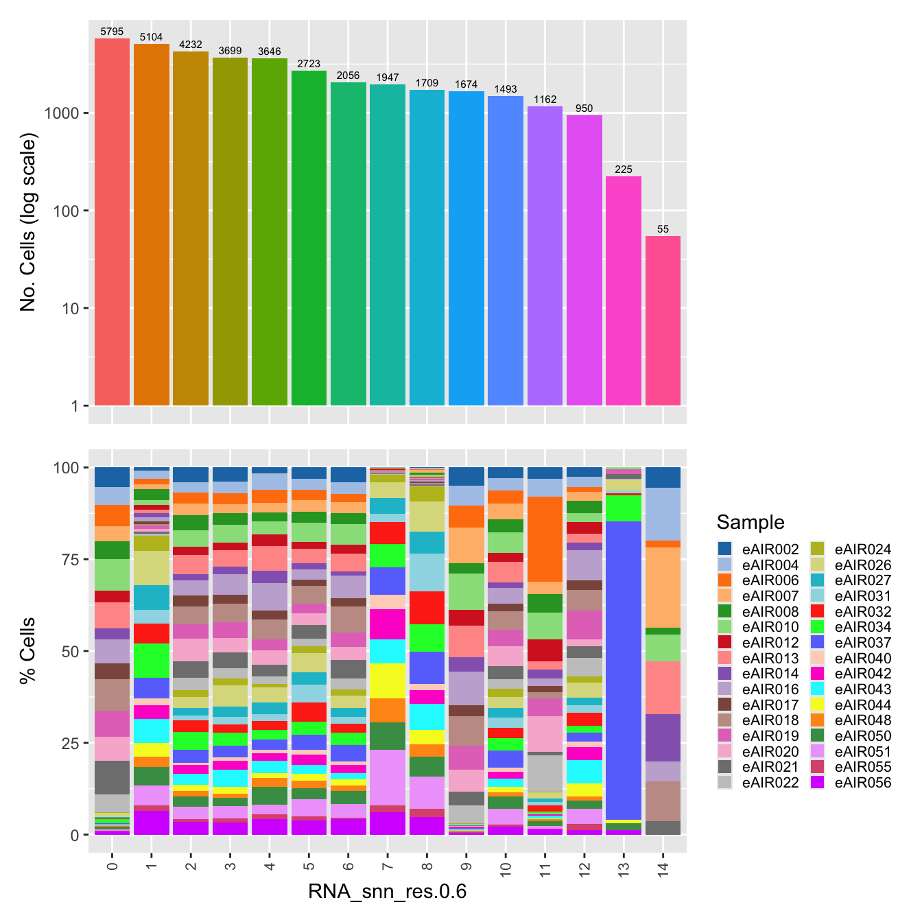
$predicted.celltype.l1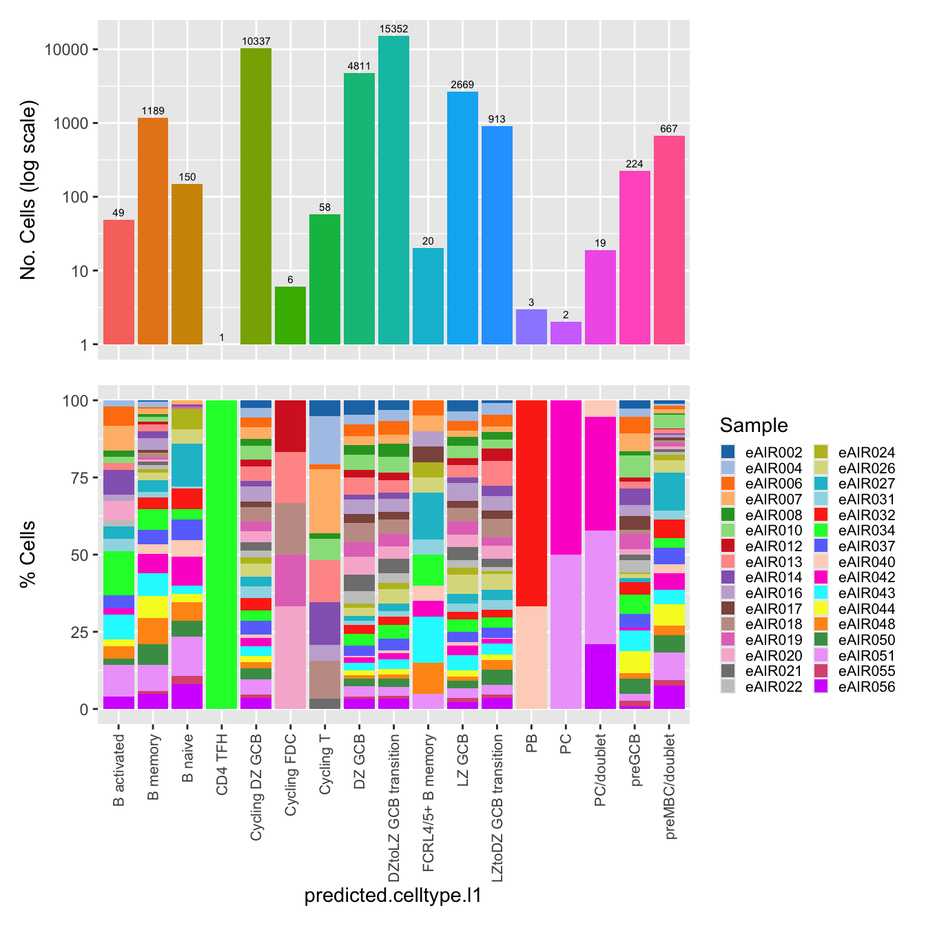
$Broad_cell_label_3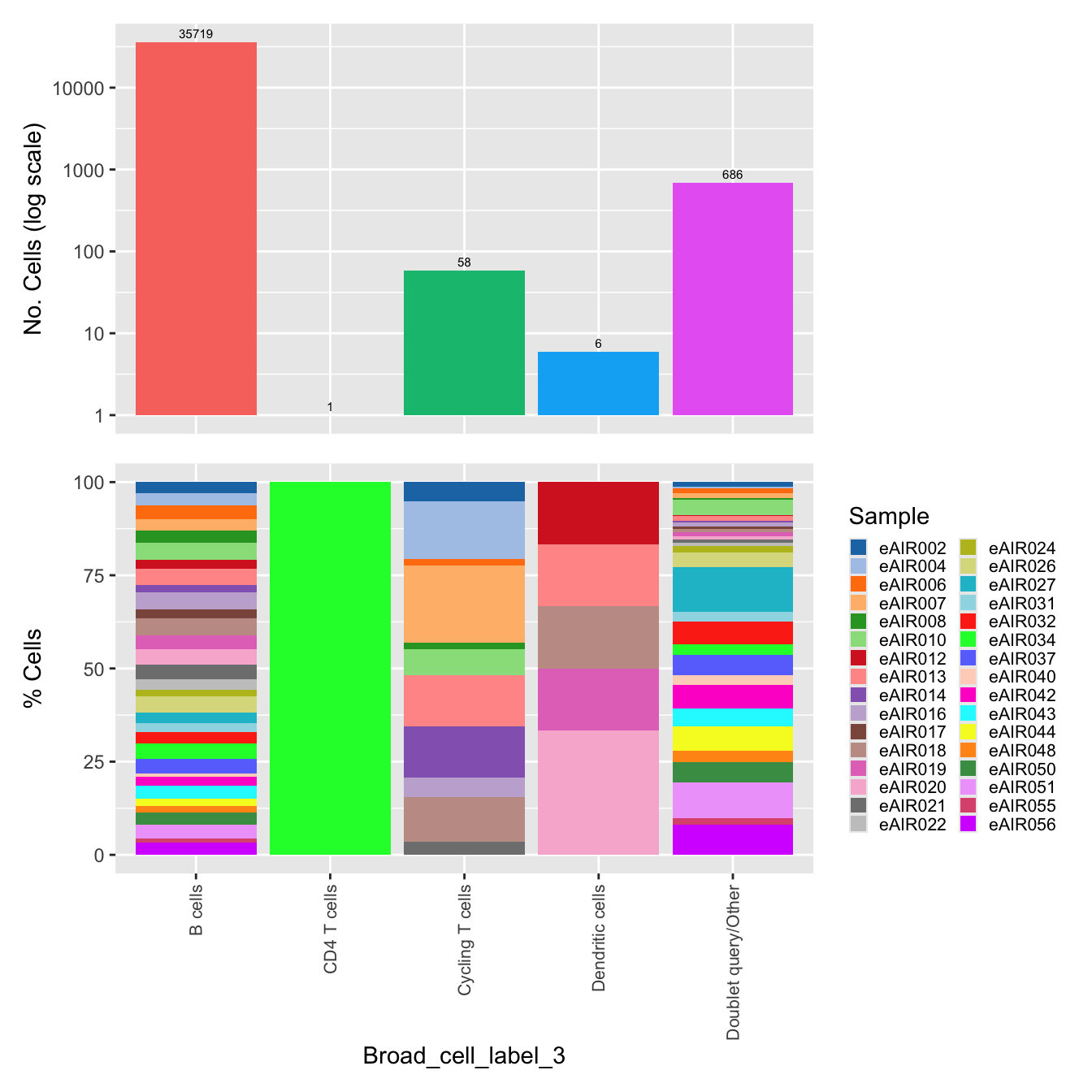
Save subclustered SEU object
out2 <- here("output",
            "RDS", "AllBatches_Subclustering_SEUs", tissue,
             paste0("G000231_Neeland_",tissue,".GC_population.subclusters.SEU.rds"))
#dir.create(out2)
if (!file.exists(out2)) {
  saveRDS(paed_sub, file = out2)
}
Confirm cluster 13 (activated DC3)
From Mel’s notes: Confirming CCR7 and LAMP3 expression in cluster 13 currently labelled as “activated DC3 (aDC3)?”
idx <- which(merged_obj$cluster %in% 13)
paed_sub <- merged_obj[,idx]
paed_sub
An object of class Seurat
17566 features across 2349 samples within 1 assay
Active assay: RNA (17566 features, 2000 variable features)
3 layers present: data, counts, scale.data
4 dimensional reductions calculated: pca, umap.unintegrated, harmony, umap.harmonyFeaturePlot(paed_sub,features=c("CCR7","LAMP3"), reduction = 'umap.harmony', ncol = 1, label = FALSE)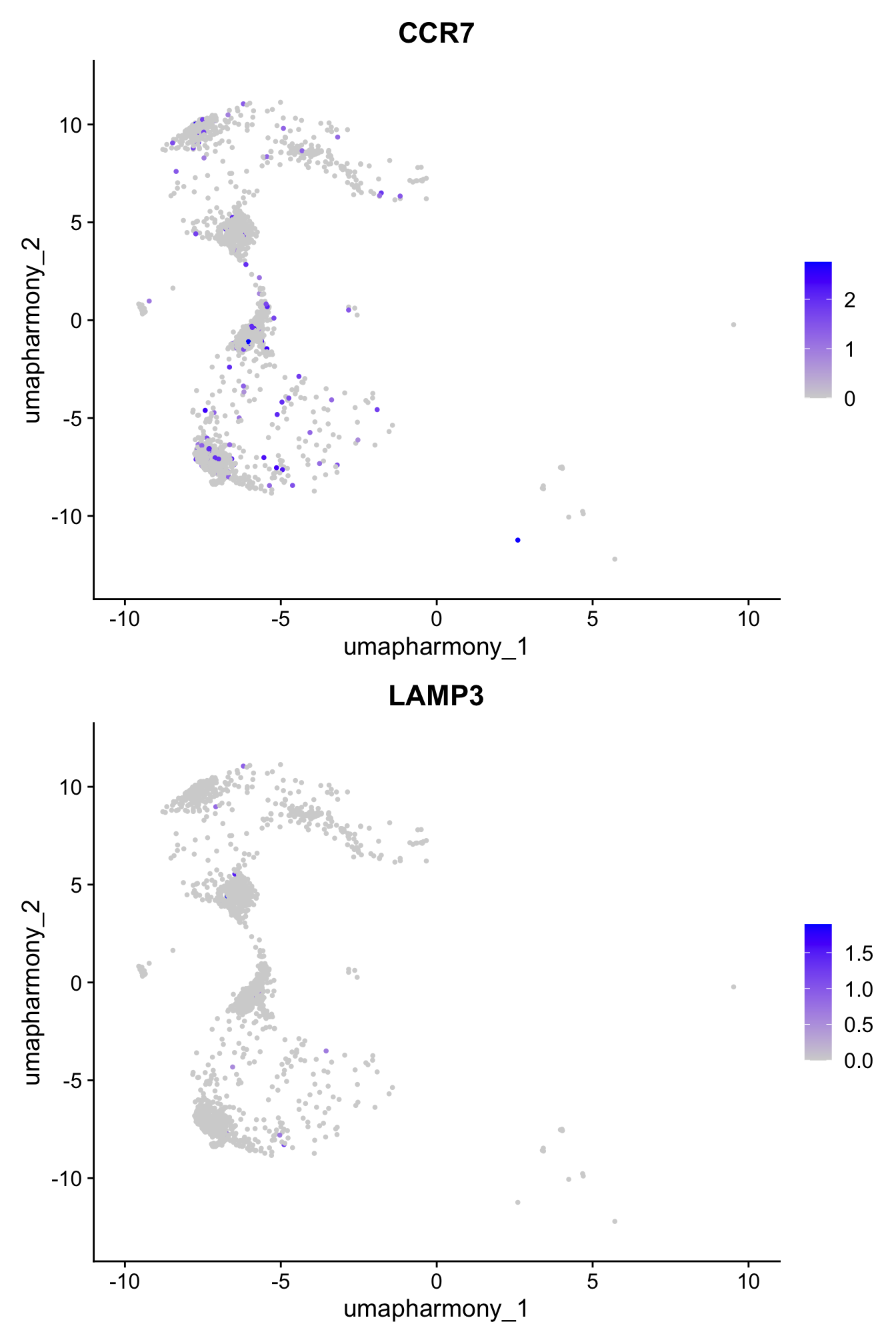
Other Clusters (excluding subclusters)
sub_clusters <- c(1, 4, 7, 8, 10, 17, 19, 20, 22, 2,5, 6, 11, 12)

idx <- which(merged_obj$cluster %in% sub_clusters)
paed_sub <- merged_obj[,-idx]
paed_sub
An object of class Seurat
17566 features across 54895 samples within 1 assay
Active assay: RNA (17566 features, 2000 variable features)
3 layers present: data, counts, scale.data
4 dimensional reductions calculated: pca, umap.unintegrated, harmony, umap.harmonylevels(paed_sub$cell_labels)[levels(paed_sub$cell_labels) == "activated DC3 (aDC3)?"] <- "activated DC3 (aDC3)"
levels(Idents(paed_sub))[levels(Idents(paed_sub)) == "activated DC3 (aDC3)?"] <- "activated DC3 (aDC3)"
paed_sub$cell_labels_v2 <- Idents(paed_sub)# Visualize the clustering results
DimPlot(paed_sub, reduction = "umap.harmony", group.by = "cluster", label = TRUE, label.size = 2.5, repel = TRUE, raster = FALSE )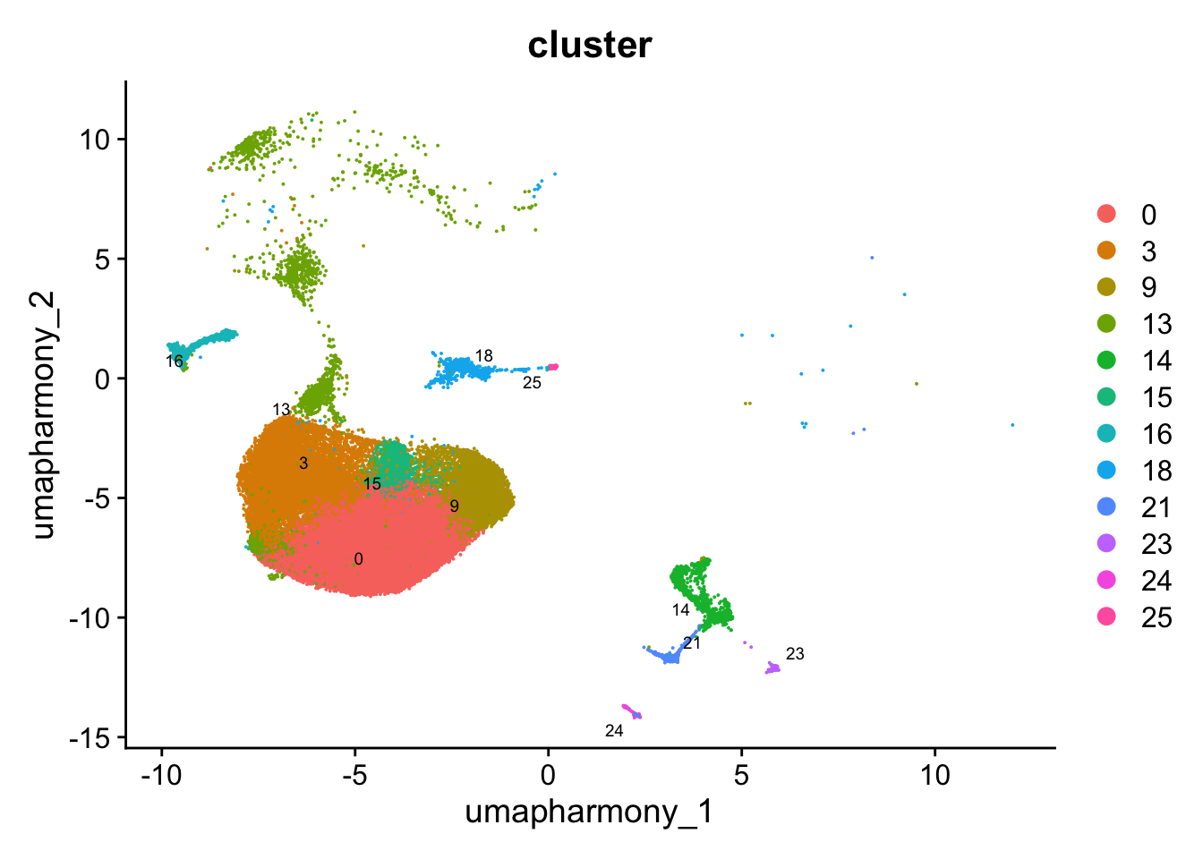
DimPlot(paed_sub, reduction = "umap.harmony", label = TRUE, label.size = 2.5, repel = TRUE, raster = FALSE )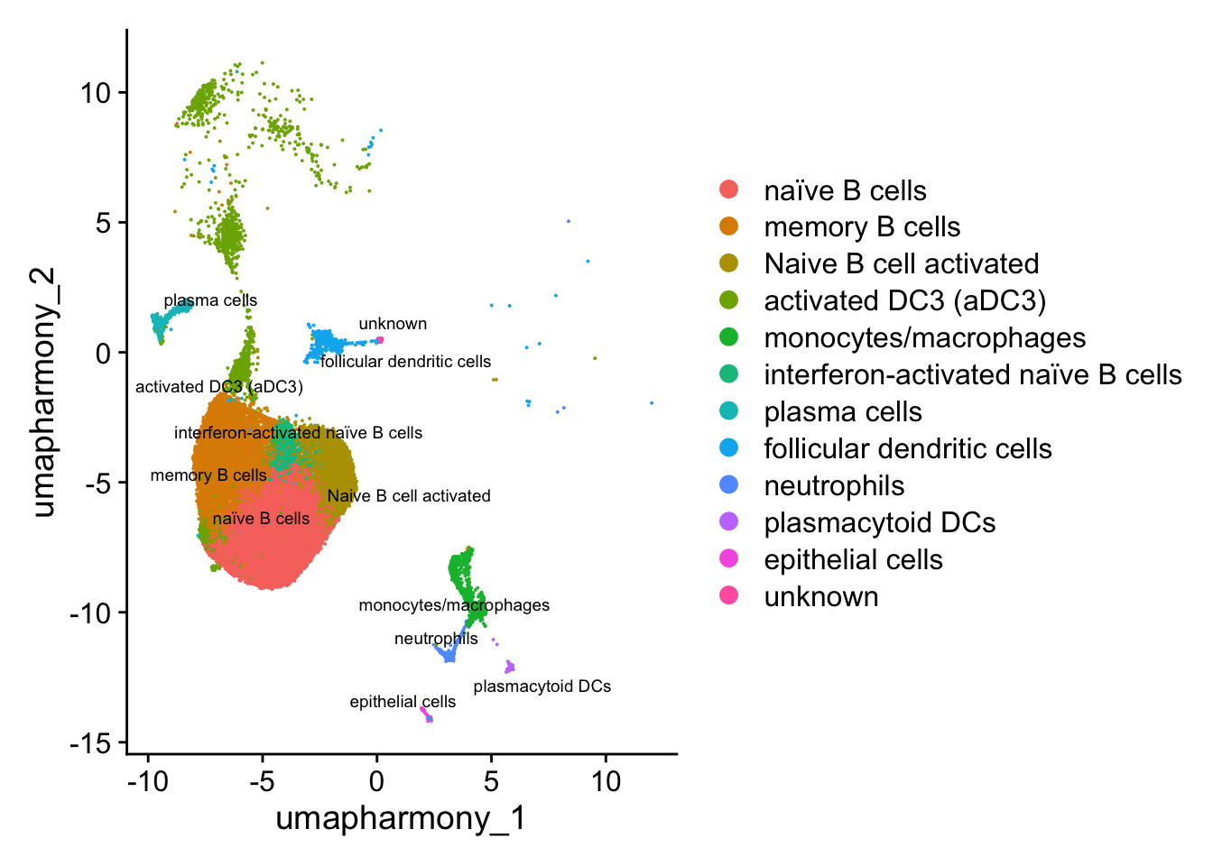
Save subclustered SEU object ( All other cells)
out2 <- here("output",
            "RDS", "AllBatches_Subclustering_SEUs", tissue,
             paste0("G000231_Neeland_",tissue,".all_other.subclusters.SEU.rds"))
#dir.create(out2)
if (!file.exists(out2)) {
  saveRDS(paed_sub, file = out2)
}
Merge seurat objects of subclusters
files <- list.files(here("output",
            "RDS", "AllBatches_Subclustering_SEUs", tissue),
                    full.names = TRUE)

seuLst <- lapply(files, function(f) readRDS(f))

seu <- merge(seuLst[[1]],
             y = c(seuLst[[2]],
                   seuLst[[3]]))
seu
An object of class Seurat
17566 features across 141705 samples within 1 assay
Active assay: RNA (17566 features, 2000 variable features)
9 layers present: data.1, data.2, data.3, counts.1, scale.data.1, counts.2, scale.data.2, counts.3, scale.data.3Excluding contaminating labels
idx <- which(grepl("^contaminating", Idents(seu)))
seu <- seu[, -idx]
merged <- seu %>%
NormalizeData() %>%
FindVariableFeatures() %>%
ScaleData() %>%
RunPCA()Normalizing layer: counts.1Normalizing layer: counts.2Normalizing layer: counts.3Finding variable features for layer counts.1Finding variable features for layer counts.2Finding variable features for layer counts.3Centering and scaling data matrixPC_ 1
Positive: TRBC2, CD44, CD3D, CD3E, FYB1, TCF7, GIMAP7, GIMAP4, IL32, SPOCK2
LCP2, SELL, TRBC1, CD4, CD7, SRGN, CD28, IL7R, CD96, ITM2A
MAF, CCR7, CD69, ARL4C, KLF2, IL2RB, GBP2, PLAC8, DDIT4, ICOS
Negative: MKI67, KIFC1, NUSAP1, MYBL2, AURKB, TYMS, CDK1, TOP2A, STMN1, TK1
TPX2, NCAPG, HMGB2, BIRC5, ZWINT, CCNB2, KIF11, RRM2, HIST1H1B, FOXM1
RGS13, HJURP, MEF2B, ASF1B, CCNA2, UHRF1, CDT1, CDCA8, KIF2C, BUB1
PC_ 2
Positive: CD3D, CD3E, IL32, FYB1, TCF7, GIMAP7, GIMAP4, LCP2, SRGN, CD28
MAF, CD4, TRBC1, ITM2A, CD7, IL2RB, TRBC2, SPN, ICOS, TIGIT
SPOCK2, SH2D1A, IL7R, CD40LG, ST8SIA1, TOX2, PDCD1, HNRNPLL, TBC1D4, ZNRF1
Negative: MS4A1, CD22, CIITA, BANK1, IGHM, FCRL1, WDFY4, CD19, IGHD, FCRL2
CD83, BTK, IFI30, TCL1A, PHACTR1, FCER2, SYNGR2, FCRL5, MPEG1, CR1
CTSH, ADAM19, CCR6, CD24, SEMA7A, FCRL3, PARP15, VPREB3, FAM30A, SNX22
PC_ 3
Positive: MEF2B, BCL6, LHFPL2, RGS13, LMO2, SYNE2, PDCD1, CD38, TOX2, EML6
CAMK1, POU2AF1, ELL3, PTPRS, SIAH2, MAF, MME, CD82, DHRS9, IL21
GNG4, SCARB1, BCL2L11, ST14, SMCO4, PFKFB3, KIAA1324, ZC3H12D, CPM, CD27
Negative: KLF2, SELL, PLAC8, VIM, S1PR1, PARP15, CXCR4, KIF23, PLK1, CDC20
KIF20A, HJURP, DLGAP5, CCR6, HMMR, CENPA, CDCA8, KLRK1, TOP2A, CCR7
NEK2, KIF14, AURKB, ASPM, GTSE1, KIFC1, CCNB2, CD44, IGHD, DEPDC1
PC_ 4
Positive: CXCR4, TOX2, CXCR5, PDCD1, IKZF3, LTB, CHI3L2, IGHM, ST8SIA1, IGHD
CD40LG, TRBC2, ICOS, TRIB2, ITM2A, MAF, SARDH, RTP5, GNG4, BANK1
SESN3, IL21, TIGIT, FAM43A, KIAA1324, ZNF703, GLCCI1, SPOCK2, KCNK5, TBC1D4
Negative: LYZ, PTGDS, TMEM176B, SERPINF1, MMP9, ITGAX, ENPP2, CD68, APOE, CSF2RA
FCER1G, RASSF4, MS4A6A, TNFAIP2, SPARC, CST3, IL18, PLA2G2D, TYROBP, GLUL
MAFB, SLCO2B1, LMNA, GPNMB, CSF1R, GSN, COL6A1, MMP14, CD14, NPL
PC_ 5
Positive: PTGDS, LYZ, TOX2, KIF20A, PLK1, CENPA, KIF14, HMMR, CDC20, CENPE
NEK2, ASPM, TROAP, PDCD1, TMEM176B, CENPF, MMP9, ENPP2, PSRC1, PIF1
AURKA, APOE, CCNB2, PLXND1, SERPINF1, MAF, DLGAP5, CLEC7A, DEPDC1, MAFB
Negative: CCL5, KLRK1, NKG7, CD8A, SAMD3, GZMK, CST7, CTSW, GZMA, EOMES
MCM4, CD96, NELL2, PRF1, KLRC4, KLRD1, GINS2, MCM6, LDHB, MATK
KLRG1, HSP90AB1, CRTAM, CDC6, PCNA, E2F1, UHRF1, SRM, CDC45, DTL merged <- RunUMAP(merged, dims = 1:30, reduction = "pca", reduction.name = "umap.merged")21:24:15 UMAP embedding parameters a = 0.9922 b = 1.112Found more than one class "dist" in cache; using the first, from namespace 'spam'Also defined by 'BiocGenerics'21:24:15 Read 141650 rows and found 30 numeric columns21:24:15 Using Annoy for neighbor search, n_neighbors = 30Found more than one class "dist" in cache; using the first, from namespace 'spam'Also defined by 'BiocGenerics'21:24:15 Building Annoy index with metric = cosine, n_trees = 500% 10 20 30 40 50 60 70 80 90 100%[----|----|----|----|----|----|----|----|----|----|**************************************************|
21:24:23 Writing NN index file to temp file /var/folders/q8/kw1r78g12qn793xm7g0zvk94x2bh70/T//RtmpvL9Y3z/file397c18839bee
21:24:23 Searching Annoy index using 1 thread, search_k = 3000
21:24:53 Annoy recall = 100%
21:24:53 Commencing smooth kNN distance calibration using 1 thread with target n_neighbors = 30
21:24:56 Initializing from normalized Laplacian + noise (using RSpectra)
21:25:00 Commencing optimization for 200 epochs, with 6361928 positive edges
21:25:43 Optimization finishedp4 <- DimPlot(merged, reduction = "umap.merged", group.by = "cell_labels_v2",raster = FALSE, repel = TRUE, label = TRUE, label.size = 4.5) + ggtitle(paste0(tissue, ": UMAP with annotations")) + NoLegend()
p4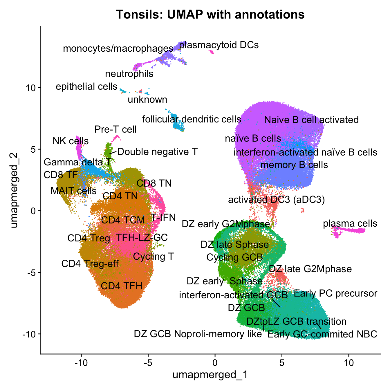
Save Final SEU object ( All cells)
out3 <- here("output",
            "RDS", "AllBatches_Final_Clusters_SEUs",
             paste0("G000231_Neeland_",tissue,".final_clusters.SEU.rds"))
#dir.create(out3)
if (!file.exists(out3)) {
  saveRDS(merged, file = out3)
}
Session Info
sessioninfo::session_info()─ Session info ───────────────────────────────────────────────────────────────
setting value
version R version 4.3.2 (2023-10-31)
os macOS Sonoma 14.6.1
system aarch64, darwin20
ui X11
language (EN)
collate en_US.UTF-8
ctype en_US.UTF-8
tz Australia/Melbourne
date 2024-09-23
pandoc 3.1.1 @ /Users/dixitgunjan/Desktop/RStudio.app/Contents/Resources/app/quarto/bin/tools/ (via rmarkdown)
─ Packages ───────────────────────────────────────────────────────────────────
package * version date (UTC) lib source
abind 1.4-5 2016-07-21 [1] CRAN (R 4.3.0)
AnnotationDbi * 1.64.1 2023-11-02 [1] Bioconductor
backports 1.4.1 2021-12-13 [1] CRAN (R 4.3.0)
Biobase * 2.62.0 2023-10-26 [1] Bioconductor
BiocGenerics * 0.48.1 2023-11-02 [1] Bioconductor
BiocManager 1.30.22 2023-08-08 [1] CRAN (R 4.3.0)
BiocStyle * 2.30.0 2023-10-26 [1] Bioconductor
Biostrings 2.70.2 2024-01-30 [1] Bioconductor 3.18 (R 4.3.2)
bit 4.0.5 2022-11-15 [1] CRAN (R 4.3.0)
bit64 4.0.5 2020-08-30 [1] CRAN (R 4.3.0)
bitops 1.0-7 2021-04-24 [1] CRAN (R 4.3.0)
blob 1.2.4 2023-03-17 [1] CRAN (R 4.3.0)
bslib 0.6.1 2023-11-28 [1] CRAN (R 4.3.1)
cachem 1.0.8 2023-05-01 [1] CRAN (R 4.3.0)
callr 3.7.5 2024-02-19 [1] CRAN (R 4.3.1)
cellranger 1.1.0 2016-07-27 [1] CRAN (R 4.3.0)
checkmate 2.3.1 2023-12-04 [1] CRAN (R 4.3.1)
cli 3.6.2 2023-12-11 [1] CRAN (R 4.3.1)
cluster 2.1.6 2023-12-01 [1] CRAN (R 4.3.1)
clustree * 0.5.1 2023-11-05 [1] CRAN (R 4.3.1)
codetools 0.2-19 2023-02-01 [1] CRAN (R 4.3.2)
colorspace 2.1-0 2023-01-23 [1] CRAN (R 4.3.0)
cowplot 1.1.3 2024-01-22 [1] CRAN (R 4.3.1)
crayon 1.5.2 2022-09-29 [1] CRAN (R 4.3.0)
data.table * 1.15.0 2024-01-30 [1] CRAN (R 4.3.1)
DBI 1.2.2 2024-02-16 [1] CRAN (R 4.3.1)
DelayedArray 0.28.0 2023-11-06 [1] Bioconductor
deldir 2.0-2 2023-11-23 [1] CRAN (R 4.3.1)
digest 0.6.34 2024-01-11 [1] CRAN (R 4.3.1)
dotCall64 1.1-1 2023-11-28 [1] CRAN (R 4.3.1)
dplyr * 1.1.4 2023-11-17 [1] CRAN (R 4.3.1)
edgeR * 4.0.16 2024-02-20 [1] Bioconductor 3.18 (R 4.3.2)
ellipsis 0.3.2 2021-04-29 [1] CRAN (R 4.3.0)
evaluate 0.23 2023-11-01 [1] CRAN (R 4.3.1)
fansi 1.0.6 2023-12-08 [1] CRAN (R 4.3.1)
farver 2.1.1 2022-07-06 [1] CRAN (R 4.3.0)
fastDummies 1.7.3 2023-07-06 [1] CRAN (R 4.3.0)
fastmap 1.1.1 2023-02-24 [1] CRAN (R 4.3.0)
fitdistrplus 1.1-11 2023-04-25 [1] CRAN (R 4.3.0)
forcats * 1.0.0 2023-01-29 [1] CRAN (R 4.3.0)
fs 1.6.3 2023-07-20 [1] CRAN (R 4.3.0)
future 1.33.1 2023-12-22 [1] CRAN (R 4.3.1)
future.apply 1.11.1 2023-12-21 [1] CRAN (R 4.3.1)
generics 0.1.3 2022-07-05 [1] CRAN (R 4.3.0)
GenomeInfoDb 1.38.6 2024-02-10 [1] Bioconductor 3.18 (R 4.3.2)
GenomeInfoDbData 1.2.11 2024-02-27 [1] Bioconductor
GenomicRanges 1.54.1 2023-10-30 [1] Bioconductor
getPass 0.2-4 2023-12-10 [1] CRAN (R 4.3.1)
ggforce 0.4.2 2024-02-19 [1] CRAN (R 4.3.1)
ggplot2 * 3.5.0 2024-02-23 [1] CRAN (R 4.3.1)
ggraph * 2.1.0 2022-10-09 [1] CRAN (R 4.3.0)
ggrepel 0.9.5 2024-01-10 [1] CRAN (R 4.3.1)
ggridges 0.5.6 2024-01-23 [1] CRAN (R 4.3.1)
git2r 0.33.0 2023-11-26 [1] CRAN (R 4.3.1)
globals 0.16.2 2022-11-21 [1] CRAN (R 4.3.0)
glue * 1.7.0 2024-01-09 [1] CRAN (R 4.3.1)
goftest 1.2-3 2021-10-07 [1] CRAN (R 4.3.0)
graphlayouts 1.1.0 2024-01-19 [1] CRAN (R 4.3.1)
gridExtra 2.3 2017-09-09 [1] CRAN (R 4.3.0)
gtable 0.3.4 2023-08-21 [1] CRAN (R 4.3.0)
here * 1.0.1 2020-12-13 [1] CRAN (R 4.3.0)
highr 0.10 2022-12-22 [1] CRAN (R 4.3.0)
hms 1.1.3 2023-03-21 [1] CRAN (R 4.3.0)
htmltools 0.5.7 2023-11-03 [1] CRAN (R 4.3.1)
htmlwidgets 1.6.4 2023-12-06 [1] CRAN (R 4.3.1)
httpuv 1.6.14 2024-01-26 [1] CRAN (R 4.3.1)
httr 1.4.7 2023-08-15 [1] CRAN (R 4.3.0)
ica 1.0-3 2022-07-08 [1] CRAN (R 4.3.0)
igraph 2.0.2 2024-02-17 [1] CRAN (R 4.3.1)
IRanges * 2.36.0 2023-10-26 [1] Bioconductor
irlba 2.3.5.1 2022-10-03 [1] CRAN (R 4.3.2)
jquerylib 0.1.4 2021-04-26 [1] CRAN (R 4.3.0)
jsonlite 1.8.8 2023-12-04 [1] CRAN (R 4.3.1)
kableExtra * 1.4.0 2024-01-24 [1] CRAN (R 4.3.1)
KEGGREST 1.42.0 2023-10-26 [1] Bioconductor
KernSmooth 2.23-22 2023-07-10 [1] CRAN (R 4.3.2)
knitr 1.45 2023-10-30 [1] CRAN (R 4.3.1)
labeling 0.4.3 2023-08-29 [1] CRAN (R 4.3.0)
later 1.3.2 2023-12-06 [1] CRAN (R 4.3.1)
lattice 0.22-5 2023-10-24 [1] CRAN (R 4.3.1)
lazyeval 0.2.2 2019-03-15 [1] CRAN (R 4.3.0)
leiden 0.4.3.1 2023-11-17 [1] CRAN (R 4.3.1)
lifecycle 1.0.4 2023-11-07 [1] CRAN (R 4.3.1)
limma * 3.58.1 2023-11-02 [1] Bioconductor
listenv 0.9.1 2024-01-29 [1] CRAN (R 4.3.1)
lmtest 0.9-40 2022-03-21 [1] CRAN (R 4.3.0)
locfit 1.5-9.8 2023-06-11 [1] CRAN (R 4.3.0)
lubridate * 1.9.3 2023-09-27 [1] CRAN (R 4.3.1)
magrittr 2.0.3 2022-03-30 [1] CRAN (R 4.3.0)
MASS 7.3-60.0.1 2024-01-13 [1] CRAN (R 4.3.1)
Matrix 1.6-5 2024-01-11 [1] CRAN (R 4.3.1)
MatrixGenerics 1.14.0 2023-10-26 [1] Bioconductor
matrixStats 1.2.0 2023-12-11 [1] CRAN (R 4.3.1)
memoise 2.0.1 2021-11-26 [1] CRAN (R 4.3.0)
mime 0.12 2021-09-28 [1] CRAN (R 4.3.0)
miniUI 0.1.1.1 2018-05-18 [1] CRAN (R 4.3.0)
munsell 0.5.0 2018-06-12 [1] CRAN (R 4.3.0)
nlme 3.1-164 2023-11-27 [1] CRAN (R 4.3.1)
org.Hs.eg.db * 3.18.0 2024-02-27 [1] Bioconductor
paletteer 1.6.0 2024-01-21 [1] CRAN (R 4.3.1)
parallelly 1.37.0 2024-02-14 [1] CRAN (R 4.3.1)
patchwork * 1.2.0 2024-01-08 [1] CRAN (R 4.3.1)
pbapply 1.7-2 2023-06-27 [1] CRAN (R 4.3.0)
pillar 1.9.0 2023-03-22 [1] CRAN (R 4.3.0)
pkgconfig 2.0.3 2019-09-22 [1] CRAN (R 4.3.0)
plotly 4.10.4 2024-01-13 [1] CRAN (R 4.3.1)
plyr 1.8.9 2023-10-02 [1] CRAN (R 4.3.1)
png 0.1-8 2022-11-29 [1] CRAN (R 4.3.0)
polyclip 1.10-6 2023-09-27 [1] CRAN (R 4.3.1)
presto 1.0.0 2024-02-27 [1] Github (immunogenomics/presto@31dc97f)
prismatic 1.1.1 2022-08-15 [1] CRAN (R 4.3.0)
processx 3.8.3 2023-12-10 [1] CRAN (R 4.3.1)
progressr 0.14.0 2023-08-10 [1] CRAN (R 4.3.0)
promises 1.2.1 2023-08-10 [1] CRAN (R 4.3.0)
ps 1.7.6 2024-01-18 [1] CRAN (R 4.3.1)
purrr * 1.0.2 2023-08-10 [1] CRAN (R 4.3.0)
R6 2.5.1 2021-08-19 [1] CRAN (R 4.3.0)
RANN 2.6.1 2019-01-08 [1] CRAN (R 4.3.0)
RColorBrewer * 1.1-3 2022-04-03 [1] CRAN (R 4.3.0)
Rcpp 1.0.12 2024-01-09 [1] CRAN (R 4.3.1)
RcppAnnoy 0.0.22 2024-01-23 [1] CRAN (R 4.3.1)
RcppHNSW 0.6.0 2024-02-04 [1] CRAN (R 4.3.1)
RCurl 1.98-1.14 2024-01-09 [1] CRAN (R 4.3.1)
readr * 2.1.5 2024-01-10 [1] CRAN (R 4.3.1)
readxl * 1.4.3 2023-07-06 [1] CRAN (R 4.3.0)
rematch2 2.1.2 2020-05-01 [1] CRAN (R 4.3.0)
reshape2 1.4.4 2020-04-09 [1] CRAN (R 4.3.0)
reticulate 1.35.0 2024-01-31 [1] CRAN (R 4.3.1)
rlang 1.1.3 2024-01-10 [1] CRAN (R 4.3.1)
rmarkdown 2.25 2023-09-18 [1] CRAN (R 4.3.1)
ROCR 1.0-11 2020-05-02 [1] CRAN (R 4.3.0)
rprojroot 2.0.4 2023-11-05 [1] CRAN (R 4.3.1)
RSpectra 0.16-1 2022-04-24 [1] CRAN (R 4.3.0)
RSQLite 2.3.5 2024-01-21 [1] CRAN (R 4.3.1)
rstudioapi 0.15.0 2023-07-07 [1] CRAN (R 4.3.0)
Rtsne 0.17 2023-12-07 [1] CRAN (R 4.3.1)
S4Arrays 1.2.0 2023-10-26 [1] Bioconductor
S4Vectors * 0.40.2 2023-11-25 [1] Bioconductor 3.18 (R 4.3.2)
sass 0.4.8 2023-12-06 [1] CRAN (R 4.3.1)
scales 1.3.0 2023-11-28 [1] CRAN (R 4.3.1)
scattermore 1.2 2023-06-12 [1] CRAN (R 4.3.0)
sctransform 0.4.1 2023-10-19 [1] CRAN (R 4.3.1)
sessioninfo 1.2.2 2021-12-06 [1] CRAN (R 4.3.0)
Seurat * 5.0.1.9009 2024-02-28 [1] Github (satijalab/seurat@6a3ef5e)
SeuratObject * 5.0.1 2023-11-17 [1] CRAN (R 4.3.1)
shiny 1.8.0 2023-11-17 [1] CRAN (R 4.3.1)
SingleCellExperiment 1.24.0 2023-11-06 [1] Bioconductor
sp * 2.1-3 2024-01-30 [1] CRAN (R 4.3.1)
spam 2.10-0 2023-10-23 [1] CRAN (R 4.3.1)
SparseArray 1.2.4 2024-02-10 [1] Bioconductor 3.18 (R 4.3.2)
spatstat.data 3.0-4 2024-01-15 [1] CRAN (R 4.3.1)
spatstat.explore 3.2-6 2024-02-01 [1] CRAN (R 4.3.1)
spatstat.geom 3.2-8 2024-01-26 [1] CRAN (R 4.3.1)
spatstat.random 3.2-2 2023-11-29 [1] CRAN (R 4.3.1)
spatstat.sparse 3.0-3 2023-10-24 [1] CRAN (R 4.3.1)
spatstat.utils 3.0-4 2023-10-24 [1] CRAN (R 4.3.1)
speckle * 1.2.0 2023-10-26 [1] Bioconductor
statmod 1.5.0 2023-01-06 [1] CRAN (R 4.3.0)
stringi 1.8.3 2023-12-11 [1] CRAN (R 4.3.1)
stringr * 1.5.1 2023-11-14 [1] CRAN (R 4.3.1)
SummarizedExperiment 1.32.0 2023-11-06 [1] Bioconductor
survival 3.5-8 2024-02-14 [1] CRAN (R 4.3.1)
svglite 2.1.3 2023-12-08 [1] CRAN (R 4.3.1)
systemfonts 1.0.5 2023-10-09 [1] CRAN (R 4.3.1)
tensor 1.5 2012-05-05 [1] CRAN (R 4.3.0)
tibble * 3.2.1 2023-03-20 [1] CRAN (R 4.3.0)
tidygraph 1.3.1 2024-01-30 [1] CRAN (R 4.3.1)
tidyr * 1.3.1 2024-01-24 [1] CRAN (R 4.3.1)
tidyselect 1.2.0 2022-10-10 [1] CRAN (R 4.3.0)
tidyverse * 2.0.0 2023-02-22 [1] CRAN (R 4.3.0)
timechange 0.3.0 2024-01-18 [1] CRAN (R 4.3.1)
tweenr 2.0.3 2024-02-26 [1] CRAN (R 4.3.1)
tzdb 0.4.0 2023-05-12 [1] CRAN (R 4.3.0)
utf8 1.2.4 2023-10-22 [1] CRAN (R 4.3.1)
uwot 0.1.16 2023-06-29 [1] CRAN (R 4.3.0)
vctrs 0.6.5 2023-12-01 [1] CRAN (R 4.3.1)
viridis 0.6.5 2024-01-29 [1] CRAN (R 4.3.1)
viridisLite 0.4.2 2023-05-02 [1] CRAN (R 4.3.0)
whisker 0.4.1 2022-12-05 [1] CRAN (R 4.3.0)
withr 3.0.0 2024-01-16 [1] CRAN (R 4.3.1)
workflowr * 1.7.1 2023-08-23 [1] CRAN (R 4.3.0)
xfun 0.42 2024-02-08 [1] CRAN (R 4.3.1)
xml2 1.3.6 2023-12-04 [1] CRAN (R 4.3.1)
xtable 1.8-4 2019-04-21 [1] CRAN (R 4.3.0)
XVector 0.42.0 2023-10-26 [1] Bioconductor
yaml 2.3.8 2023-12-11 [1] CRAN (R 4.3.1)
zlibbioc 1.48.0 2023-10-26 [1] Bioconductor
zoo 1.8-12 2023-04-13 [1] CRAN (R 4.3.0)
[1] /Library/Frameworks/R.framework/Versions/4.3-arm64/Resources/library
──────────────────────────────────────────────────────────────────────────────
sessionInfo()R version 4.3.2 (2023-10-31)
Platform: aarch64-apple-darwin20 (64-bit)
Running under: macOS Sonoma 14.6.1
Matrix products: default
BLAS: /Library/Frameworks/R.framework/Versions/4.3-arm64/Resources/lib/libRblas.0.dylib
LAPACK: /Library/Frameworks/R.framework/Versions/4.3-arm64/Resources/lib/libRlapack.dylib; LAPACK version 3.11.0
locale:
[1] en_US.UTF-8/en_US.UTF-8/en_US.UTF-8/C/en_US.UTF-8/en_US.UTF-8
time zone: Australia/Melbourne
tzcode source: internal
attached base packages:
[1] stats4 stats graphics grDevices utils datasets methods
[8] base
other attached packages:
[1] readxl_1.4.3 org.Hs.eg.db_3.18.0 AnnotationDbi_1.64.1
[4] IRanges_2.36.0 S4Vectors_0.40.2 Biobase_2.62.0
[7] BiocGenerics_0.48.1 speckle_1.2.0 edgeR_4.0.16
[10] limma_3.58.1 patchwork_1.2.0 data.table_1.15.0
[13] RColorBrewer_1.1-3 kableExtra_1.4.0 clustree_0.5.1
[16] ggraph_2.1.0 Seurat_5.0.1.9009 SeuratObject_5.0.1
[19] sp_2.1-3 glue_1.7.0 here_1.0.1
[22] lubridate_1.9.3 forcats_1.0.0 stringr_1.5.1
[25] dplyr_1.1.4 purrr_1.0.2 readr_2.1.5
[28] tidyr_1.3.1 tibble_3.2.1 ggplot2_3.5.0
[31] tidyverse_2.0.0 BiocStyle_2.30.0 workflowr_1.7.1
loaded via a namespace (and not attached):
[1] fs_1.6.3 matrixStats_1.2.0
[3] spatstat.sparse_3.0-3 bitops_1.0-7
[5] httr_1.4.7 tools_4.3.2
[7] sctransform_0.4.1 backports_1.4.1
[9] utf8_1.2.4 R6_2.5.1
[11] lazyeval_0.2.2 uwot_0.1.16
[13] withr_3.0.0 gridExtra_2.3
[15] progressr_0.14.0 cli_3.6.2
[17] spatstat.explore_3.2-6 fastDummies_1.7.3
[19] prismatic_1.1.1 labeling_0.4.3
[21] sass_0.4.8 spatstat.data_3.0-4
[23] ggridges_0.5.6 pbapply_1.7-2
[25] systemfonts_1.0.5 svglite_2.1.3
[27] sessioninfo_1.2.2 parallelly_1.37.0
[29] rstudioapi_0.15.0 RSQLite_2.3.5
[31] generics_0.1.3 ica_1.0-3
[33] spatstat.random_3.2-2 Matrix_1.6-5
[35] fansi_1.0.6 abind_1.4-5
[37] lifecycle_1.0.4 whisker_0.4.1
[39] yaml_2.3.8 SummarizedExperiment_1.32.0
[41] SparseArray_1.2.4 Rtsne_0.17
[43] paletteer_1.6.0 grid_4.3.2
[45] blob_1.2.4 promises_1.2.1
[47] crayon_1.5.2 miniUI_0.1.1.1
[49] lattice_0.22-5 cowplot_1.1.3
[51] KEGGREST_1.42.0 pillar_1.9.0
[53] knitr_1.45 GenomicRanges_1.54.1
[55] future.apply_1.11.1 codetools_0.2-19
[57] leiden_0.4.3.1 getPass_0.2-4
[59] vctrs_0.6.5 png_0.1-8
[61] spam_2.10-0 cellranger_1.1.0
[63] gtable_0.3.4 rematch2_2.1.2
[65] cachem_1.0.8 xfun_0.42
[67] S4Arrays_1.2.0 mime_0.12
[69] tidygraph_1.3.1 survival_3.5-8
[71] SingleCellExperiment_1.24.0 statmod_1.5.0
[73] ellipsis_0.3.2 fitdistrplus_1.1-11
[75] ROCR_1.0-11 nlme_3.1-164
[77] bit64_4.0.5 RcppAnnoy_0.0.22
[79] GenomeInfoDb_1.38.6 rprojroot_2.0.4
[81] bslib_0.6.1 irlba_2.3.5.1
[83] KernSmooth_2.23-22 colorspace_2.1-0
[85] DBI_1.2.2 tidyselect_1.2.0
[87] processx_3.8.3 bit_4.0.5
[89] compiler_4.3.2 git2r_0.33.0
[91] xml2_1.3.6 DelayedArray_0.28.0
[93] plotly_4.10.4 checkmate_2.3.1
[95] scales_1.3.0 lmtest_0.9-40
[97] callr_3.7.5 digest_0.6.34
[99] goftest_1.2-3 spatstat.utils_3.0-4
[101] presto_1.0.0 rmarkdown_2.25
[103] XVector_0.42.0 htmltools_0.5.7
[105] pkgconfig_2.0.3 MatrixGenerics_1.14.0
[107] highr_0.10 fastmap_1.1.1
[109] rlang_1.1.3 htmlwidgets_1.6.4
[111] shiny_1.8.0 farver_2.1.1
[113] jquerylib_0.1.4 zoo_1.8-12
[115] jsonlite_1.8.8 RCurl_1.98-1.14
[117] magrittr_2.0.3 GenomeInfoDbData_1.2.11
[119] dotCall64_1.1-1 munsell_0.5.0
[121] Rcpp_1.0.12 viridis_0.6.5
[123] reticulate_1.35.0 stringi_1.8.3
[125] zlibbioc_1.48.0 MASS_7.3-60.0.1
[127] plyr_1.8.9 parallel_4.3.2
[129] listenv_0.9.1 ggrepel_0.9.5
[131] deldir_2.0-2 Biostrings_2.70.2
[133] graphlayouts_1.1.0 splines_4.3.2
[135] tensor_1.5 hms_1.1.3
[137] locfit_1.5-9.8 ps_1.7.6
[139] igraph_2.0.2 spatstat.geom_3.2-8
[141] RcppHNSW_0.6.0 reshape2_1.4.4
[143] evaluate_0.23 BiocManager_1.30.22
[145] tzdb_0.4.0 tweenr_2.0.3
[147] httpuv_1.6.14 RANN_2.6.1
[149] polyclip_1.10-6 future_1.33.1
[151] scattermore_1.2 ggforce_0.4.2
[153] xtable_1.8-4 RSpectra_0.16-1
[155] later_1.3.2 viridisLite_0.4.2
[157] memoise_2.0.1 cluster_2.1.6
[159] timechange_0.3.0 globals_0.16.2