Tonsils
Clustering and Marker gene analysis
Gunjan Dixit
July 26, 2024
Last updated: 2024-07-26
Checks: 6 1
Knit directory: paed-airway-allTissues/
This reproducible R Markdown analysis was created with workflowr (version 1.7.1). The Checks tab describes the reproducibility checks that were applied when the results were created. The Past versions tab lists the development history.
The R Markdown file has unstaged changes. To know which version of
the R Markdown file created these results, you’ll want to first commit
it to the Git repo. If you’re still working on the analysis, you can
ignore this warning. When you’re finished, you can run
wflow_publish to commit the R Markdown file and build the
HTML.
Great job! The global environment was empty. Objects defined in the global environment can affect the analysis in your R Markdown file in unknown ways. For reproduciblity it’s best to always run the code in an empty environment.
The command set.seed(20230811) was run prior to running
the code in the R Markdown file. Setting a seed ensures that any results
that rely on randomness, e.g. subsampling or permutations, are
reproducible.
Great job! Recording the operating system, R version, and package versions is critical for reproducibility.
Nice! There were no cached chunks for this analysis, so you can be confident that you successfully produced the results during this run.
Great job! Using relative paths to the files within your workflowr project makes it easier to run your code on other machines.
Great! You are using Git for version control. Tracking code development and connecting the code version to the results is critical for reproducibility.
The results in this page were generated with repository version 649de68. See the Past versions tab to see a history of the changes made to the R Markdown and HTML files.
Note that you need to be careful to ensure that all relevant files for
the analysis have been committed to Git prior to generating the results
(you can use wflow_publish or
wflow_git_commit). workflowr only checks the R Markdown
file, but you know if there are other scripts or data files that it
depends on. Below is the status of the Git repository when the results
were generated:
Ignored files:
    Ignored:    .DS_Store
    Ignored:    .RData
    Ignored:    .Rhistory
    Ignored:    .Rproj.user/
    Ignored:    analysis/.DS_Store
    Ignored:    data/.DS_Store
    Ignored:    data/RDS/
    Ignored:    output/.DS_Store
    Ignored:    output/CSV/.DS_Store
    Ignored:    output/G000231_Neeland_batch1/
    Ignored:    output/G000231_Neeland_batch2_1/
    Ignored:    output/G000231_Neeland_batch2_2/
    Ignored:    output/G000231_Neeland_batch3/
    Ignored:    output/G000231_Neeland_batch4/
    Ignored:    output/G000231_Neeland_batch5/
    Ignored:    output/G000231_Neeland_batch9_1/
    Ignored:    output/RDS/
    Ignored:    output/plots/

Untracked files:
    Untracked:  VennDiagram.2024-07-24_11-48-08.297746.log
    Untracked:  VennDiagram.2024-07-24_12-25-12.854839.log
    Untracked:  VennDiagram.2024-07-24_12-25-22.005094.log
    Untracked:  VennDiagram.2024-07-24_12-29-34.757841.log
    Untracked:  analysis/03_Batch_Integration.Rmd
    Untracked:  analysis/Age_proportions.Rmd
    Untracked:  analysis/Age_proportions_AllBatches.Rmd
    Untracked:  analysis/Batch_Integration_&_Downstream_analysis.Rmd
    Untracked:  analysis/Batch_correction_&_Downstream.Rmd
    Untracked:  analysis/Cell_cycle_regression.Rmd
    Untracked:  analysis/Preprocessing_Batch1_Nasal_brushings.Rmd
    Untracked:  analysis/Preprocessing_Batch2_Tonsils.Rmd
    Untracked:  analysis/Preprocessing_Batch3_Adenoids.Rmd
    Untracked:  analysis/Preprocessing_Batch4_Bronchial_brushings.Rmd
    Untracked:  analysis/Preprocessing_Batch5_Nasal_brushings.Rmd
    Untracked:  analysis/Preprocessing_Batch6_BAL.Rmd
    Untracked:  analysis/Preprocessing_Batch7_Bronchial_brushings.Rmd
    Untracked:  analysis/Preprocessing_Batch8_Adenoids.Rmd
    Untracked:  analysis/Preprocessing_Batch9_Tonsils.Rmd
    Untracked:  analysis/VennDiagram.2024-07-24_11-54-23.569848.log
    Untracked:  analysis/VennDiagram.2024-07-24_11-55-06.582353.log
    Untracked:  analysis/VennDiagram.2024-07-24_12-28-47.017253.log
    Untracked:  analysis/VennDiagram.2024-07-24_12-33-05.913419.log
    Untracked:  analysis/VennDiagram.2024-07-24_13-42-31.593316.log
    Untracked:  analysis/cell_cycle_regression.R
    Untracked:  analysis/test.Rmd
    Untracked:  analysis/testing_age_all.Rmd
    Untracked:  data/Cell_labels_Mel/
    Untracked:  data/Cell_labels_Mel_v2/
    Untracked:  data/Hs.c2.cp.reactome.v7.1.entrez.rds
    Untracked:  data/Raw_feature_bc_matrix/
    Untracked:  data/celltypes_Mel_GD_v3.xlsx
    Untracked:  data/celltypes_Mel_GD_v4_no_dups.xlsx
    Untracked:  data/celltypes_Mel_modified.xlsx
    Untracked:  data/celltypes_Mel_v2.csv
    Untracked:  data/celltypes_Mel_v2.xlsx
    Untracked:  data/celltypes_Mel_v2_MN.xlsx
    Untracked:  data/celltypes_for_mel_MN.xlsx
    Untracked:  data/earlyAIR_sample_sheets_combined.xlsx
    Untracked:  output/CSV/Bronchial_brushings_Marker_gene_clusters.limmaTrendRNA_snn_res.0.4/
    Untracked:  stacked_barplot.png
    Untracked:  stacked_barplot_donor_id.png

Unstaged changes:
    Deleted:    02_QC_exploratoryPlots.Rmd
    Deleted:    02_QC_exploratoryPlots.html
    Modified:   analysis/00_AllBatches_overview.Rmd
    Modified:   analysis/01_QC_emptyDrops.Rmd
    Modified:   analysis/02_QC_exploratoryPlots.Rmd
    Modified:   analysis/Adenoids.Rmd
    Modified:   analysis/Age_modeling.Rmd
    Modified:   analysis/AllBatches_QCExploratory.Rmd
    Modified:   analysis/BAL.Rmd
    Modified:   analysis/Tonsils.Rmd
    Modified:   output/CSV/BAL_Marker_gene_clusters.limmaTrendRNA_snn_res.0.4/REACTOME-cluster-limma-c0.csv
    Modified:   output/CSV/BAL_Marker_gene_clusters.limmaTrendRNA_snn_res.0.4/REACTOME-cluster-limma-c1.csv
    Modified:   output/CSV/BAL_Marker_gene_clusters.limmaTrendRNA_snn_res.0.4/REACTOME-cluster-limma-c10.csv
    Modified:   output/CSV/BAL_Marker_gene_clusters.limmaTrendRNA_snn_res.0.4/REACTOME-cluster-limma-c11.csv
    Modified:   output/CSV/BAL_Marker_gene_clusters.limmaTrendRNA_snn_res.0.4/REACTOME-cluster-limma-c12.csv
    Modified:   output/CSV/BAL_Marker_gene_clusters.limmaTrendRNA_snn_res.0.4/REACTOME-cluster-limma-c13.csv
    Modified:   output/CSV/BAL_Marker_gene_clusters.limmaTrendRNA_snn_res.0.4/REACTOME-cluster-limma-c14.csv
    Modified:   output/CSV/BAL_Marker_gene_clusters.limmaTrendRNA_snn_res.0.4/REACTOME-cluster-limma-c15.csv
    Modified:   output/CSV/BAL_Marker_gene_clusters.limmaTrendRNA_snn_res.0.4/REACTOME-cluster-limma-c16.csv
    Modified:   output/CSV/BAL_Marker_gene_clusters.limmaTrendRNA_snn_res.0.4/REACTOME-cluster-limma-c17.csv
    Modified:   output/CSV/BAL_Marker_gene_clusters.limmaTrendRNA_snn_res.0.4/REACTOME-cluster-limma-c2.csv
    Modified:   output/CSV/BAL_Marker_gene_clusters.limmaTrendRNA_snn_res.0.4/REACTOME-cluster-limma-c3.csv
    Modified:   output/CSV/BAL_Marker_gene_clusters.limmaTrendRNA_snn_res.0.4/REACTOME-cluster-limma-c4.csv
    Modified:   output/CSV/BAL_Marker_gene_clusters.limmaTrendRNA_snn_res.0.4/REACTOME-cluster-limma-c5.csv
    Modified:   output/CSV/BAL_Marker_gene_clusters.limmaTrendRNA_snn_res.0.4/REACTOME-cluster-limma-c6.csv
    Modified:   output/CSV/BAL_Marker_gene_clusters.limmaTrendRNA_snn_res.0.4/REACTOME-cluster-limma-c7.csv
    Modified:   output/CSV/BAL_Marker_gene_clusters.limmaTrendRNA_snn_res.0.4/REACTOME-cluster-limma-c8.csv
    Modified:   output/CSV/BAL_Marker_gene_clusters.limmaTrendRNA_snn_res.0.4/REACTOME-cluster-limma-c9.csv
    Modified:   output/CSV/BAL_Marker_gene_clusters.limmaTrendRNA_snn_res.0.4/up-cluster-limma-c0.csv
    Modified:   output/CSV/BAL_Marker_gene_clusters.limmaTrendRNA_snn_res.0.4/up-cluster-limma-c1.csv
    Modified:   output/CSV/BAL_Marker_gene_clusters.limmaTrendRNA_snn_res.0.4/up-cluster-limma-c10.csv
    Modified:   output/CSV/BAL_Marker_gene_clusters.limmaTrendRNA_snn_res.0.4/up-cluster-limma-c11.csv
    Modified:   output/CSV/BAL_Marker_gene_clusters.limmaTrendRNA_snn_res.0.4/up-cluster-limma-c12.csv
    Modified:   output/CSV/BAL_Marker_gene_clusters.limmaTrendRNA_snn_res.0.4/up-cluster-limma-c13.csv
    Modified:   output/CSV/BAL_Marker_gene_clusters.limmaTrendRNA_snn_res.0.4/up-cluster-limma-c14.csv
    Modified:   output/CSV/BAL_Marker_gene_clusters.limmaTrendRNA_snn_res.0.4/up-cluster-limma-c15.csv
    Modified:   output/CSV/BAL_Marker_gene_clusters.limmaTrendRNA_snn_res.0.4/up-cluster-limma-c16.csv
    Modified:   output/CSV/BAL_Marker_gene_clusters.limmaTrendRNA_snn_res.0.4/up-cluster-limma-c17.csv
    Modified:   output/CSV/BAL_Marker_gene_clusters.limmaTrendRNA_snn_res.0.4/up-cluster-limma-c2.csv
    Modified:   output/CSV/BAL_Marker_gene_clusters.limmaTrendRNA_snn_res.0.4/up-cluster-limma-c3.csv
    Modified:   output/CSV/BAL_Marker_gene_clusters.limmaTrendRNA_snn_res.0.4/up-cluster-limma-c4.csv
    Modified:   output/CSV/BAL_Marker_gene_clusters.limmaTrendRNA_snn_res.0.4/up-cluster-limma-c5.csv
    Modified:   output/CSV/BAL_Marker_gene_clusters.limmaTrendRNA_snn_res.0.4/up-cluster-limma-c6.csv
    Modified:   output/CSV/BAL_Marker_gene_clusters.limmaTrendRNA_snn_res.0.4/up-cluster-limma-c7.csv
    Modified:   output/CSV/BAL_Marker_gene_clusters.limmaTrendRNA_snn_res.0.4/up-cluster-limma-c8.csv
    Modified:   output/CSV/BAL_Marker_gene_clusters.limmaTrendRNA_snn_res.0.4/up-cluster-limma-c9.csv
Note that any generated files, e.g. HTML, png, CSS, etc., are not included in this status report because it is ok for generated content to have uncommitted changes.
These are the previous versions of the repository in which changes were
made to the R Markdown (analysis/Tonsils.Rmd) and HTML
(docs/Tonsils.html) files. If you’ve configured a remote
Git repository (see ?wflow_git_remote), click on the
hyperlinks in the table below to view the files as they were in that
past version.
| File | Version | Author | Date | Message |
|---|---|---|---|---|
| Rmd | 649de68 | Gunjan Dixit | 2024-07-19 | Added corresponding Azimuth reference plots |
| html | 649de68 | Gunjan Dixit | 2024-07-19 | Added corresponding Azimuth reference plots |
| Rmd | 8b388e7 | Gunjan Dixit | 2024-07-17 | Updated Adenoid/Tonsils Tcell & GC reclustering |
| html | 8b388e7 | Gunjan Dixit | 2024-07-17 | Updated Adenoid/Tonsils Tcell & GC reclustering |
| Rmd | c20f60f | Gunjan Dixit | 2024-07-08 | Updated marker gene dot plots |
| html | c20f60f | Gunjan Dixit | 2024-07-08 | Updated marker gene dot plots |
| Rmd | 77c742e | Gunjan Dixit | 2024-06-26 | Updated RMarkdown files of all Tissues |
| html | 77c742e | Gunjan Dixit | 2024-06-26 | Updated RMarkdown files of all Tissues |
| Rmd | f27efbf | Gunjan Dixit | 2024-06-25 | Updated reclustering of Tonsils/Adenoids |
| html | f27efbf | Gunjan Dixit | 2024-06-25 | Updated reclustering of Tonsils/Adenoids |
| Rmd | 5aee5dd | Gunjan Dixit | 2024-05-07 | Modified Adenoids/Tonsils analysis |
| html | 5aee5dd | Gunjan Dixit | 2024-05-07 | Modified Adenoids/Tonsils analysis |
| Rmd | 320ccbd | Gunjan Dixit | 2024-05-01 | Modified/Annotated RMarkdown files |
| html | 320ccbd | Gunjan Dixit | 2024-05-01 | Modified/Annotated RMarkdown files |
| html | f460bd0 | Gunjan Dixit | 2024-04-26 | Modified BAL |
| html | e176340 | Gunjan Dixit | 2024-04-26 | Build site. |
| Rmd | 9492583 | Gunjan Dixit | 2024-04-26 | Added new analysis |
| html | 9492583 | Gunjan Dixit | 2024-04-26 | Added new analysis |
Introduction
This Rmarkdown file loads and analyzes the batch-integrated/merged
Seurat object for Tonsils (Batch2 and Batch9). It
performs clustering at various resolutions ranging from 0-1, followed by
visualization of identified clusters and Broad Level 3 cell labels on
UMAP. Next, the FindAllMarkers function is used to perform
marker gene analysis to identify marker genes for each cluster. The top
marker gene is visualized using FeaturePlot,
ViolinPlot and Heatmap. The identified marker
genes are stored in CSV format for each cluster at the optimum
resolution identified using clustree function.
Load libraries
suppressPackageStartupMessages({
  library(BiocStyle)
  library(tidyverse)
  library(here)
  library(dplyr)
  library(Seurat)
  library(clustree)
  library(kableExtra)
  library(RColorBrewer)
  library(data.table)
  library(ggplot2)
  library(patchwork)
})
Load Input data
Load merged object (batch corrected/integrated) for the tissue.
tissue <- "Tonsils"
out <- here("output/RDS/AllBatches_Harmony_SEUs/G000231_Neeland_Tonsils_batchCorrection.Harmony.clusters.SEU.rds")
merged_obj <- readRDS(out)
merged_obj
An object of class Seurat
17566 features across 141705 samples within 1 assay
Active assay: RNA (17566 features, 2000 variable features)
5 layers present: counts.G000231_batch2, counts.G000231_batch9, scale.data, data.G000231_batch2, data.G000231_batch9
4 dimensional reductions calculated: pca, umap.unintegrated, harmony, umap.harmonyClustering
Clustering is done on the “harmony” or batch integrated reduction at resolutions ranging from 0-1.
out1 <- here("output",
            "RDS", "AllBatches_Clustering_SEUs",
             paste0("G000231_Neeland_",tissue,".Clusters.SEU.rds"))
#dir.create(out1)

resolutions <- seq(0.1, 1, by = 0.1)
if (!file.exists(out1)) {
merged_obj <- FindNeighbors(merged_obj, reduction = "harmony", dims = 1:30)
merged_obj <- FindClusters(merged_obj, resolution = seq(0.1, 1, by = 0.1), algorithm = 3)
saveRDS(merged_obj, file = out1)
} else {
    merged_obj <- readRDS(out1)
}
The clustree function is used to visualize the
clustering at different resolutions to identify the most optimum
resolution.
clustree(merged_obj, prefix = "RNA_snn_res.")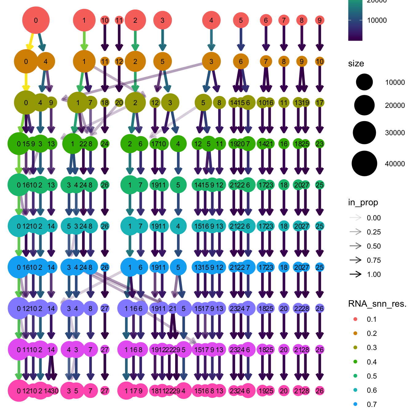
| Version | Author | Date |
|---|---|---|
| 320ccbd | Gunjan Dixit | 2024-05-01 |
Based on the clustering tree, we chose an intermediate/optimum resolution where the clustering results are the most stable, with the least amount of shuffling cells.
opt_res <- "RNA_snn_res.0.4"
n <- nlevels(merged_obj$RNA_snn_res.0.4)
merged_obj$RNA_snn_res.0.4 <- factor(merged_obj$RNA_snn_res.0.4, levels = seq(0,n-1))
merged_obj$seurat_clusters <- NULL
merged_obj$cluster <- merged_obj$RNA_snn_res.0.4
Idents(merged_obj) <- merged_obj$cluster
UMAP after clustering
Defining colours for each cell-type to be consistent with other age-related/cell type composition plots.
my_colors <- c(
  "B cells" = "steelblue",
  "CD4 T cells" = "brown",
  "Double negative T cells" = "gold",
  "CD8 T cells" = "lightgreen",
  "Pre B/T cells" = "orchid",
  "Innate lymphoid cells" = "tan",
  "Natural Killer cells" = "blueviolet",
  "Macrophages" = "green4",
  "Cycling T cells" = "turquoise",
  "Dendritic cells" = "grey80",
  "Gamma delta T cells" = "mediumvioletred",
  "Epithelial lineage" = "darkorange",
  "Granulocytes" = "olivedrab",
  "Fibroblast lineage" = "lavender",
  "None" = "white",
  "Monocytes" = "peachpuff",
  "Endothelial lineage" = "cadetblue",
  "SMG duct" = "lightpink",
  "Neuroendocrine" = "skyblue",
  "Doublet query/Other" = "#d62728"
)
# Define custom colors
custom_colors <- list()
colors_1 <- c(
  '#FFC312', '#C4E538', '#12CBC4', '#FDA7DF', '#ED4C67',
  "lavender", '#A3CB38', '#1289A7', '#D980FA', '#B53471',
  '#EE5A24', '#009432', '#0652DD', '#9980FA', '#833471',
  '#EA2027', '#006266', '#1B1464', '#5758BB', '#6F1E51'
)

colors_2 <- c(
  "darkorange", '#cc8e35', '#ffe119', '#4363d8', '#ffda79',
  '#911eb4', '#42d4f4', '#f032e6', '#bfef45', 'grey90',
  '#469990', '#dcbeff', '#9A6324', '#fffac8', '#800000',
  '#aaffc3', '#808000', '#ffd8b1', '#000075', '#a9a9a9'
)

custom_colors$discrete <- c(colors_1, colors_2)
UMAP displaying clusters at opt_res resolution and Broad
cell Labels Level 3.
p1 <- DimPlot(merged_obj, reduction = "umap.harmony", raster = FALSE ,repel = TRUE, label = TRUE,label.size = 3.5, group.by = opt_res) +  NoLegend()

p2 <- DimPlot(merged_obj, reduction = "umap.harmony", raster = FALSE, repel = TRUE, label = TRUE, label.size = 3.5, group.by = "Broad_cell_label_3") +
  scale_colour_manual(values = my_colors) +
  ggtitle(paste0(tissue, ": Batch Corrected UMAP"))


p1 / p2 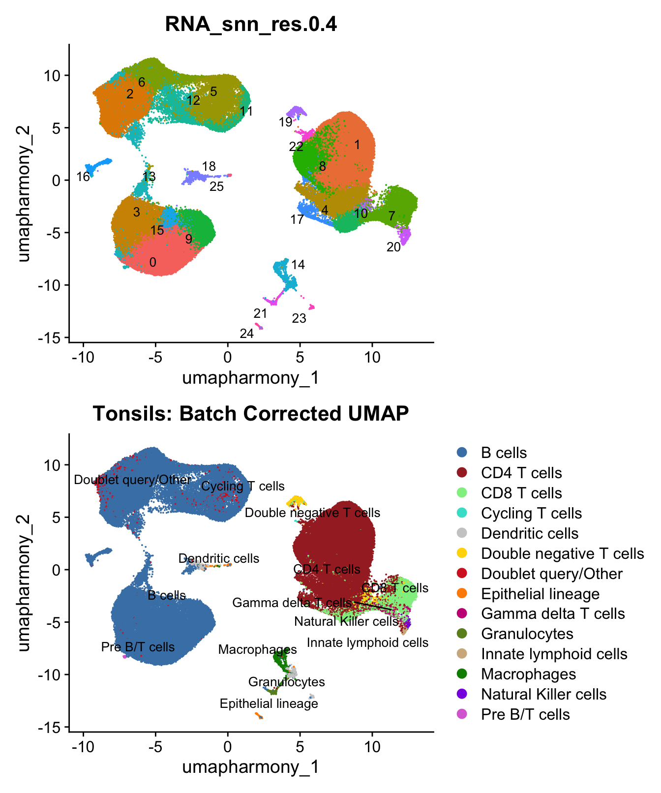
| Version | Author | Date |
|---|---|---|
| 320ccbd | Gunjan Dixit | 2024-05-01 |
p3 <- DimPlot(merged_obj, reduction = "umap.harmony", raster = FALSE, repel = TRUE, label = TRUE, label.size = 3.5, group.by = "predicted.celltype.l1") + NoLegend()
p3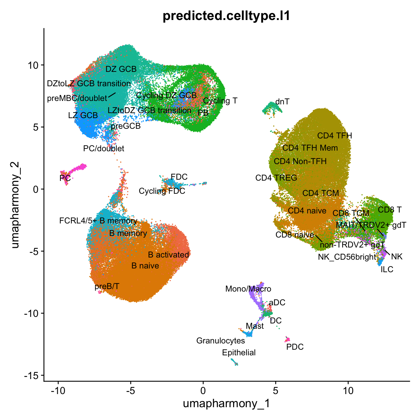
| Version | Author | Date |
|---|---|---|
| 5aee5dd | Gunjan Dixit | 2024-05-07 |
p4 <- DimPlot(merged_obj, reduction = "umap.harmony", raster = FALSE, repel = TRUE, label = TRUE, label.size = 3.5, group.by = "predicted.celltype.l2") + NoLegend()
p4
Warning: ggrepel: 44 unlabeled data points (too many overlaps). Consider
increasing max.overlaps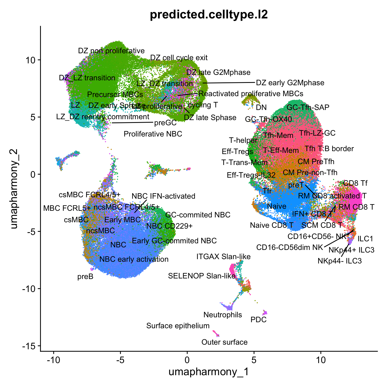
| Version | Author | Date |
|---|---|---|
| 5aee5dd | Gunjan Dixit | 2024-05-07 |
p1 <- merged_obj@meta.data %>%
  ggplot(aes(x = !!sym(opt_res),
             fill = !!sym(opt_res))) +
  geom_bar() +
  geom_text(aes(label = ..count..), stat = "count",
            vjust = -0.5, colour = "black", size = 2) +
  scale_y_log10() +
  theme(axis.text.x = element_text(angle = 90,
                                   vjust = 0.5,
                                   hjust = 1,
                                   size = 8)) +
  NoLegend() +
  labs(y = "No. Cells (log scale)")

p2 <- merged_obj@meta.data %>%
  dplyr::select(!!sym(opt_res), predicted.celltype.l1) %>%
  group_by(!!sym(opt_res), predicted.celltype.l1) %>%
  summarise(num = n()) %>%
  mutate(prop = num / sum(num)) %>%
  ggplot(aes(x = !!sym(opt_res), y = prop * 100,
             fill = predicted.celltype.l1)) +
  geom_bar(stat = "identity") +
  theme(axis.text.x = element_text(angle = 90,
                                   vjust = 0.5,
                                   hjust = 1,
                                   size = 8)) +
  labs(y = "% Cells", fill = "predicted.celltype.l1") +
  scale_fill_manual(values = custom_colors$discrete) #+
`summarise()` has grouped output by 'RNA_snn_res.0.4'. You can override using
the `.groups` argument. # paletteer::scale_fill_paletteer_d("ggsci::default_igv")
p3 <- merged_obj@meta.data %>%
dplyr::select(!!sym(opt_res), Broad_cell_label_3) %>%
group_by(!!sym(opt_res), Broad_cell_label_3) %>%
summarise(num = n()) %>%
mutate(prop = num / sum(num)) %>%
ggplot(aes(x = !!sym(opt_res), y = prop * 100,
fill = Broad_cell_label_3)) +
geom_bar(stat = "identity") +
theme(axis.text.x = element_text(angle = 90,
vjust = 0.5,
hjust = 1,
size = 8)) +
labs(y = "% Cells", fill = "Sample") +
scale_fill_manual(values = my_colors) `summarise()` has grouped output by 'RNA_snn_res.0.4'. You can override using
the `.groups` argument.# Combine the plots
(p1 / p2 / p3 ) & theme(legend.text = element_text(size = 8),
legend.key.size = unit(3, "mm"))
| Version | Author | Date |
|---|---|---|
| 5aee5dd | Gunjan Dixit | 2024-05-07 |
This table shows Azimuth Level 2 predicted cell types and their counts in each cluster in descending order.
cluster_ids <- sort(unique(merged_obj$cluster))
cluster_celltype_counts <- list()

for (cluster_id in cluster_ids) {
  cluster_data <- merged_obj@meta.data[merged_obj$cluster == cluster_id, ]
  table_counts <- table(cluster_data$predicted.celltype.l2)
  sorted_table <- table_counts[order(-table_counts)]
  cluster_celltype_counts[[as.character(cluster_id)]] <- sorted_table
}

cluster_celltype_counts
$`0`
NBC NBC early activation
15936 11582
ncsMBC Early GC-commited NBC
296 271
csMBC NBC IFN-activated
101 61
ncsMBC FCRL4/5+ GC-commited NBC
59 47
Early MBC preGC
42 26
MBC derived early PC precursor MBC FCRL5+
7 4
Precursor MBCs DZ_LZ transition
2 1
NBC CD229+
1
$`1`
Tfh-LZ-GC CM PreTfh GC-Tfh-SAP Tfh-Mem CM Pre-non-Tfh
8293 4291 3536 1622 1193
GC-Tfh-OX40 T-Eff-Mem Eff-Tregs-IL32 Naive Tfh T:B border
673 671 288 231 98
Eff-Tregs T-Trans-Mem T-helper CM CD8 T DN
82 76 39 30 24
SCM CD8 T cycling T Tfr CD8 Tf Naive CD8 T
21 11 8 2 2
RM CD8 T NBC Neutrophils NKp44+ ILC3 TCRVδ+ gd T
2 1 1 1 1
$`2`
DZ_LZ transition LZ LZ_DZ reentry commitment
13150 2097 298
Precursor MBCs preGC DZ non proliferative
243 87 54
NBC early activation NBC Early MBC
16 9 8
ncsMBC GC-commited NBC ncsMBC FCRL4/5+
5 4 3
csMBC NBC IFN-activated csMBC FCRL4/5+
2 2 1
Early GC-commited NBC
1
$`3`
csMBC NBC
2637 2283
ncsMBC FCRL4/5+ ncsMBC
2226 2215
csMBC FCRL4/5+ MBC FCRL5+
1385 1027
NBC early activation Early MBC
698 225
NBC IFN-activated Early GC-commited NBC
94 32
GC-commited NBC Precursor MBCs
26 23
preGC MBC derived early PC precursor
22 4
LZ_DZ reentry commitment DZ_LZ transition
3 2
NBC CD229+
1
$`4`
Naive CM Pre-non-Tfh CM PreTfh
8691 526 375
GC-Tfh-OX40 Tfh-LZ-GC Eff-Tregs-IL32
230 103 69
Naive CD8 T Tfr T-Eff-Mem
40 36 31
DN Eff-Tregs Tfh-Mem
30 26 10
cycling T SCM CD8 T T-Trans-Mem
8 4 3
TCRVδ+ gd T CM CD8 T NBC
3 2 2
NBC early activation GC-Tfh-SAP T-helper
2 1 1
$`5`
DZ late G2Mphase DZ late Sphase
2061 1304
DZ early Sphase Reactivated proliferative MBCs
724 723
DZ early G2Mphase LZ proliferative
447 402
LZ_DZ transition Precursor MBCs
392 360
csMBC DZ cell cycle exit
320 300
preGC DZ_LZ transition
208 202
NBC LZ_DZ reentry commitment
122 59
cycling T Early MBC
58 54
GC-commited NBC DZ non proliferative
44 35
LZ MBC derived early PC precursor
33 22
MBC FCRL5+ ncsMBC FCRL4/5+
8 8
cycling FDC csMBC FCRL4/5+
7 5
NBC IFN-activated PB
3 3
NBC early activation Early GC-commited NBC
2 1
GC-Tfh-OX40 ncsMBC
1 1
Proliferative NBC
1
$`6`
DZ non proliferative DZ_LZ transition DZ cell cycle exit
4522 1680 256
Precursor MBCs LZ DZ early Sphase
116 14 8
NBC preGC csMBC
5 4 2
DZ late G2Mphase NBC IFN-activated preB
2 2 1
$`7`
RM CD8 activated T RM CD8 T
1842 1220
CM CD8 T TCRVδ+ gd T
641 498
DN Naive
267 244
SCM CD8 T MAIT/CD161+TRDV2+ gd T-cells
236 205
CM Pre-non-Tfh CD8 Tf
193 130
Tfh-LZ-GC Naive CD8 T
126 107
IFN+ CD8 T ZNF683+ CD8 T
97 69
Eff-Tregs DC recruiters CD8 T
67 63
CM PreTfh T-helper
54 34
CD16-CD56+ NK Eff-Tregs-IL32
31 25
EM CD8 T CD16+CD56- NK
19 16
Tfh-Mem Tfr
11 7
CD16-CD56dim NK T-Trans-Mem
6 6
ILC1 csMBC
5 4
NKp44+ ILC3 GC-Tfh-OX40
4 3
GC-Tfh-SAP
3
$`8`
Tfh-Mem Eff-Tregs
1752 1354
Eff-Tregs-IL32 T-helper
832 662
Tfh-LZ-GC CM PreTfh
294 212
Naive GC-Tfh-OX40
205 182
CM Pre-non-Tfh T-Trans-Mem
144 102
T-Eff-Mem Tfr
63 35
GC-Tfh-SAP CM CD8 T
33 7
MAIT/CD161+TRDV2+ gd T-cells DN
7 4
NKp44+ ILC3 RM CD8 activated T
4 4
RM CD8 T SCM CD8 T
2 2
CD16+CD56- NK ILC1
1 1
MBC FCRL5+ Tfh T:B border
1 1
ZNF683+ CD8 T
1
$`9`
Early GC-commited NBC GC-commited NBC NBC
1809 1111 837
NBC early activation ncsMBC FCRL4/5+ ncsMBC
638 91 39
MBC FCRL5+ csMBC Early MBC
35 25 21
csMBC FCRL4/5+ Precursor MBCs LZ_DZ reentry commitment
15 12 6
NBC IFN-activated preGC NBC CD229+
4 4 3
DZ_LZ transition GC-Tfh-OX40 LZ
1 1 1
Naive
1
$`10`
Naive CD8 T Naive CM Pre-non-Tfh
2042 1472 53
SCM CD8 T CM PreTfh CM CD8 T
38 19 17
DN TCRVδ+ gd T Tfr
17 9 4
Eff-Tregs NBC early activation T-Trans-Mem
2 1 1
Tfh-LZ-GC
1
$`11`
DZ late Sphase DZ early G2Mphase
2483 723
DZ early Sphase LZ proliferative
31 26
Reactivated proliferative MBCs DZ late G2Mphase
10 8
LZ_DZ transition LZ
3 1
$`12`
DZ early Sphase DZ_LZ transition
1815 432
DZ non proliferative LZ
226 56
LZ_DZ reentry commitment DZ late Sphase
43 41
LZ proliferative DZ cell cycle exit
41 12
Precursor MBCs GC-commited NBC
8 3
DZ late G2Mphase preGC
2 2
Reactivated proliferative MBCs
2
$`13`
csMBC NBC
535 352
preGC DZ_LZ transition
295 265
ncsMBC FCRL4/5+ Precursor MBCs
138 135
Early MBC LZ_DZ reentry commitment
112 96
csMBC FCRL4/5+ LZ
95 87
DZ non proliferative GC-commited NBC
73 54
MBC FCRL5+ MBC derived early PC precursor
34 27
preB NBC early activation
14 9
DZ early Sphase NBC IFN-activated
7 6
DZ cell cycle exit Reactivated proliferative MBCs
5 3
LZ proliferative ncsMBC
2 2
cycling FDC Naive
1 1
Proliferative NBC
1
$`14`
SELENOP Slan-like ITGAX Slan-like C1Q Slan-like
653 209 197
DC2 DC5 DC1 precursor
111 103 90
MMP Slan-like aDC1 M1 Macrophages
81 65 48
aDC3 csMBC Monocytes
26 26 16
DC1 mature Mast preGC
15 12 8
Basal cells COL27A1+ FDC Crypt
4 3 3
DC4 IL7R DC MRC
3 3 3
FDC ncsMBC FCRL4/5+ RM CD8 activated T
2 2 2
CM Pre-non-Tfh CM PreTfh csMBC FCRL4/5+
1 1 1
Early GC-commited NBC Naive Neutrophils
1 1 1
PDC
1
$`15`
NBC IFN-activated NBC NBC early activation
987 478 116
ncsMBC GC-commited NBC Early GC-commited NBC
15 9 8
csMBC ncsMBC FCRL4/5+ Early MBC
7 7 2
Naive preGC
1 1
$`16`
IgG+ PC precursor preMature IgG+ PC
223 203
NBC Mature IgG+ PC
198 139
csMBC Mature IgA+ PC
110 95
MBC derived IgA+ PC IgD PC precursor
60 51
MBC derived early PC precursor IgM+ early PC precursor
22 21
preMature IgM+ PC PB committed early PC precursor
15 10
IgM+ PC precursor PB
8 7
preGC MBC derived IgG+ PC
4 3
Short lived IgM+ PC Mature IgM+ PC
3 1
MBC FCRL5+
1
$`17`
Naive CM Pre-non-Tfh Tfh-LZ-GC Naive CD8 T
467 320 108 95
Eff-Tregs CM PreTfh Eff-Tregs-IL32 IFN+ CD8 T
38 27 19 12
Tfh-Mem DN SCM CD8 T cycling T
7 3 3 2
NBC IFN-activated T-Eff-Mem T-Trans-Mem GC-Tfh-SAP
2 2 2 1
RM CD8 activated T
1
$`18`
FDC COL27A1+ FDC NBC
369 191 99
csMBC cycling FDC Crypt
48 45 41
Early MBC MRC DZ_LZ transition
41 41 27
preGC csMBC FCRL4/5+ ncsMBC FCRL4/5+
15 13 10
Tfh-LZ-GC Basal cells Naive
10 9 8
MBC FCRL5+ NBC early activation PDC
7 6 5
Precursor MBCs LZ_DZ reentry commitment SELENOP Slan-like
5 4 4
aDC1 CM PreTfh FDCSP epithelium
3 3 3
aDC3 CD14+CD55+ FDC FRC
2 2 2
GC-commited NBC M1 Macrophages ncsMBC
2 2 2
C1Q Slan-like CD8 Tf CM Pre-non-Tfh
1 1 1
DC5 DZ early Sphase LZ
1 1 1
Mast Mature IgA+ PC RM CD8 activated T
1 1 1
SCM CD8 T Surface epithelium T-helper
1 1 1
Tfh-Mem
1
$`19`
DN Naive CM CD8 T CM Pre-non-Tfh Eff-Tregs-IL32
822 63 22 13 11
SCM CD8 T Tfh-LZ-GC CM PreTfh cycling T CD8 Tf
9 8 5 4 2
TCRVδ+ gd T GC-Tfh-OX40 IFN+ CD8 T Naive CD8 T T-helper
2 1 1 1 1
Tfr
1
$`20`
CD16-CD56+ NK NKp44+ ILC3
247 180
ILC1 CD16-CD56dim NK
44 38
CD16+CD56- NK ZNF683+ CD8 T
34 32
TCRVδ+ gd T CM PreTfh
29 17
T-Trans-Mem CM Pre-non-Tfh
17 16
CM CD8 T MAIT/CD161+TRDV2+ gd T-cells
10 10
Naive DC recruiters CD8 T
9 5
EM CD8 T Tfh-LZ-GC
5 5
RM CD8 activated T DN
3 1
IFN+ CD8 T NKp44- ILC3
1 1
T-helper Tfh-Mem
1 1
$`21`
Neutrophils M1 Macrophages Early GC-commited NBC
376 89 16
NBC early activation NBC CM PreTfh
13 9 6
Monocytes Naive NBC IFN-activated
2 2 2
Tfh-LZ-GC C1Q Slan-like COL27A1+ FDC
2 1 1
csMBC DC5 FDC
1 1 1
ITGAX Slan-like Mast ncsMBC
1 1 1
ncsMBC FCRL4/5+ preGC
1 1
$`22`
Tfh-LZ-GC Tfh-Mem Naive GC-Tfh-SAP Eff-Tregs
110 78 74 21 14
cycling T Eff-Tregs-IL32 CM Pre-non-Tfh GC-Tfh-OX40 T-helper
10 9 6 6 6
CM PreTfh T-Eff-Mem Naive CD8 T NBC DN
5 5 3 3 2
CD8 Tf preT Tfr
1 1 1
$`23`
PDC NBC csMBC DC5 CM PreTfh DC2
184 4 3 2 1 1
$`24`
Outer surface Surface epithelium NBC
94 73 3
FDCSP epithelium NBC early activation
2 1
$`25`
Surface epithelium preGC FDC Crypt
68 29 27 4
NBC
1 Save batch corrected Object
out1 <- here("output",
            "RDS", "AllBatches_Clustering_SEUs",
             paste0("G000231_Neeland_",tissue,".Clusters.SEU.rds"))
#dir.create(out1)
saveRDS(merged_obj, file = out1)
Marker Gene Analysis
merged_obj <- JoinLayers(merged_obj)
paed.markers <- FindAllMarkers(merged_obj, only.pos = TRUE, min.pct = 0.25, logfc.threshold = 0.25)
Extracting top 5 genes per cluster for visualization. The ‘top5’ contains the top 5 genes with the highest weighted average avg_log2FC within each cluster and the ‘best.wilcox.gene.per.cluster’ contains the single best gene with the highest weighted average avg_log2FC for each cluster.
paed.markers %>%
    group_by(cluster) %>% unique() %>%
    top_n(n = 5, wt = avg_log2FC) -> top5

paed.markers %>%
    group_by(cluster) %>%
    slice_head(n=1) %>%
    pull(gene) -> best.wilcox.gene.per.cluster

best.wilcox.gene.per.cluster
[1] "IGHD" "MAF" "LMO2" "TNFRSF13B" "LEF1" "HMGB2"
[7] "AICDA" "CCL5" "MAF" "PHACTR1" "CD8A" "MKI67"
[13] "MCM4" "ACTB" "LYZ" "IFI44L" "MZB1" "IFI44L"
[19] "CLU" "GZMK" "TRDC" "ITGAX" "MYB" "CLEC4C"
[25] "S100A9" "WFDC2" Marker gene expression in clusters
This heatmap depicts the expression of top five genes in each cluster.
DoHeatmap(merged_obj, features = top5$gene) + NoLegend()
| Version | Author | Date |
|---|---|---|
| 320ccbd | Gunjan Dixit | 2024-05-01 |
Violin plot shows the expression of top marker gene per cluster.
VlnPlot(merged_obj, features=best.wilcox.gene.per.cluster, ncol = 2, raster = FALSE, pt.size = FALSE)
| Version | Author | Date |
|---|---|---|
| 320ccbd | Gunjan Dixit | 2024-05-01 |
Violin plot shows the expression of top marker gene per cluster and compares its expression in both batches.
plots <- VlnPlot(merged_obj, features = best.wilcox.gene.per.cluster, split.by = "batch_name", group.by = "Broad_cell_label_3",
    pt.size = 0, combine = FALSE, raster = FALSE, split.plot = TRUE)
The default behaviour of split.by has changed.
Separate violin plots are now plotted side-by-side.
To restore the old behaviour of a single split violin,
set split.plot = TRUE.
This message will be shown once per session.wrap_plots(plots = plots, ncol = 1)
| Version | Author | Date |
|---|---|---|
| 320ccbd | Gunjan Dixit | 2024-05-01 |
Feature plot shows the expression of top marker genes per cluster.
FeaturePlot(merged_obj,features=best.wilcox.gene.per.cluster, reduction = 'umap.harmony', raster = FALSE, ncol = 2)
| Version | Author | Date |
|---|---|---|
| 320ccbd | Gunjan Dixit | 2024-05-01 |
Extract markers for each cluster
This section extracts marker genes for each cluster and save them as a CSV file.
out_markers <- here("output",
            "CSV",
            paste(tissue,"_Marker_gene_clusters.",opt_res, sep = ""))

dir.create(out_markers, recursive = TRUE, showWarnings = FALSE)

for (cl in unique(paed.markers$cluster)) {
  cluster_data <- paed.markers %>% dplyr::filter(cluster == cl)
  file_name <- here(out_markers, paste0("G000231_Neeland_",tissue, "_cluster_", cl, ".csv"))
  write.csv(cluster_data, file = file_name)
}
Updated cell-type labels
cell_labels <- readxl::read_excel(here("data/Cell_labels_Mel/earlyAIR_tonsil_annotations_18.06.24.xlsx"))
new_cluster_names <- cell_labels %>%
  dplyr::select(cluster, annotation) %>%
  deframe()

merged_obj <- RenameIdents(merged_obj, new_cluster_names)
merged_obj@meta.data$cell_labels <- Idents(merged_obj)

p3 <- DimPlot(merged_obj, reduction = "umap.harmony", raster = FALSE, repel = TRUE, label = TRUE, label.size = 3.5) + ggtitle(paste0(tissue, ": UMAP with Updated cell types")) + NoLegend()

#p1
p3
| Version | Author | Date |
|---|---|---|
| f27efbf | Gunjan Dixit | 2024-06-25 |
merged_obj@meta.data %>%
  ggplot(aes(x = cell_labels, fill = cell_labels)) +
  geom_bar() +
  geom_text(aes(label = ..count..), stat = "count",
            vjust = -0.5, colour = "black", size = 2) +
  theme(axis.text.x = element_text(angle = 90, vjust = 0.5, hjust = 1)) +
  NoLegend() + ggtitle(paste0(tissue, " : Counts per cell-type"))
| Version | Author | Date |
|---|---|---|
| f27efbf | Gunjan Dixit | 2024-06-25 |
Reclustering T cell subtypes
Reclustering clusters 1, 4, 7, 8, 10, 17, 19, 20, 22
The marker genes for this reclustering can be found here-
Tonsils_Tcell_population_res.0.4
sub_clusters <- c(1, 4, 7, 8, 10, 17, 19, 20, 22)

idx <- which(merged_obj$cluster %in% sub_clusters)
paed_sub <- merged_obj[,idx]
paed_sub
An object of class Seurat
17566 features across 50340 samples within 1 assay
Active assay: RNA (17566 features, 2000 variable features)
3 layers present: data, counts, scale.data
4 dimensional reductions calculated: pca, umap.unintegrated, harmony, umap.harmony# Visualize the clustering results
DimPlot(paed_sub, reduction = "umap.harmony", group.by = "cluster", label = TRUE, label.size = 2.5, repel = TRUE, raster = FALSE )
| Version | Author | Date |
|---|---|---|
| f27efbf | Gunjan Dixit | 2024-06-25 |
paed_sub <- paed_sub %>%
  NormalizeData() %>%
  FindVariableFeatures() %>%
  ScaleData() %>%
  RunPCA()
Normalizing layer: countsFinding variable features for layer countsCentering and scaling data matrixWarning: Different features in new layer data than already exists for
scale.dataPC_ 1
Positive: MAF, TOX2, PDCD1, CXCR5, TIGIT, POU2AF1, ICOS, IL21, SRGN, IKZF3
FAM43A, GNG4, ST8SIA1, TRIM8, RTP5, KIAA1324, SMCO4, BCL6, CTSB, TOX
ZNF703, TBC1D4, CD4, ITM2A, RNF19A, CTLA4, KCNK5, STK39, SARDH, RAB27A
Negative: KLF2, VIM, RASGRP2, TXNIP, SELL, EMP3, NELL2, CCR7, LEF1, RIPOR2
TMSB10, PLAC8, SAMHD1, S1PR1, KLRK1, PDE3B, IL7R, SAMD3, TRABD2A, CD55
CD96, NOG, PECAM1, CD8A, MGAT4A, FLT3LG, ITGA6, ITGB7, RASSF3, RASA3
PC_ 2
Positive: ACTN1, LEF1, CCR7, NOG, TRABD2A, LTB, CD40LG, LDHB, RASGRP2, CD4
SATB1, ITGA6, FHIT, MAL, NOSIP, OBSCN, EDAR, SELL, TMEM272, CSGALNACT1
PDK1, FKBP5, EPHX2, IL7R, SULT1B1, IL6R, AIF1, LRRN3, CDK5R1, PLAC8
Negative: NKG7, CST7, CCL5, GZMA, GZMK, CCR5, EOMES, CXCR6, KLRD1, PRF1
SLAMF7, CCL4, GNLY, PLEK, MYO1F, KLRK1, APOBEC3G, CTSW, IL2RB, AHNAK
FGR, FASLG, CLDND1, CXCR3, CD300A, PRR5L, KLRG1, ZEB2, HOPX, LAG3
PC_ 3
Positive: NKG7, CCL5, GZMK, EOMES, FCRL6, KLRK1, KLRG1, CXCR4, SLAMF7, AOAH
GZMA, CST7, CD8A, KLRD1, PLEK, KLRC4, CXCR5, TRGC2, DKK3, PTGDR
PRR5L, FGR, ITM2C, KLRC3, SPRY2, CCL4, CTSW, RTP5, ST8SIA1, CNIH3
Negative: COL5A3, RORA, CCND2, CTLA4, F5, IL2RA, GBP2, TMSB10, FOXP3, ZC3H12D
PRDM1, DUSP16, IL1R1, SLAMF1, IL1R2, ADTRP, LAG3, BCL2, TMEM173, PIM2
CCR7, TNFRSF1B, TNFRSF4, CD4, IRF4, CCR6, SAMHD1, LTB, ADAM19, FURIN
PC_ 4
Positive: KLRB1, RGS1, CXCR6, GPR183, PRDM1, MAF, CSF1, ADAM19, COL5A3, CCR4
PYHIN1, NABP1, CCR6, CCR5, PHTF2, ATP2B4, GLIPR1, KLF6, CD4, RORA
NBEAL2, FOXP3, IL1R2, SYNE2, PCDH1, DUSP1, SLAMF1, DUSP16, AHNAK, MAP3K5
Negative: LEF1, GNG4, NUCB2, ACTN1, PECAM1, MYB, KLRK1, CD55, MT-CO2, BACH2
RIPOR2, CXXC5, RIN3, NELL2, SPN, MT-CO3, MT-ND4L, MT-ND4, CTSW, MT-ATP6
TRABD2A, CD200, CD248, PKM, XXYLT1, ENO1, MT-CYB, HSP90AB1, DGKZ, PTPN14
PC_ 5
Positive: GNLY, SH2D1B, TYROBP, FCER1G, ATP8B4, ITGAX, KLRC1, NCAM1, KLRF1, ITGAM
NCR1, TRDC, HOPX, IL18RAP, KIT, XCL2, KLRD1, KLRB1, FES, KLRC3
IL7R, DLL1, ZBTB16, TLE1, SPTSSB, FGR, CTSW, TNFRSF18, ID2, DOCK5
Negative: GZMK, EOMES, PTPN3, GZMA, SLAMF7, DTHD1, CCR5, CD8A, CCL5, CD27
CST7, CAV1, CCL4, ANXA2, DKK3, FASLG, MYB, LYST, PRDM8, AGAP1
PECAM1, MPP1, SH2D1A, KLRG1, MT2A, PHLDA1, TIGIT, FABP5, CLDND1, PLEK paed_sub <- RunUMAP(paed_sub, dims = 1:30, reduction = "pca", reduction.name = "umap.new")Warning: The default method for RunUMAP has changed from calling Python UMAP via reticulate to the R-native UWOT using the cosine metric
To use Python UMAP via reticulate, set umap.method to 'umap-learn' and metric to 'correlation'
This message will be shown once per session11:09:05 UMAP embedding parameters a = 0.9922 b = 1.11211:09:05 Read 50340 rows and found 30 numeric columns11:09:05 Using Annoy for neighbor search, n_neighbors = 3011:09:05 Building Annoy index with metric = cosine, n_trees = 500% 10 20 30 40 50 60 70 80 90 100%[----|----|----|----|----|----|----|----|----|----|**************************************************|
11:09:08 Writing NN index file to temp file /var/folders/q8/kw1r78g12qn793xm7g0zvk94x2bh70/T//Rtmpp4HKQz/fileaf677363e16
11:09:08 Searching Annoy index using 1 thread, search_k = 3000
11:09:18 Annoy recall = 100%
11:09:18 Commencing smooth kNN distance calibration using 1 thread with target n_neighbors = 30
11:09:19 Initializing from normalized Laplacian + noise (using RSpectra)
11:09:20 Commencing optimization for 200 epochs, with 2237560 positive edges
11:09:36 Optimization finishedmeta_data_columns <- colnames(paed_sub@meta.data)
columns_to_remove <- grep("^RNA_snn_res", meta_data_columns, value = TRUE)
paed_sub@meta.data <- paed_sub@meta.data[, !(colnames(paed_sub@meta.data) %in% columns_to_remove)]resolutions <- seq(0.1, 1, by = 0.1)
paed_sub <- FindNeighbors(paed_sub, dims = 1:30, reduction = "pca")Computing nearest neighbor graphComputing SNNpaed_sub <- FindClusters(paed_sub, resolution = resolutions )Modularity Optimizer version 1.3.0 by Ludo Waltman and Nees Jan van Eck
Number of nodes: 50340
Number of edges: 1519068
Running Louvain algorithm...
Maximum modularity in 10 random starts: 0.9527
Number of communities: 7
Elapsed time: 10 seconds
Modularity Optimizer version 1.3.0 by Ludo Waltman and Nees Jan van Eck
Number of nodes: 50340
Number of edges: 1519068
Running Louvain algorithm...
Maximum modularity in 10 random starts: 0.9315
Number of communities: 11
Elapsed time: 9 seconds
Modularity Optimizer version 1.3.0 by Ludo Waltman and Nees Jan van Eck
Number of nodes: 50340
Number of edges: 1519068
Running Louvain algorithm...
Maximum modularity in 10 random starts: 0.9186
Number of communities: 16
Elapsed time: 9 seconds
Modularity Optimizer version 1.3.0 by Ludo Waltman and Nees Jan van Eck
Number of nodes: 50340
Number of edges: 1519068
Running Louvain algorithm...
Maximum modularity in 10 random starts: 0.9075
Number of communities: 17
Elapsed time: 8 seconds
Modularity Optimizer version 1.3.0 by Ludo Waltman and Nees Jan van Eck
Number of nodes: 50340
Number of edges: 1519068
Running Louvain algorithm...
Maximum modularity in 10 random starts: 0.8975
Number of communities: 18
Elapsed time: 8 seconds
Modularity Optimizer version 1.3.0 by Ludo Waltman and Nees Jan van Eck
Number of nodes: 50340
Number of edges: 1519068
Running Louvain algorithm...
Maximum modularity in 10 random starts: 0.8895
Number of communities: 19
Elapsed time: 8 seconds
Modularity Optimizer version 1.3.0 by Ludo Waltman and Nees Jan van Eck
Number of nodes: 50340
Number of edges: 1519068
Running Louvain algorithm...
Maximum modularity in 10 random starts: 0.8819
Number of communities: 19
Elapsed time: 9 seconds
Modularity Optimizer version 1.3.0 by Ludo Waltman and Nees Jan van Eck
Number of nodes: 50340
Number of edges: 1519068
Running Louvain algorithm...
Maximum modularity in 10 random starts: 0.8746
Number of communities: 20
Elapsed time: 9 seconds
Modularity Optimizer version 1.3.0 by Ludo Waltman and Nees Jan van Eck
Number of nodes: 50340
Number of edges: 1519068
Running Louvain algorithm...
Maximum modularity in 10 random starts: 0.8670
Number of communities: 20
Elapsed time: 8 seconds
Modularity Optimizer version 1.3.0 by Ludo Waltman and Nees Jan van Eck
Number of nodes: 50340
Number of edges: 1519068
Running Louvain algorithm...
Maximum modularity in 10 random starts: 0.8599
Number of communities: 23
Elapsed time: 8 secondsclustree(paed_sub, prefix = "RNA_snn_res.")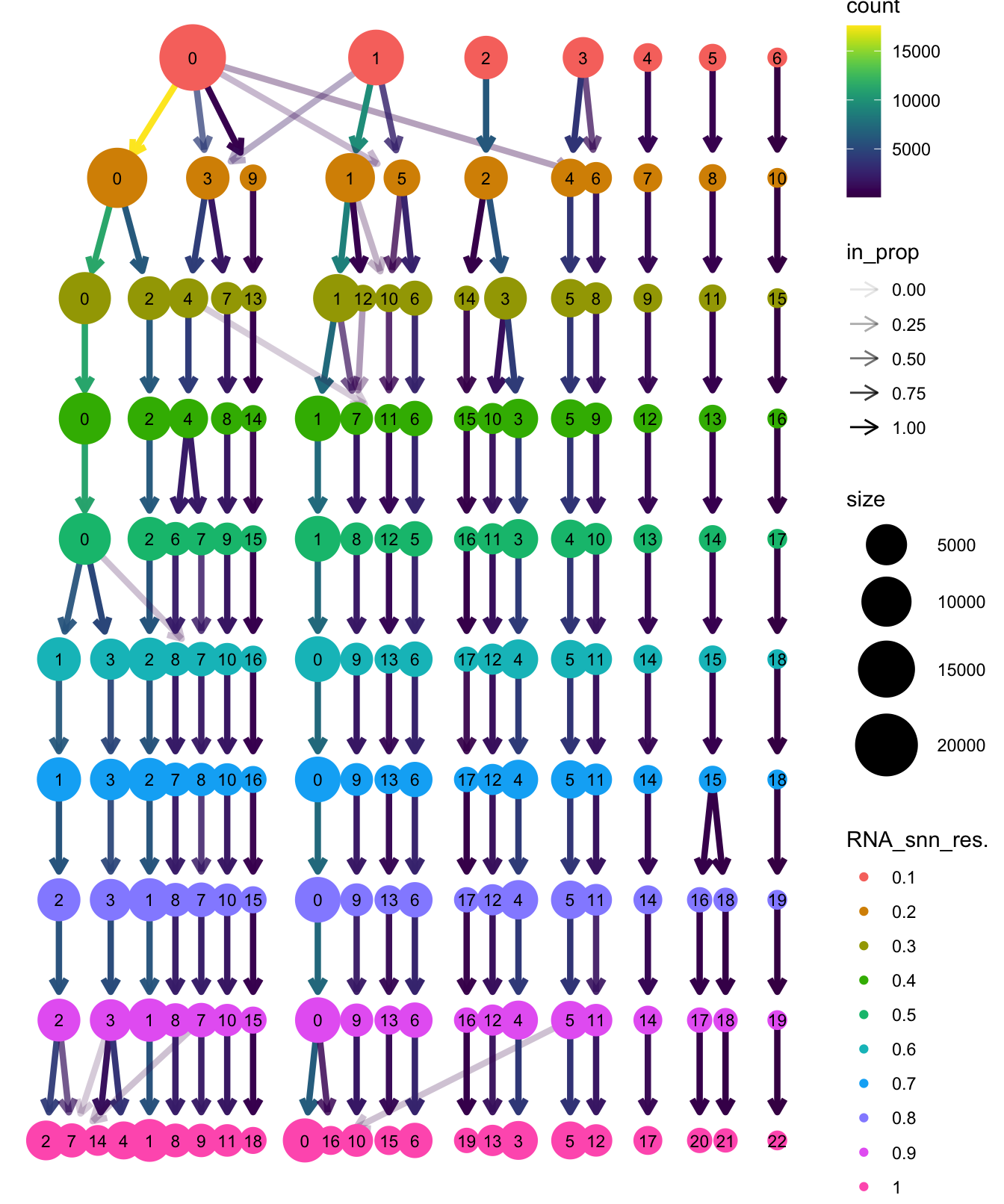
| Version | Author | Date |
|---|---|---|
| f27efbf | Gunjan Dixit | 2024-06-25 |
# Visualize the clustering results
DimPlot(paed_sub, group.by = "RNA_snn_res.0.4", reduction = "umap.new", label = TRUE, label.size = 2.5, repel = TRUE, raster = FALSE )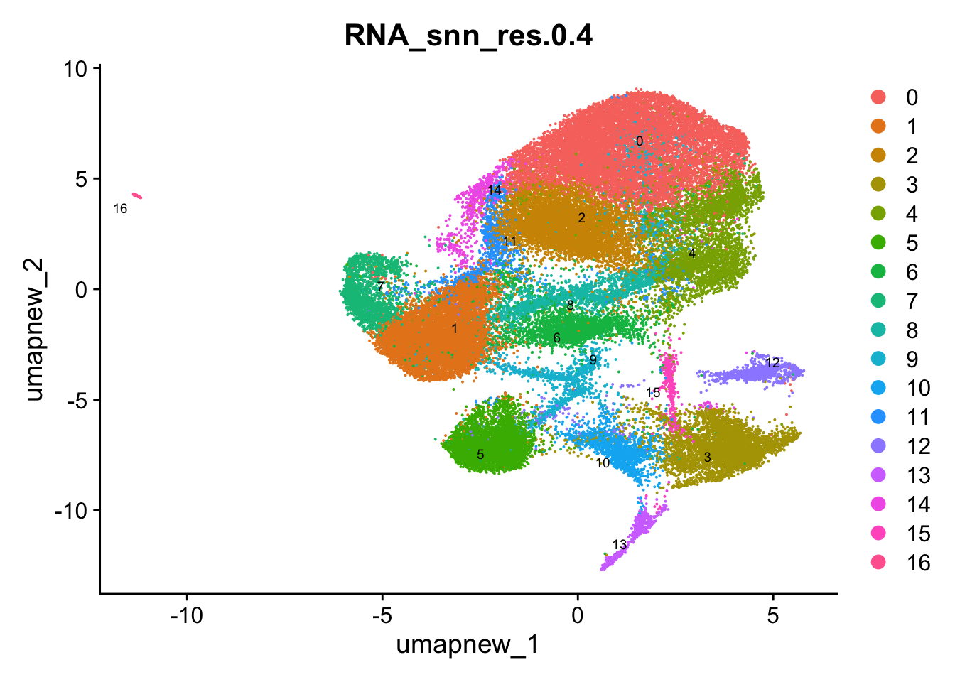
opt_res <- "RNA_snn_res.0.4"
n <- nlevels(paed_sub$RNA_snn_res.0.4)
paed_sub$RNA_snn_res.0.4 <- factor(paed_sub$RNA_snn_res.0.4, levels = seq(0,n-1))
paed_sub$seurat_clusters <- NULL
paed_sub$cluster <- paed_sub$RNA_snn_res.0.4
Idents(paed_sub) <- paed_sub$cluster
paed_sub.markers <- FindAllMarkers(paed_sub, only.pos = TRUE, min.pct = 0.25, logfc.threshold = 0.25)Calculating cluster 0Calculating cluster 1Calculating cluster 2Calculating cluster 3Calculating cluster 4Calculating cluster 5Calculating cluster 6Calculating cluster 7Calculating cluster 8Calculating cluster 9Calculating cluster 10Calculating cluster 11Calculating cluster 12Calculating cluster 13Calculating cluster 14Calculating cluster 15Calculating cluster 16paed_sub.markers %>%
group_by(cluster) %>% unique() %>%
top_n(n = 5, wt = avg_log2FC) -> top5
paed_sub.markers %>%
group_by(cluster) %>%
slice_head(n=1) %>%
pull(gene) -> best.wilcox.gene.per.cluster
best.wilcox.gene.per.cluster [1] "TOX2" "KLF2" "GPR183" "CCL5" "PRDM1" "CD8A" "KLF2" "LEF1"
[9] "FOXP3" "IFI44L" "KLRK1" "ZAP70" "GZMK" "TRDC" "ACTB" "NKG7"
[17] "DNTT" Feature plot shows the expression of top marker genes per cluster.
FeaturePlot(paed_sub,features=best.wilcox.gene.per.cluster, reduction = 'umap.new', raster = FALSE, ncol = 2, label = TRUE)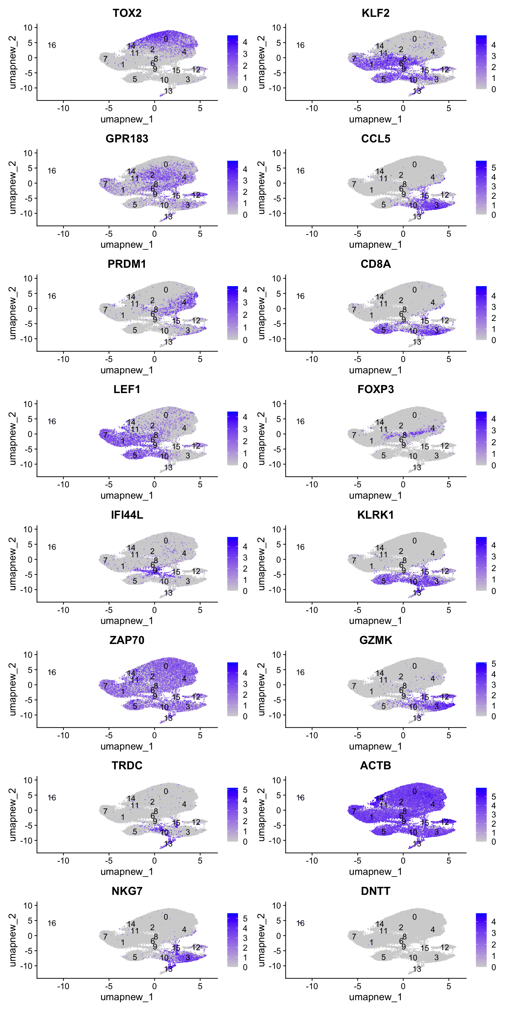
Top 10 marker genes from Seurat
## Seurat top markers
top10 <- paed_sub.markers %>%
    group_by(cluster) %>%
    top_n(n = 10, wt = avg_log2FC) %>%
    ungroup() %>%
    distinct(gene, .keep_all = TRUE) %>%
    arrange(cluster, desc(avg_log2FC))

cluster_colors <- paletteer::paletteer_d("pals::glasbey")[factor(top10$cluster)]

DotPlot(paed_sub,
        features = unique(top10$gene),
        group.by = opt_res,
        cols = c("azure1", "blueviolet"),
        dot.scale = 3, assay = "RNA") +
    RotatedAxis() +
    FontSize(y.text = 8, x.text = 12) +
    labs(y = element_blank(), x = element_blank()) +
    coord_flip() +
    theme(axis.text.y = element_text(color = cluster_colors)) +
    ggtitle("Top 10 marker genes per cluster (Seurat)")
Warning: Vectorized input to `element_text()` is not officially supported.
ℹ Results may be unexpected or may change in future versions of ggplot2.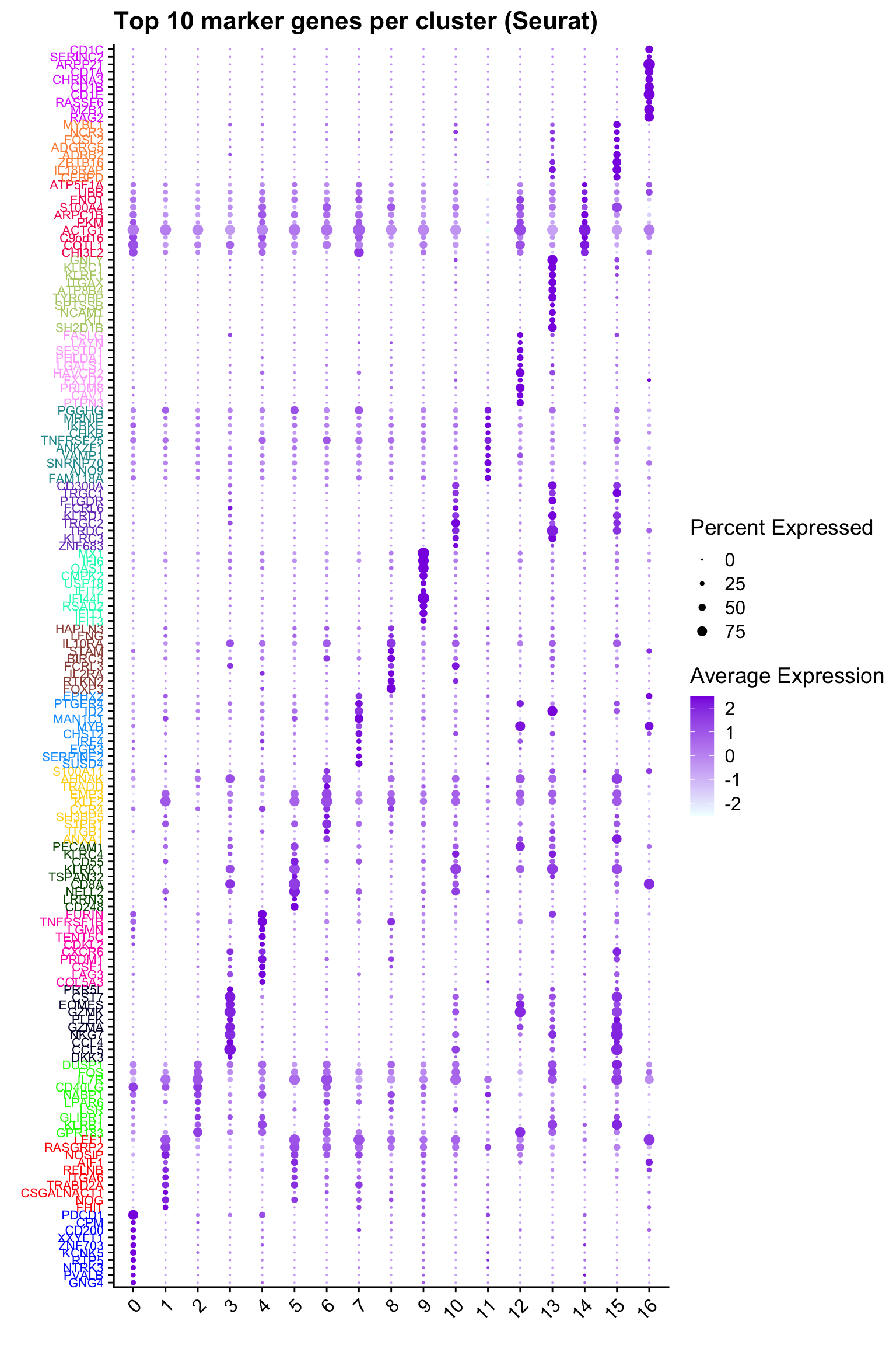
out_markers <- here("output",
            "CSV",
            paste(tissue,"_Marker_genes_Reclustered_Tcell_population.",opt_res, sep = ""))

dir.create(out_markers, recursive = TRUE, showWarnings = FALSE)

for (cl in unique(paed_sub.markers$cluster)) {
  cluster_data <- paed_sub.markers %>% dplyr::filter(cluster == cl)
  file_name <- here(out_markers, paste0("G000231_Neeland_",tissue, "_cluster_", cl, ".csv"))
  write.csv(cluster_data, file = file_name)
}
Corresponding Azimuth labels (T cell subsets)
## Level 1
DimPlot(paed_sub, reduction = "umap.new", group.by = "predicted.celltype.l1", raster = FALSE, repel = TRUE, label = TRUE, label.size = 4.5) 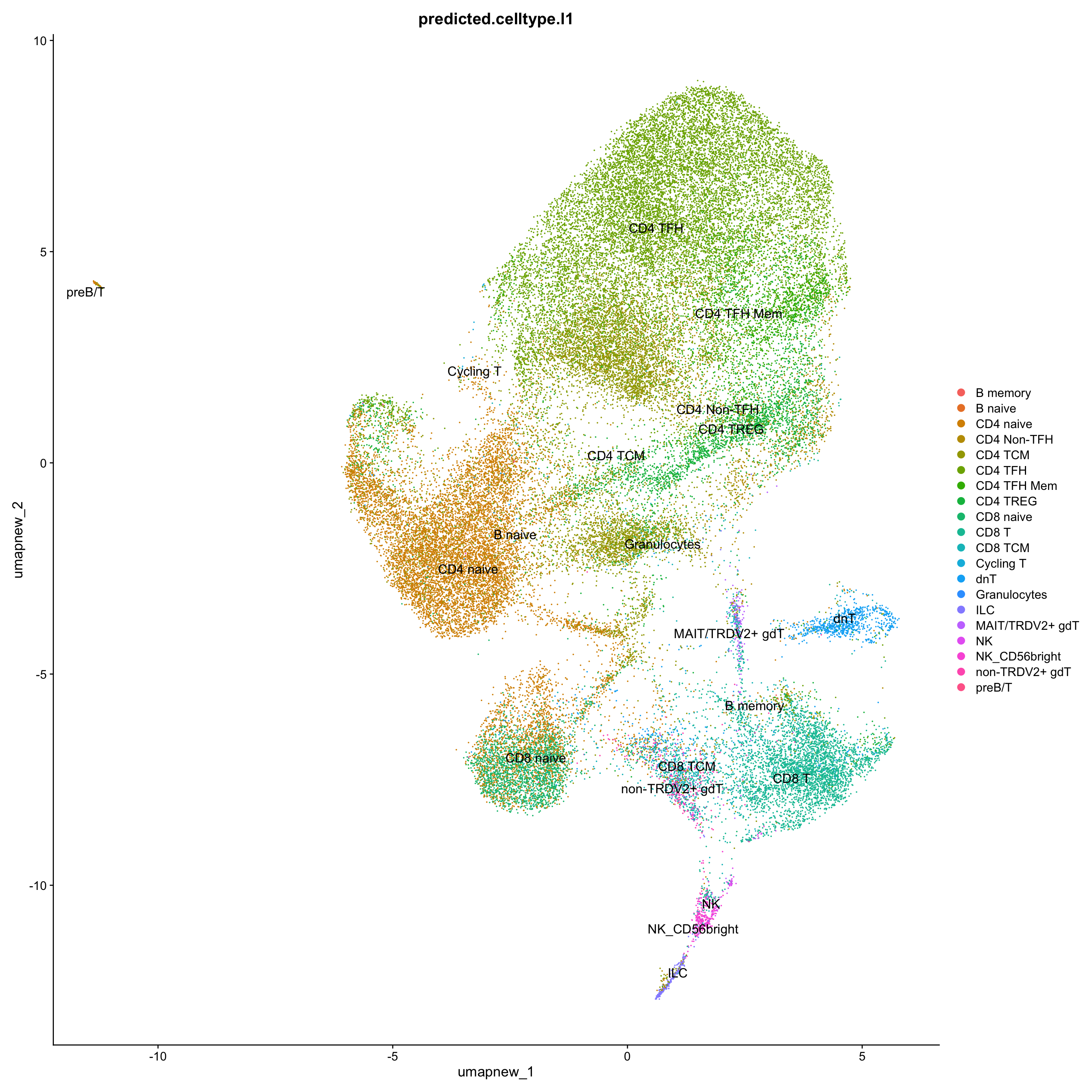
Excluding contaminating cells (B cell subtypes) for further clarity
sort(table(paed_sub$predicted.celltype.l1), decreasing = T)
        CD4 TFH       CD4 naive         CD4 TCM           CD8 T        CD4 TREG
          14687           10795            7709            3803            3352
    CD4 TFH Mem       CD8 naive     CD4 Non-TFH         CD8 TCM             dnT
           2700            2235            1574            1284            1056
 non-TRDV2+ gdT   NK_CD56bright             ILC MAIT/TRDV2+ gdT              NK
            347             260             258             156              83
      Cycling T         B naive        B memory    Granulocytes          preB/T
             22              13               4               1               1
exclude <- c("B memory", "B naive", "Granulocytes", "preB/T")
paed_sub_filtered <- paed_sub[, !paed_sub$predicted.celltype.l1 %in% exclude]
# Plots for Level 1
DimPlot(paed_sub_filtered, reduction = "umap.new", group.by = "predicted.celltype.l1", raster = FALSE, repel = TRUE, label = TRUE, label.size = 5) +
paletteer::scale_colour_paletteer_d("Polychrome::palette36")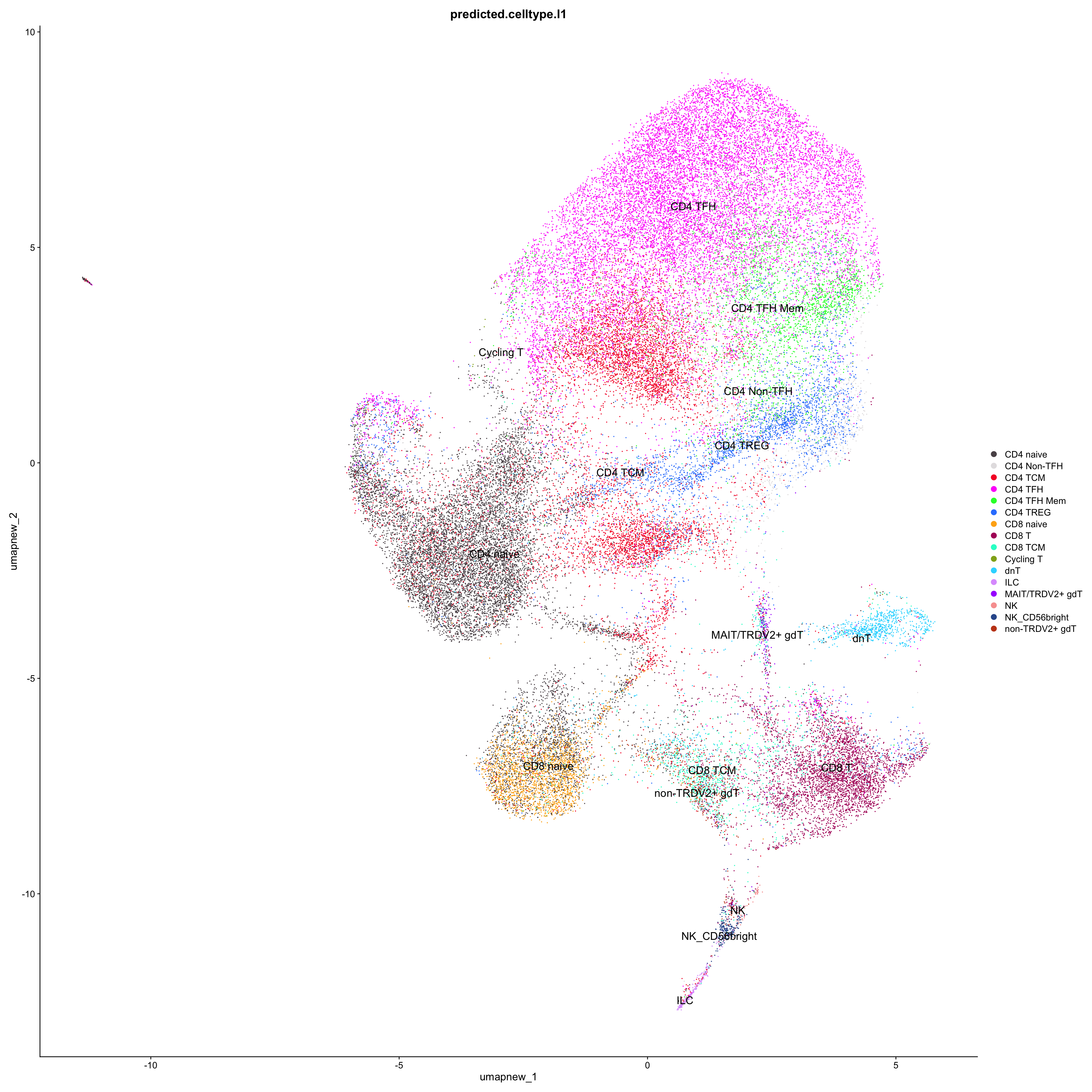
df_table_l1 <- as.data.frame(table(paed_sub_filtered$RNA_snn_res.0.4, paed_sub_filtered$predicted.celltype.l1))

ggplot(df_table_l1, aes(Var1, Freq, fill = Var2)) +
  geom_bar(stat = "identity") +
  labs(x = "RNA_snn_res.0.4", y = "Count", fill = "predicted.celltype.l1") +
  theme_minimal() +
  paletteer::scale_fill_paletteer_d("Polychrome::palette36") +
  ggtitle("Stacked Bar Plot of Tcell subsets (res=0.4) and predicted.celltype.l1")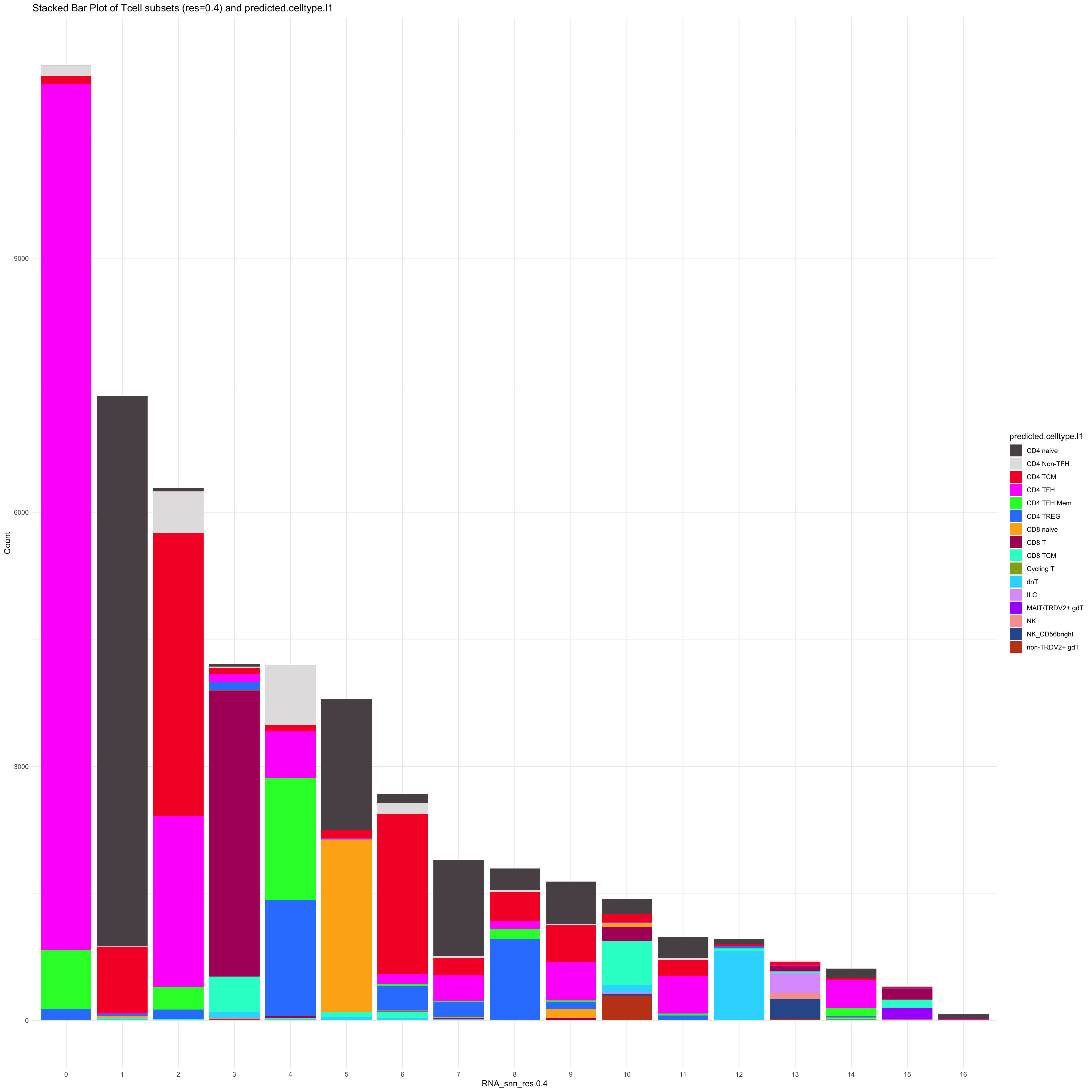
| Version | Author | Date |
|---|---|---|
| 649de68 | Gunjan Dixit | 2024-07-19 |
# Plots for Level 2
DimPlot(paed_sub_filtered, reduction = "umap.new", group.by = "predicted.celltype.l2", raster = FALSE, repel = TRUE, label = TRUE, label.size = 5)  +
    paletteer::scale_colour_paletteer_d("Polychrome::palette36")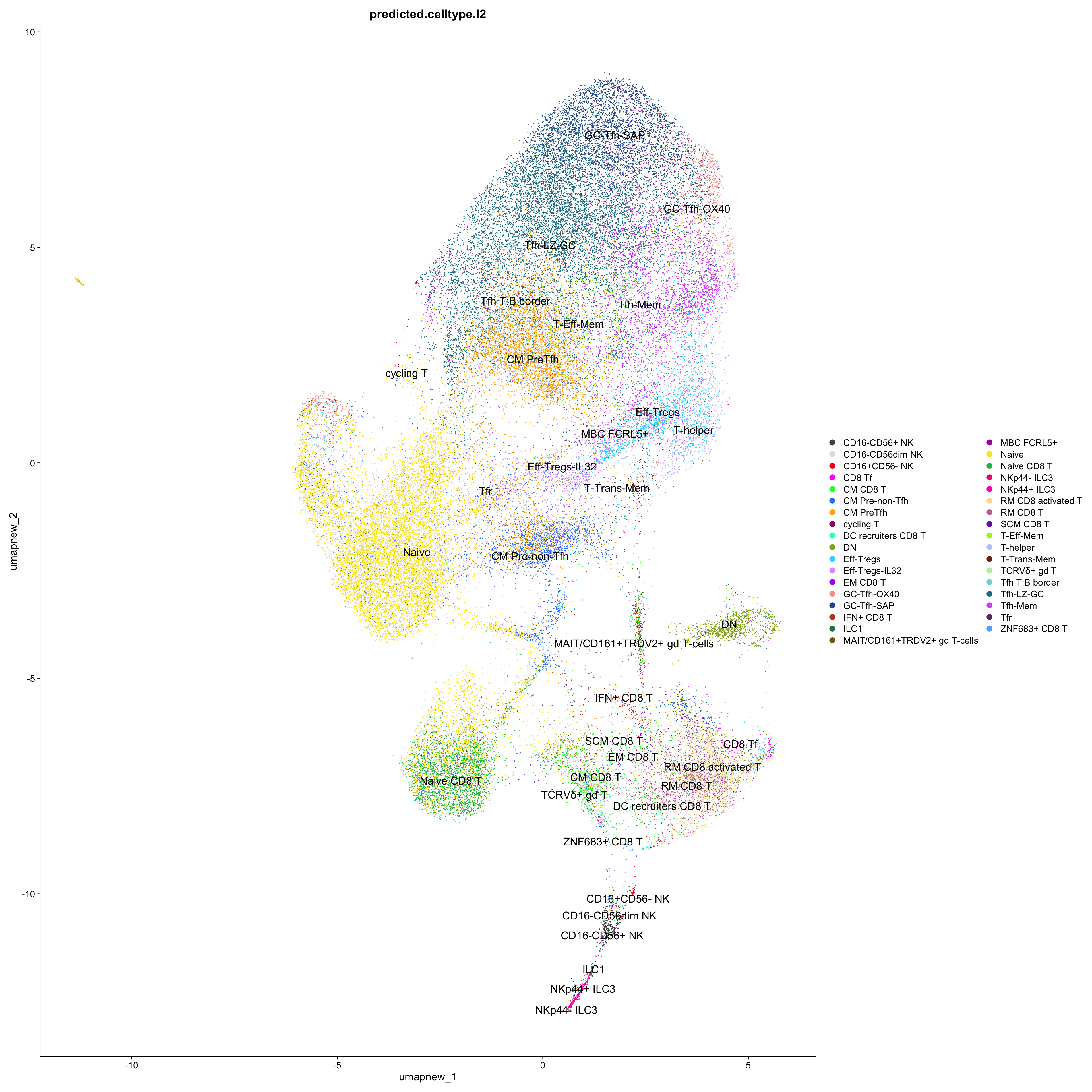
| Version | Author | Date |
|---|---|---|
| 649de68 | Gunjan Dixit | 2024-07-19 |
df_table_l2 <- as.data.frame(table(paed_sub_filtered$RNA_snn_res.0.4, paed_sub_filtered$predicted.celltype.l2))

ggplot(df_table_l2, aes(Var1, Freq, fill = Var2)) +
  geom_bar(stat = "identity") +
  labs(x = "RNA_snn_res.0.4", y = "Count", fill = "predicted.celltype.l2") +
  theme_minimal() +
  paletteer::scale_fill_paletteer_d("Polychrome::palette36") +
  ggtitle("Stacked Bar Plot of Tcell subsets (res=0.4) and predicted.celltype.l2")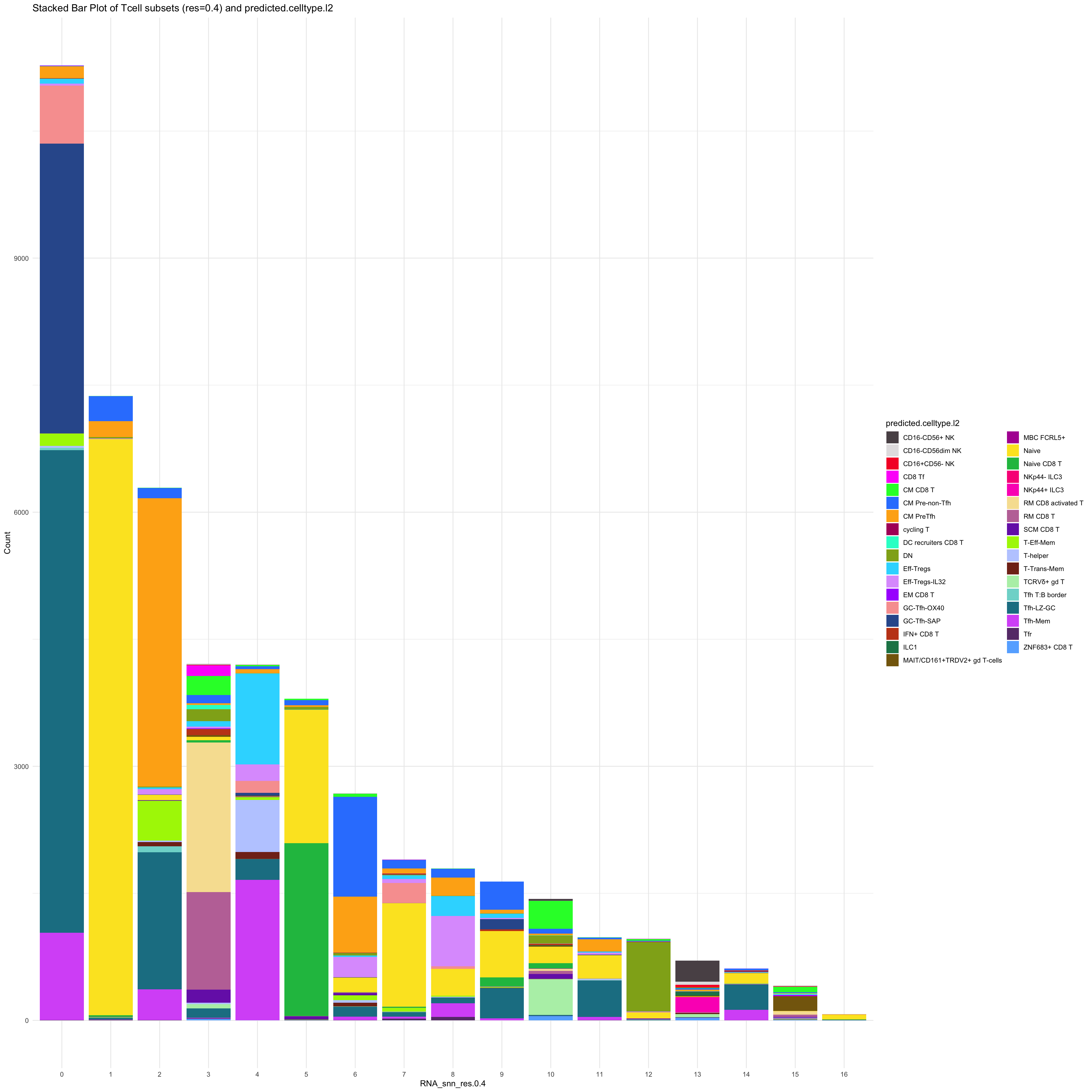
| Version | Author | Date |
|---|---|---|
| 649de68 | Gunjan Dixit | 2024-07-19 |
Reclustering GC cells
Reclustering clusters 2,5, 6, 11, 12
The marker genes for this reclustering can be found here-
sub_clusters <- c(2,5, 6, 11, 12)

idx <- which(merged_obj$cluster %in% sub_clusters)
paed_sub <- merged_obj[,idx]
paed_sub
An object of class Seurat
17566 features across 36470 samples within 1 assay
Active assay: RNA (17566 features, 2000 variable features)
3 layers present: data, counts, scale.data
4 dimensional reductions calculated: pca, umap.unintegrated, harmony, umap.harmony# Visualize the clustering results
DimPlot(paed_sub, reduction = "umap.harmony", group.by = "cluster", label = TRUE, label.size = 2.5, repel = TRUE, raster = FALSE )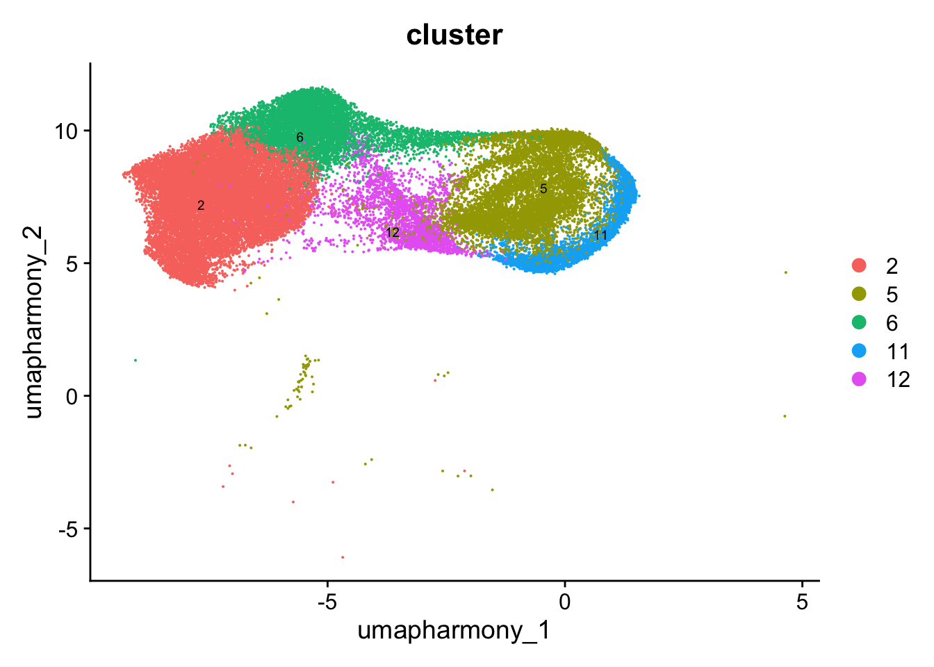
| Version | Author | Date |
|---|---|---|
| 649de68 | Gunjan Dixit | 2024-07-19 |
paed_sub <- paed_sub %>%
  NormalizeData() %>%
  FindVariableFeatures() %>%
  ScaleData() %>%
  RunPCA()

paed_sub <- RunUMAP(paed_sub, dims = 1:30, reduction = "pca", reduction.name = "umap.new")
meta_data_columns <- colnames(paed_sub@meta.data)
columns_to_remove <- grep("^RNA_snn_res", meta_data_columns, value = TRUE)
paed_sub@meta.data <- paed_sub@meta.data[, !(colnames(paed_sub@meta.data) %in% columns_to_remove)]resolutions <- seq(0.1, 1, by = 0.1)
paed_sub <- FindNeighbors(paed_sub, dims = 1:30, reduction = "pca")
paed_sub <- FindClusters(paed_sub, resolution = resolutions )Modularity Optimizer version 1.3.0 by Ludo Waltman and Nees Jan van Eck
Number of nodes: 36470
Number of edges: 1160680
Running Louvain algorithm...
Maximum modularity in 10 random starts: 0.9421
Number of communities: 4
Elapsed time: 6 seconds
Modularity Optimizer version 1.3.0 by Ludo Waltman and Nees Jan van Eck
Number of nodes: 36470
Number of edges: 1160680
Running Louvain algorithm...
Maximum modularity in 10 random starts: 0.9173
Number of communities: 8
Elapsed time: 6 seconds
Modularity Optimizer version 1.3.0 by Ludo Waltman and Nees Jan van Eck
Number of nodes: 36470
Number of edges: 1160680
Running Louvain algorithm...
Maximum modularity in 10 random starts: 0.9021
Number of communities: 11
Elapsed time: 6 seconds
Modularity Optimizer version 1.3.0 by Ludo Waltman and Nees Jan van Eck
Number of nodes: 36470
Number of edges: 1160680
Running Louvain algorithm...
Maximum modularity in 10 random starts: 0.8888
Number of communities: 13
Elapsed time: 6 seconds
Modularity Optimizer version 1.3.0 by Ludo Waltman and Nees Jan van Eck
Number of nodes: 36470
Number of edges: 1160680
Running Louvain algorithm...
Maximum modularity in 10 random starts: 0.8759
Number of communities: 15
Elapsed time: 5 seconds
Modularity Optimizer version 1.3.0 by Ludo Waltman and Nees Jan van Eck
Number of nodes: 36470
Number of edges: 1160680
Running Louvain algorithm...
Maximum modularity in 10 random starts: 0.8670
Number of communities: 15
Elapsed time: 5 seconds
Modularity Optimizer version 1.3.0 by Ludo Waltman and Nees Jan van Eck
Number of nodes: 36470
Number of edges: 1160680
Running Louvain algorithm...
Maximum modularity in 10 random starts: 0.8582
Number of communities: 17
Elapsed time: 5 seconds
Modularity Optimizer version 1.3.0 by Ludo Waltman and Nees Jan van Eck
Number of nodes: 36470
Number of edges: 1160680
Running Louvain algorithm...
Maximum modularity in 10 random starts: 0.8498
Number of communities: 18
Elapsed time: 5 seconds
Modularity Optimizer version 1.3.0 by Ludo Waltman and Nees Jan van Eck
Number of nodes: 36470
Number of edges: 1160680
Running Louvain algorithm...
Maximum modularity in 10 random starts: 0.8425
Number of communities: 19
Elapsed time: 5 seconds
Modularity Optimizer version 1.3.0 by Ludo Waltman and Nees Jan van Eck
Number of nodes: 36470
Number of edges: 1160680
Running Louvain algorithm...
Maximum modularity in 10 random starts: 0.8344
Number of communities: 20
Elapsed time: 5 secondsclustree(paed_sub, prefix = "RNA_snn_res.")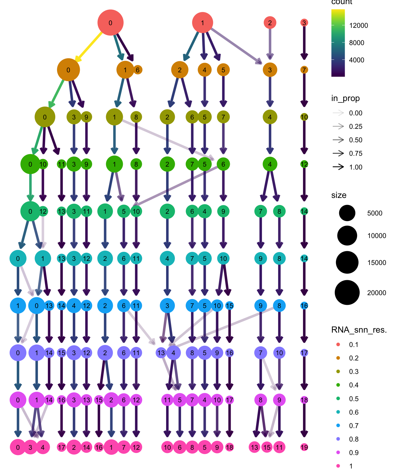
| Version | Author | Date |
|---|---|---|
| f27efbf | Gunjan Dixit | 2024-06-25 |
# Visualize the clustering results
DimPlot(paed_sub, group.by = "RNA_snn_res.0.6", reduction = "umap.new", label = TRUE, label.size = 2.5, repel = TRUE, raster = FALSE )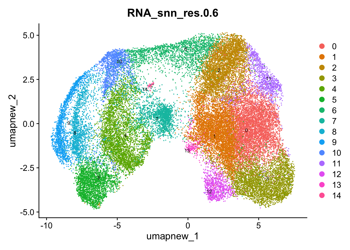
opt_res <- "RNA_snn_res.0.6"
n <- nlevels(paed_sub$RNA_snn_res.0.6)
paed_sub$RNA_snn_res.0.6 <- factor(paed_sub$RNA_snn_res.0.6, levels = seq(0,n-1))
paed_sub$seurat_clusters <- NULL
paed_sub$cluster <- paed_sub$RNA_snn_res.0.6
Idents(paed_sub) <- paed_sub$cluster
paed_sub.markers <- FindAllMarkers(paed_sub, only.pos = TRUE, min.pct = 0.25, logfc.threshold = 0.25)Calculating cluster 0Calculating cluster 1Calculating cluster 2Calculating cluster 3Calculating cluster 4Calculating cluster 5Calculating cluster 6Calculating cluster 7Calculating cluster 8Calculating cluster 9Calculating cluster 10Calculating cluster 11Calculating cluster 12Calculating cluster 13Calculating cluster 14paed_sub.markers %>%
group_by(cluster) %>% unique() %>%
top_n(n = 5, wt = avg_log2FC) -> top5
paed_sub.markers %>%
group_by(cluster) %>%
slice_head(n=1) %>%
pull(gene) -> best.wilcox.gene.per.cluster
best.wilcox.gene.per.cluster [1] "HVCN1" "LMO2" "SLC30A4" "BCL2A1" "TYMS" "MCM4"
[7] "STMN1" "TRBC2" "HIST1H2BH" "HIST1H2BB" "CDC20" "PTPRJ"
[13] "PRDM1" "XAF1" "GIMAP4" Feature plot shows the expression of top marker genes per cluster.
FeaturePlot(paed_sub,features=best.wilcox.gene.per.cluster, reduction = 'umap.new', raster = FALSE, ncol = 2, label = TRUE)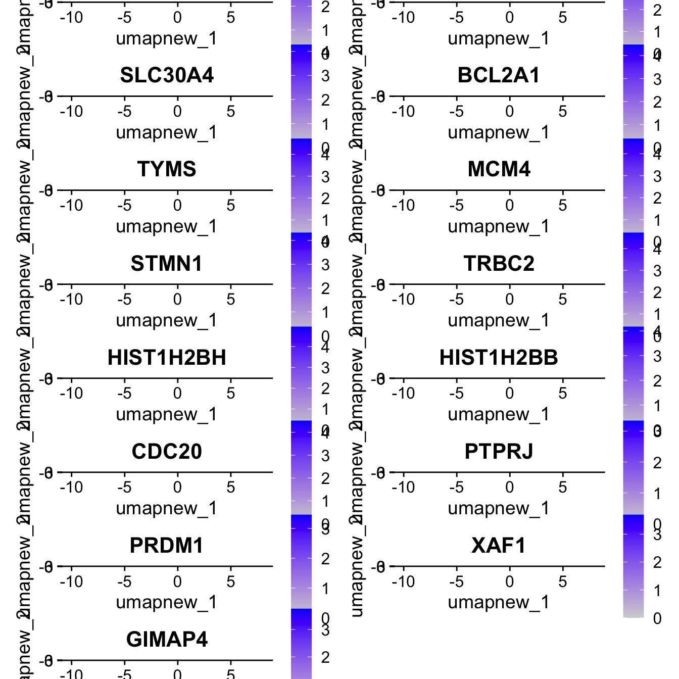
Top 10 marker genes from Seurat
## Seurat top markers
top10 <- paed_sub.markers %>%
    group_by(cluster) %>%
    top_n(n = 10, wt = avg_log2FC) %>%
    ungroup() %>%
    distinct(gene, .keep_all = TRUE) %>%
    arrange(cluster, desc(avg_log2FC))

cluster_colors <- paletteer::paletteer_d("pals::glasbey")[factor(top10$cluster)]

DotPlot(paed_sub,
        features = unique(top10$gene),
        group.by = opt_res,
        cols = c("azure1", "blueviolet"),
        dot.scale = 3, assay = "RNA") +
    RotatedAxis() +
    FontSize(y.text = 8, x.text = 12) +
    labs(y = element_blank(), x = element_blank()) +
    coord_flip() +
    theme(axis.text.y = element_text(color = cluster_colors)) +
    ggtitle("Top 10 marker genes per cluster (Seurat)")
Warning: Vectorized input to `element_text()` is not officially supported.
ℹ Results may be unexpected or may change in future versions of ggplot2.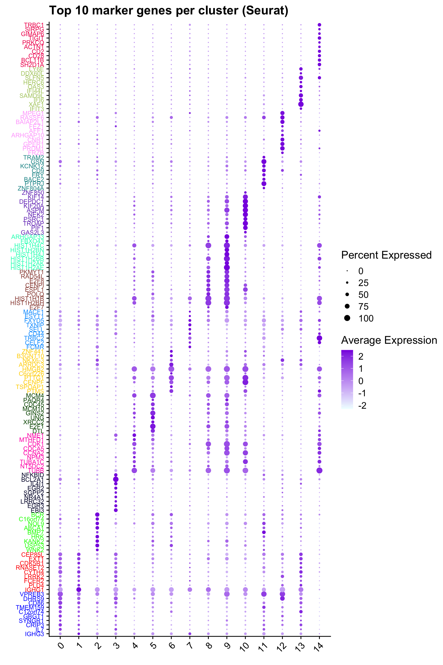
| Version | Author | Date |
|---|---|---|
| 649de68 | Gunjan Dixit | 2024-07-19 |
out_markers <- here("output",
            "CSV",
            paste(tissue,"_Marker_genes_Reclustered_GC_population.",opt_res, sep = ""))

dir.create(out_markers, recursive = TRUE, showWarnings = FALSE)

for (cl in unique(paed_sub.markers$cluster)) {
  cluster_data <- paed_sub.markers %>% dplyr::filter(cluster == cl)
  file_name <- here(out_markers, paste0("G000231_Neeland_",tissue, "_cluster_", cl, ".csv"))
  write.csv(cluster_data, file = file_name)
}
Corresponding Azimuth labels (GC cell subsets)
## Level 1
DimPlot(paed_sub, reduction = "umap.new", group.by = "predicted.celltype.l1", raster = FALSE, repel = TRUE, label = TRUE, label.size = 4.5) 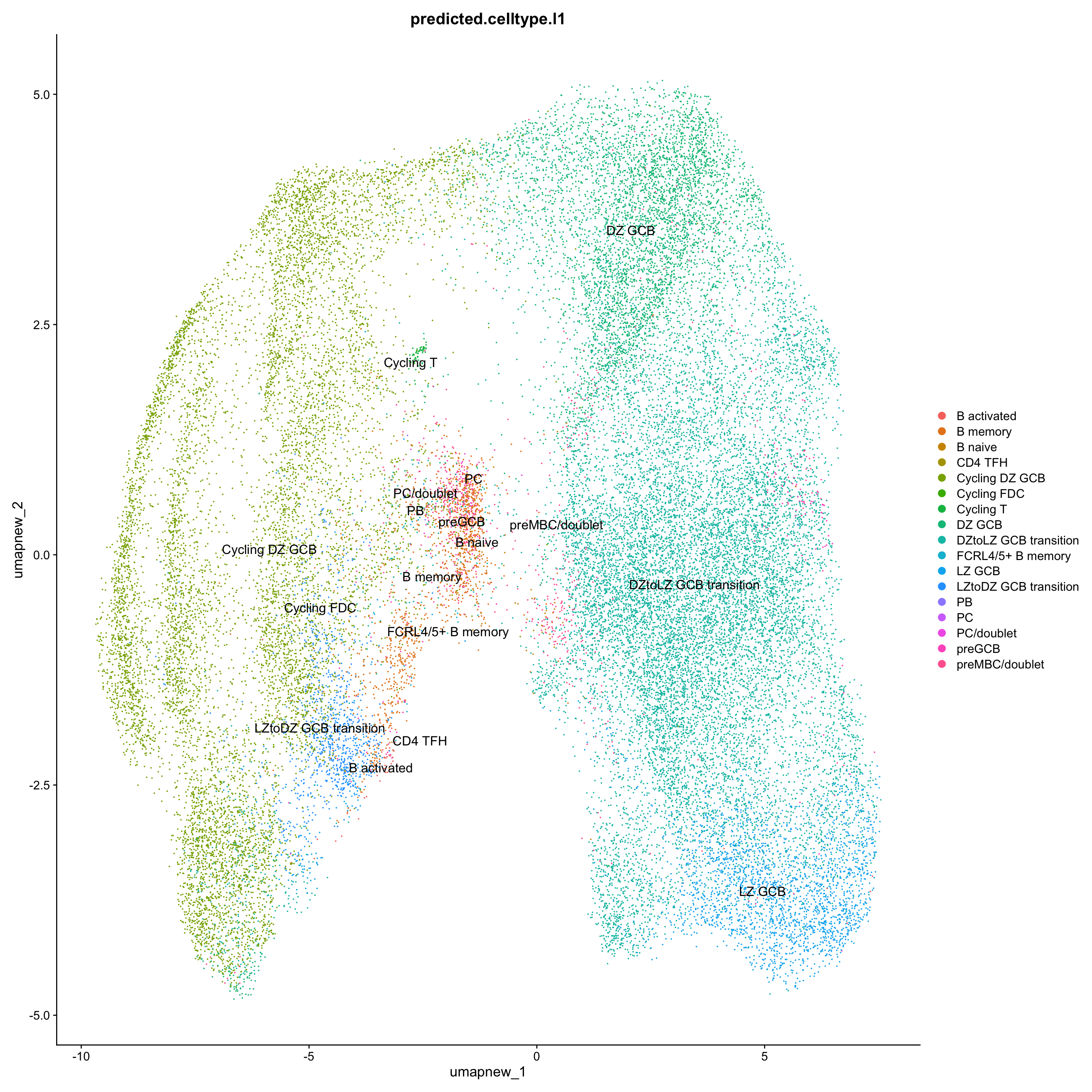
| Version | Author | Date |
|---|---|---|
| 649de68 | Gunjan Dixit | 2024-07-19 |
df_table <- as.data.frame(table(paed_sub$RNA_snn_res.0.6, paed_sub$predicted.celltype.l1))
ggplot(df_table, aes(Var1, Freq, fill = Var2)) +
  geom_bar(stat = "identity") +
  labs(x = "RNA_snn_res.0.6", y = "Count", fill = "predicted.celltype.l1") +
  theme_minimal() +
  ggtitle("Stacked Bar Plot of Tcell subsets (res=0.6) and predicted.celltype.l1")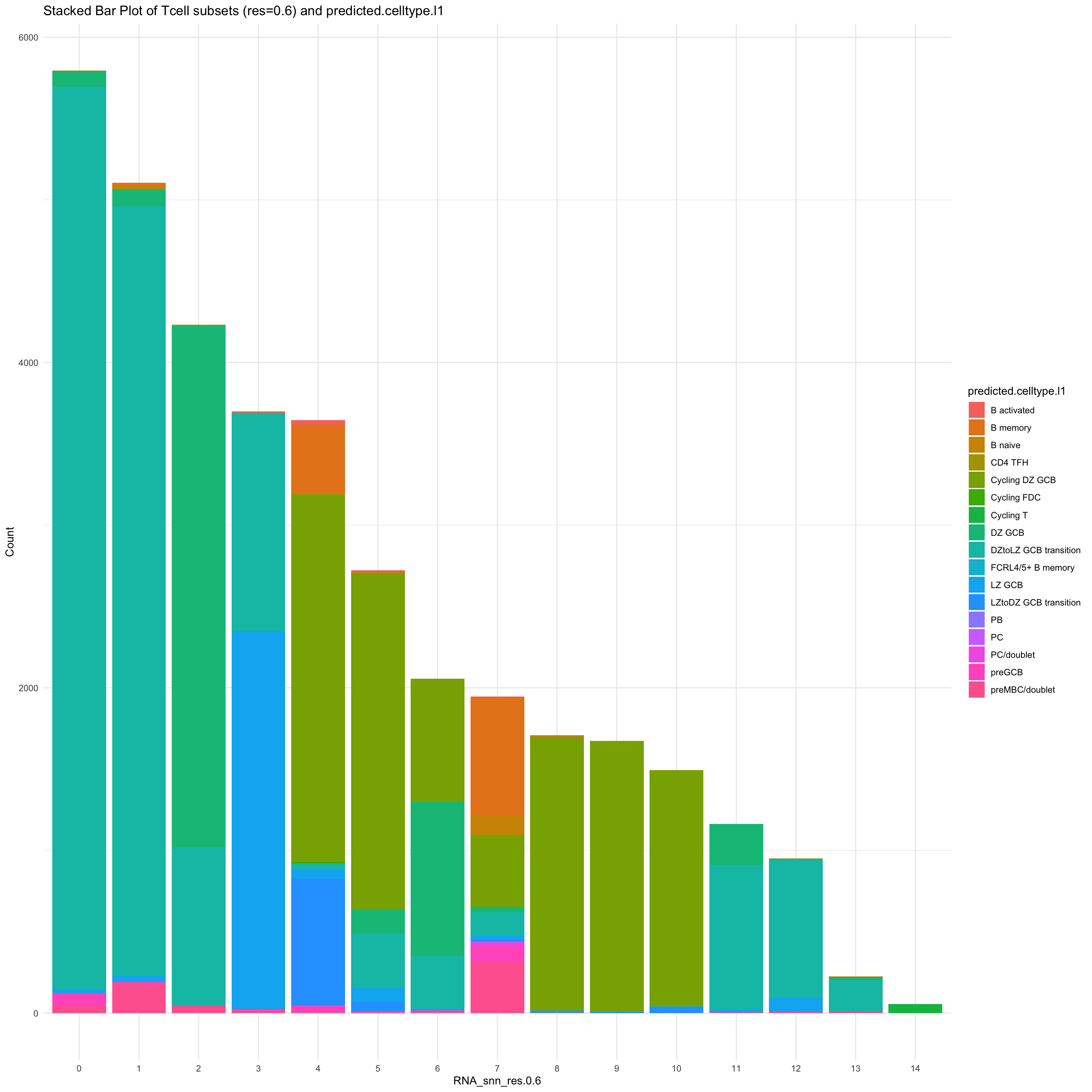
| Version | Author | Date |
|---|---|---|
| 649de68 | Gunjan Dixit | 2024-07-19 |
Confirm cluster 13 (activated DC3)
From Mel’s notes: Confirming CCR7 and LAMP3 expression in cluster 13 currently labelled as “activated DC3 (aDC3)?”
idx <- which(merged_obj$cluster %in% 13)
paed_sub <- merged_obj[,idx]
paed_sub
An object of class Seurat
17566 features across 2349 samples within 1 assay
Active assay: RNA (17566 features, 2000 variable features)
3 layers present: data, counts, scale.data
4 dimensional reductions calculated: pca, umap.unintegrated, harmony, umap.harmonyFeaturePlot(paed_sub,features=c("CCR7","LAMP3"), reduction = 'umap.harmony', ncol = 1, label = FALSE)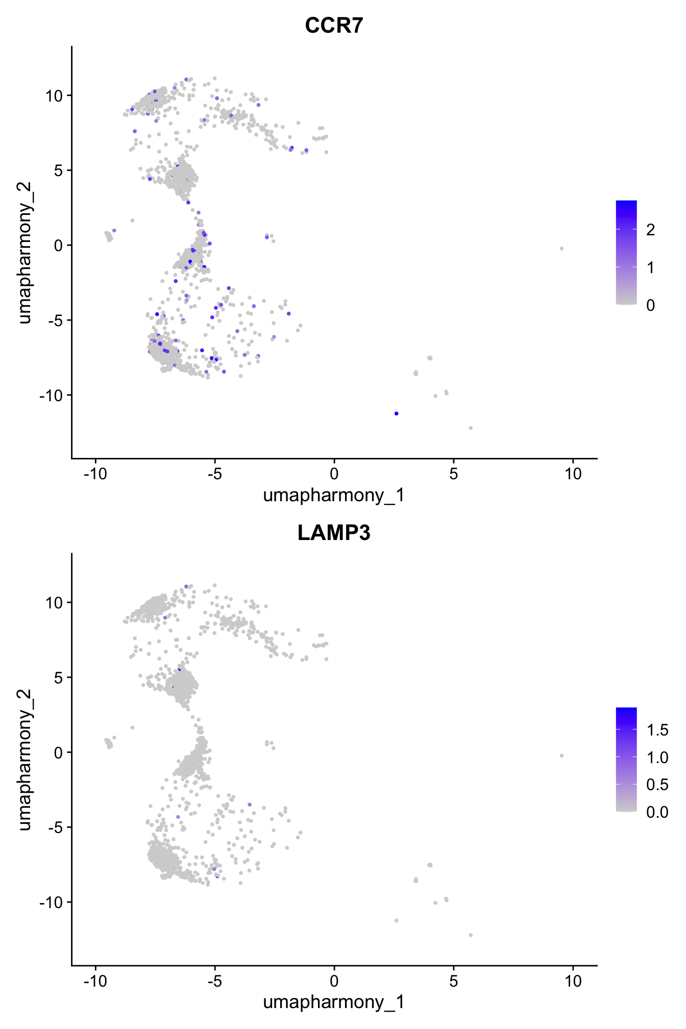
| Version | Author | Date |
|---|---|---|
| 649de68 | Gunjan Dixit | 2024-07-19 |
Session Info
sessioninfo::session_info()─ Session info ───────────────────────────────────────────────────────────────
setting value
version R version 4.3.2 (2023-10-31)
os macOS Sonoma 14.5
system aarch64, darwin20
ui X11
language (EN)
collate en_US.UTF-8
ctype en_US.UTF-8
tz Australia/Melbourne
date 2024-07-26
pandoc 3.1.1 @ /Users/dixitgunjan/Desktop/RStudio.app/Contents/Resources/app/quarto/bin/tools/ (via rmarkdown)
─ Packages ───────────────────────────────────────────────────────────────────
package * version date (UTC) lib source
abind 1.4-5 2016-07-21 [1] CRAN (R 4.3.0)
backports 1.4.1 2021-12-13 [1] CRAN (R 4.3.0)
beeswarm 0.4.0 2021-06-01 [1] CRAN (R 4.3.0)
BiocManager 1.30.22 2023-08-08 [1] CRAN (R 4.3.0)
BiocStyle * 2.30.0 2023-10-26 [1] Bioconductor
bslib 0.6.1 2023-11-28 [1] CRAN (R 4.3.1)
cachem 1.0.8 2023-05-01 [1] CRAN (R 4.3.0)
callr 3.7.5 2024-02-19 [1] CRAN (R 4.3.1)
cellranger 1.1.0 2016-07-27 [1] CRAN (R 4.3.0)
checkmate 2.3.1 2023-12-04 [1] CRAN (R 4.3.1)
cli 3.6.2 2023-12-11 [1] CRAN (R 4.3.1)
cluster 2.1.6 2023-12-01 [1] CRAN (R 4.3.1)
clustree * 0.5.1 2023-11-05 [1] CRAN (R 4.3.1)
codetools 0.2-19 2023-02-01 [1] CRAN (R 4.3.2)
colorspace 2.1-0 2023-01-23 [1] CRAN (R 4.3.0)
cowplot 1.1.3 2024-01-22 [1] CRAN (R 4.3.1)
data.table * 1.15.0 2024-01-30 [1] CRAN (R 4.3.1)
deldir 2.0-2 2023-11-23 [1] CRAN (R 4.3.1)
digest 0.6.34 2024-01-11 [1] CRAN (R 4.3.1)
dotCall64 1.1-1 2023-11-28 [1] CRAN (R 4.3.1)
dplyr * 1.1.4 2023-11-17 [1] CRAN (R 4.3.1)
ellipsis 0.3.2 2021-04-29 [1] CRAN (R 4.3.0)
evaluate 0.23 2023-11-01 [1] CRAN (R 4.3.1)
fansi 1.0.6 2023-12-08 [1] CRAN (R 4.3.1)
farver 2.1.1 2022-07-06 [1] CRAN (R 4.3.0)
fastDummies 1.7.3 2023-07-06 [1] CRAN (R 4.3.0)
fastmap 1.1.1 2023-02-24 [1] CRAN (R 4.3.0)
fitdistrplus 1.1-11 2023-04-25 [1] CRAN (R 4.3.0)
forcats * 1.0.0 2023-01-29 [1] CRAN (R 4.3.0)
fs 1.6.3 2023-07-20 [1] CRAN (R 4.3.0)
future 1.33.1 2023-12-22 [1] CRAN (R 4.3.1)
future.apply 1.11.1 2023-12-21 [1] CRAN (R 4.3.1)
generics 0.1.3 2022-07-05 [1] CRAN (R 4.3.0)
getPass 0.2-4 2023-12-10 [1] CRAN (R 4.3.1)
ggbeeswarm 0.7.2 2023-04-29 [1] CRAN (R 4.3.0)
ggforce 0.4.2 2024-02-19 [1] CRAN (R 4.3.1)
ggplot2 * 3.5.0 2024-02-23 [1] CRAN (R 4.3.1)
ggraph * 2.1.0 2022-10-09 [1] CRAN (R 4.3.0)
ggrastr 1.0.2 2023-06-01 [1] CRAN (R 4.3.0)
ggrepel 0.9.5 2024-01-10 [1] CRAN (R 4.3.1)
ggridges 0.5.6 2024-01-23 [1] CRAN (R 4.3.1)
git2r 0.33.0 2023-11-26 [1] CRAN (R 4.3.1)
globals 0.16.2 2022-11-21 [1] CRAN (R 4.3.0)
glue 1.7.0 2024-01-09 [1] CRAN (R 4.3.1)
goftest 1.2-3 2021-10-07 [1] CRAN (R 4.3.0)
graphlayouts 1.1.0 2024-01-19 [1] CRAN (R 4.3.1)
gridExtra 2.3 2017-09-09 [1] CRAN (R 4.3.0)
gtable 0.3.4 2023-08-21 [1] CRAN (R 4.3.0)
here * 1.0.1 2020-12-13 [1] CRAN (R 4.3.0)
highr 0.10 2022-12-22 [1] CRAN (R 4.3.0)
hms 1.1.3 2023-03-21 [1] CRAN (R 4.3.0)
htmltools 0.5.7 2023-11-03 [1] CRAN (R 4.3.1)
htmlwidgets 1.6.4 2023-12-06 [1] CRAN (R 4.3.1)
httpuv 1.6.14 2024-01-26 [1] CRAN (R 4.3.1)
httr 1.4.7 2023-08-15 [1] CRAN (R 4.3.0)
ica 1.0-3 2022-07-08 [1] CRAN (R 4.3.0)
igraph 2.0.2 2024-02-17 [1] CRAN (R 4.3.1)
irlba 2.3.5.1 2022-10-03 [1] CRAN (R 4.3.2)
jquerylib 0.1.4 2021-04-26 [1] CRAN (R 4.3.0)
jsonlite 1.8.8 2023-12-04 [1] CRAN (R 4.3.1)
kableExtra * 1.4.0 2024-01-24 [1] CRAN (R 4.3.1)
KernSmooth 2.23-22 2023-07-10 [1] CRAN (R 4.3.2)
knitr 1.45 2023-10-30 [1] CRAN (R 4.3.1)
labeling 0.4.3 2023-08-29 [1] CRAN (R 4.3.0)
later 1.3.2 2023-12-06 [1] CRAN (R 4.3.1)
lattice 0.22-5 2023-10-24 [1] CRAN (R 4.3.1)
lazyeval 0.2.2 2019-03-15 [1] CRAN (R 4.3.0)
leiden 0.4.3.1 2023-11-17 [1] CRAN (R 4.3.1)
lifecycle 1.0.4 2023-11-07 [1] CRAN (R 4.3.1)
limma 3.58.1 2023-11-02 [1] Bioconductor
listenv 0.9.1 2024-01-29 [1] CRAN (R 4.3.1)
lmtest 0.9-40 2022-03-21 [1] CRAN (R 4.3.0)
lubridate * 1.9.3 2023-09-27 [1] CRAN (R 4.3.1)
magrittr 2.0.3 2022-03-30 [1] CRAN (R 4.3.0)
MASS 7.3-60.0.1 2024-01-13 [1] CRAN (R 4.3.1)
Matrix 1.6-5 2024-01-11 [1] CRAN (R 4.3.1)
matrixStats 1.2.0 2023-12-11 [1] CRAN (R 4.3.1)
mime 0.12 2021-09-28 [1] CRAN (R 4.3.0)
miniUI 0.1.1.1 2018-05-18 [1] CRAN (R 4.3.0)
munsell 0.5.0 2018-06-12 [1] CRAN (R 4.3.0)
nlme 3.1-164 2023-11-27 [1] CRAN (R 4.3.1)
paletteer 1.6.0 2024-01-21 [1] CRAN (R 4.3.1)
parallelly 1.37.0 2024-02-14 [1] CRAN (R 4.3.1)
patchwork * 1.2.0 2024-01-08 [1] CRAN (R 4.3.1)
pbapply 1.7-2 2023-06-27 [1] CRAN (R 4.3.0)
pillar 1.9.0 2023-03-22 [1] CRAN (R 4.3.0)
pkgconfig 2.0.3 2019-09-22 [1] CRAN (R 4.3.0)
plotly 4.10.4 2024-01-13 [1] CRAN (R 4.3.1)
plyr 1.8.9 2023-10-02 [1] CRAN (R 4.3.1)
png 0.1-8 2022-11-29 [1] CRAN (R 4.3.0)
polyclip 1.10-6 2023-09-27 [1] CRAN (R 4.3.1)
presto 1.0.0 2024-02-27 [1] Github (immunogenomics/presto@31dc97f)
prismatic 1.1.1 2022-08-15 [1] CRAN (R 4.3.0)
processx 3.8.3 2023-12-10 [1] CRAN (R 4.3.1)
progressr 0.14.0 2023-08-10 [1] CRAN (R 4.3.0)
promises 1.2.1 2023-08-10 [1] CRAN (R 4.3.0)
ps 1.7.6 2024-01-18 [1] CRAN (R 4.3.1)
purrr * 1.0.2 2023-08-10 [1] CRAN (R 4.3.0)
R6 2.5.1 2021-08-19 [1] CRAN (R 4.3.0)
RANN 2.6.1 2019-01-08 [1] CRAN (R 4.3.0)
RColorBrewer * 1.1-3 2022-04-03 [1] CRAN (R 4.3.0)
Rcpp 1.0.12 2024-01-09 [1] CRAN (R 4.3.1)
RcppAnnoy 0.0.22 2024-01-23 [1] CRAN (R 4.3.1)
RcppHNSW 0.6.0 2024-02-04 [1] CRAN (R 4.3.1)
readr * 2.1.5 2024-01-10 [1] CRAN (R 4.3.1)
readxl 1.4.3 2023-07-06 [1] CRAN (R 4.3.0)
rematch2 2.1.2 2020-05-01 [1] CRAN (R 4.3.0)
reshape2 1.4.4 2020-04-09 [1] CRAN (R 4.3.0)
reticulate 1.35.0 2024-01-31 [1] CRAN (R 4.3.1)
rlang 1.1.3 2024-01-10 [1] CRAN (R 4.3.1)
rmarkdown 2.25 2023-09-18 [1] CRAN (R 4.3.1)
ROCR 1.0-11 2020-05-02 [1] CRAN (R 4.3.0)
rprojroot 2.0.4 2023-11-05 [1] CRAN (R 4.3.1)
RSpectra 0.16-1 2022-04-24 [1] CRAN (R 4.3.0)
rstudioapi 0.15.0 2023-07-07 [1] CRAN (R 4.3.0)
Rtsne 0.17 2023-12-07 [1] CRAN (R 4.3.1)
sass 0.4.8 2023-12-06 [1] CRAN (R 4.3.1)
scales 1.3.0 2023-11-28 [1] CRAN (R 4.3.1)
scattermore 1.2 2023-06-12 [1] CRAN (R 4.3.0)
sctransform 0.4.1 2023-10-19 [1] CRAN (R 4.3.1)
sessioninfo 1.2.2 2021-12-06 [1] CRAN (R 4.3.0)
Seurat * 5.0.1.9009 2024-02-28 [1] Github (satijalab/seurat@6a3ef5e)
SeuratObject * 5.0.1 2023-11-17 [1] CRAN (R 4.3.1)
shiny 1.8.0 2023-11-17 [1] CRAN (R 4.3.1)
sp * 2.1-3 2024-01-30 [1] CRAN (R 4.3.1)
spam 2.10-0 2023-10-23 [1] CRAN (R 4.3.1)
spatstat.data 3.0-4 2024-01-15 [1] CRAN (R 4.3.1)
spatstat.explore 3.2-6 2024-02-01 [1] CRAN (R 4.3.1)
spatstat.geom 3.2-8 2024-01-26 [1] CRAN (R 4.3.1)
spatstat.random 3.2-2 2023-11-29 [1] CRAN (R 4.3.1)
spatstat.sparse 3.0-3 2023-10-24 [1] CRAN (R 4.3.1)
spatstat.utils 3.0-4 2023-10-24 [1] CRAN (R 4.3.1)
statmod 1.5.0 2023-01-06 [1] CRAN (R 4.3.0)
stringi 1.8.3 2023-12-11 [1] CRAN (R 4.3.1)
stringr * 1.5.1 2023-11-14 [1] CRAN (R 4.3.1)
survival 3.5-8 2024-02-14 [1] CRAN (R 4.3.1)
svglite 2.1.3 2023-12-08 [1] CRAN (R 4.3.1)
systemfonts 1.0.5 2023-10-09 [1] CRAN (R 4.3.1)
tensor 1.5 2012-05-05 [1] CRAN (R 4.3.0)
tibble * 3.2.1 2023-03-20 [1] CRAN (R 4.3.0)
tidygraph 1.3.1 2024-01-30 [1] CRAN (R 4.3.1)
tidyr * 1.3.1 2024-01-24 [1] CRAN (R 4.3.1)
tidyselect 1.2.0 2022-10-10 [1] CRAN (R 4.3.0)
tidyverse * 2.0.0 2023-02-22 [1] CRAN (R 4.3.0)
timechange 0.3.0 2024-01-18 [1] CRAN (R 4.3.1)
tweenr 2.0.3 2024-02-26 [1] CRAN (R 4.3.1)
tzdb 0.4.0 2023-05-12 [1] CRAN (R 4.3.0)
utf8 1.2.4 2023-10-22 [1] CRAN (R 4.3.1)
uwot 0.1.16 2023-06-29 [1] CRAN (R 4.3.0)
vctrs 0.6.5 2023-12-01 [1] CRAN (R 4.3.1)
vipor 0.4.7 2023-12-18 [1] CRAN (R 4.3.1)
viridis 0.6.5 2024-01-29 [1] CRAN (R 4.3.1)
viridisLite 0.4.2 2023-05-02 [1] CRAN (R 4.3.0)
whisker 0.4.1 2022-12-05 [1] CRAN (R 4.3.0)
withr 3.0.0 2024-01-16 [1] CRAN (R 4.3.1)
workflowr * 1.7.1 2023-08-23 [1] CRAN (R 4.3.0)
xfun 0.42 2024-02-08 [1] CRAN (R 4.3.1)
xml2 1.3.6 2023-12-04 [1] CRAN (R 4.3.1)
xtable 1.8-4 2019-04-21 [1] CRAN (R 4.3.0)
yaml 2.3.8 2023-12-11 [1] CRAN (R 4.3.1)
zoo 1.8-12 2023-04-13 [1] CRAN (R 4.3.0)
[1] /Library/Frameworks/R.framework/Versions/4.3-arm64/Resources/library
──────────────────────────────────────────────────────────────────────────────
sessionInfo()R version 4.3.2 (2023-10-31)
Platform: aarch64-apple-darwin20 (64-bit)
Running under: macOS Sonoma 14.5
Matrix products: default
BLAS: /Library/Frameworks/R.framework/Versions/4.3-arm64/Resources/lib/libRblas.0.dylib
LAPACK: /Library/Frameworks/R.framework/Versions/4.3-arm64/Resources/lib/libRlapack.dylib; LAPACK version 3.11.0
locale:
[1] en_US.UTF-8/en_US.UTF-8/en_US.UTF-8/C/en_US.UTF-8/en_US.UTF-8
time zone: Australia/Melbourne
tzcode source: internal
attached base packages:
[1] stats graphics grDevices utils datasets methods base
other attached packages:
[1] patchwork_1.2.0 data.table_1.15.0 RColorBrewer_1.1-3 kableExtra_1.4.0
[5] clustree_0.5.1 ggraph_2.1.0 Seurat_5.0.1.9009 SeuratObject_5.0.1
[9] sp_2.1-3 here_1.0.1 lubridate_1.9.3 forcats_1.0.0
[13] stringr_1.5.1 dplyr_1.1.4 purrr_1.0.2 readr_2.1.5
[17] tidyr_1.3.1 tibble_3.2.1 ggplot2_3.5.0 tidyverse_2.0.0
[21] BiocStyle_2.30.0 workflowr_1.7.1
loaded via a namespace (and not attached):
[1] RcppAnnoy_0.0.22 splines_4.3.2 later_1.3.2
[4] prismatic_1.1.1 cellranger_1.1.0 polyclip_1.10-6
[7] fastDummies_1.7.3 lifecycle_1.0.4 rprojroot_2.0.4
[10] globals_0.16.2 processx_3.8.3 lattice_0.22-5
[13] MASS_7.3-60.0.1 backports_1.4.1 magrittr_2.0.3
[16] limma_3.58.1 plotly_4.10.4 sass_0.4.8
[19] rmarkdown_2.25 jquerylib_0.1.4 yaml_2.3.8
[22] httpuv_1.6.14 sctransform_0.4.1 spam_2.10-0
[25] sessioninfo_1.2.2 spatstat.sparse_3.0-3 reticulate_1.35.0
[28] cowplot_1.1.3 pbapply_1.7-2 abind_1.4-5
[31] Rtsne_0.17 presto_1.0.0 tweenr_2.0.3
[34] git2r_0.33.0 ggrepel_0.9.5 irlba_2.3.5.1
[37] listenv_0.9.1 spatstat.utils_3.0-4 goftest_1.2-3
[40] RSpectra_0.16-1 spatstat.random_3.2-2 fitdistrplus_1.1-11
[43] parallelly_1.37.0 svglite_2.1.3 leiden_0.4.3.1
[46] codetools_0.2-19 xml2_1.3.6 ggforce_0.4.2
[49] tidyselect_1.2.0 farver_2.1.1 viridis_0.6.5
[52] matrixStats_1.2.0 spatstat.explore_3.2-6 jsonlite_1.8.8
[55] ellipsis_0.3.2 tidygraph_1.3.1 progressr_0.14.0
[58] ggridges_0.5.6 survival_3.5-8 systemfonts_1.0.5
[61] tools_4.3.2 ica_1.0-3 Rcpp_1.0.12
[64] glue_1.7.0 gridExtra_2.3 xfun_0.42
[67] withr_3.0.0 BiocManager_1.30.22 fastmap_1.1.1
[70] fansi_1.0.6 callr_3.7.5 digest_0.6.34
[73] timechange_0.3.0 R6_2.5.1 mime_0.12
[76] colorspace_2.1-0 scattermore_1.2 tensor_1.5
[79] spatstat.data_3.0-4 utf8_1.2.4 generics_0.1.3
[82] graphlayouts_1.1.0 httr_1.4.7 htmlwidgets_1.6.4
[85] whisker_0.4.1 uwot_0.1.16 pkgconfig_2.0.3
[88] gtable_0.3.4 lmtest_0.9-40 htmltools_0.5.7
[91] dotCall64_1.1-1 scales_1.3.0 png_0.1-8
[94] knitr_1.45 rstudioapi_0.15.0 tzdb_0.4.0
[97] reshape2_1.4.4 checkmate_2.3.1 nlme_3.1-164
[100] cachem_1.0.8 zoo_1.8-12 KernSmooth_2.23-22
[103] vipor_0.4.7 parallel_4.3.2 miniUI_0.1.1.1
[106] ggrastr_1.0.2 pillar_1.9.0 grid_4.3.2
[109] vctrs_0.6.5 RANN_2.6.1 promises_1.2.1
[112] xtable_1.8-4 cluster_2.1.6 paletteer_1.6.0
[115] beeswarm_0.4.0 evaluate_0.23 cli_3.6.2
[118] compiler_4.3.2 rlang_1.1.3 future.apply_1.11.1
[121] labeling_0.4.3 rematch2_2.1.2 ps_1.7.6
[124] getPass_0.2-4 plyr_1.8.9 fs_1.6.3
[127] ggbeeswarm_0.7.2 stringi_1.8.3 viridisLite_0.4.2
[130] deldir_2.0-2 munsell_0.5.0 lazyeval_0.2.2
[133] spatstat.geom_3.2-8 Matrix_1.6-5 RcppHNSW_0.6.0
[136] hms_1.1.3 future_1.33.1 statmod_1.5.0
[139] shiny_1.8.0 highr_0.10 ROCR_1.0-11
[142] igraph_2.0.2 bslib_0.6.1 readxl_1.4.3