Tonsils_v2
Clustering and Marker gene analysis
Gunjan Dixit
January 16, 2025
Last updated: 2025-01-16
Checks: 6 1
Knit directory: paed-airway-allTissues/
This reproducible R Markdown analysis was created with workflowr (version 1.7.1). The Checks tab describes the reproducibility checks that were applied when the results were created. The Past versions tab lists the development history.
The R Markdown file has unstaged changes. To know which version of
the R Markdown file created these results, you’ll want to first commit
it to the Git repo. If you’re still working on the analysis, you can
ignore this warning. When you’re finished, you can run
wflow_publish to commit the R Markdown file and build the
HTML.
Great job! The global environment was empty. Objects defined in the global environment can affect the analysis in your R Markdown file in unknown ways. For reproduciblity it’s best to always run the code in an empty environment.
The command set.seed(20230811) was run prior to running
the code in the R Markdown file. Setting a seed ensures that any results
that rely on randomness, e.g. subsampling or permutations, are
reproducible.
Great job! Recording the operating system, R version, and package versions is critical for reproducibility.
Nice! There were no cached chunks for this analysis, so you can be confident that you successfully produced the results during this run.
Great job! Using relative paths to the files within your workflowr project makes it easier to run your code on other machines.
Great! You are using Git for version control. Tracking code development and connecting the code version to the results is critical for reproducibility.
The results in this page were generated with repository version 54e4ec2. See the Past versions tab to see a history of the changes made to the R Markdown and HTML files.
Note that you need to be careful to ensure that all relevant files for
the analysis have been committed to Git prior to generating the results
(you can use wflow_publish or
wflow_git_commit). workflowr only checks the R Markdown
file, but you know if there are other scripts or data files that it
depends on. Below is the status of the Git repository when the results
were generated:
Ignored files:
    Ignored:    .DS_Store
    Ignored:    .RData
    Ignored:    .Rhistory
    Ignored:    .Rproj.user/
    Ignored:    analysis/.DS_Store
    Ignored:    analysis/figure/
    Ignored:    data/.DS_Store
    Ignored:    data/RDS/
    Ignored:    output/.DS_Store
    Ignored:    output/CSV/.DS_Store
    Ignored:    output/G000231_Neeland_batch1/
    Ignored:    output/G000231_Neeland_batch2_1/
    Ignored:    output/G000231_Neeland_batch2_2/
    Ignored:    output/G000231_Neeland_batch3/
    Ignored:    output/G000231_Neeland_batch4/
    Ignored:    output/G000231_Neeland_batch5/
    Ignored:    output/G000231_Neeland_batch9_1/
    Ignored:    output/RDS/
    Ignored:    output/plots/

Untracked files:
    Untracked:  All_Batches_QCExploratory_v2.Rmd
    Untracked:  Annotation_Bronchial_brushings.Rmd
    Untracked:  BAL_Tcell_propeller.xlsx
    Untracked:  BAL_propeller.xlsx
    Untracked:  BB_Tcell_propeller.xlsx
    Untracked:  BB_propeller.xlsx
    Untracked:  NB_Tcell_propeller.xlsx
    Untracked:  NB_propeller.csv
    Untracked:  NB_propeller.xlsx
    Untracked:  Tonsil_Atlas.SCE.rds
    Untracked:  analysis/03_Batch_Integration.Rmd
    Untracked:  analysis/Age_proportions.Rmd
    Untracked:  analysis/Age_proportions_AllBatches.Rmd
    Untracked:  analysis/All_metadata.Rmd
    Untracked:  analysis/Annotation_BAL.Rmd
    Untracked:  analysis/Annotation_Nasal_brushings.Rmd
    Untracked:  analysis/BatchCorrection_Adenoids.Rmd
    Untracked:  analysis/BatchCorrection_Nasal_brushings.Rmd
    Untracked:  analysis/BatchCorrection_Tonsils.Rmd
    Untracked:  analysis/Batch_Integration_&_Downstream_analysis.Rmd
    Untracked:  analysis/Batch_correction_&_Downstream.Rmd
    Untracked:  analysis/Cell_cycle_regression.Rmd
    Untracked:  analysis/Clustering_Tonsils_v2.Rmd
    Untracked:  analysis/Master_metadata.Rmd
    Untracked:  analysis/Pediatric_Vs_Adult_Atlases.Rmd
    Untracked:  analysis/Preprocessing_Batch1_Nasal_brushings.Rmd
    Untracked:  analysis/Preprocessing_Batch2_Tonsils.Rmd
    Untracked:  analysis/Preprocessing_Batch3_Adenoids.Rmd
    Untracked:  analysis/Preprocessing_Batch4_Bronchial_brushings.Rmd
    Untracked:  analysis/Preprocessing_Batch5_Nasal_brushings.Rmd
    Untracked:  analysis/Preprocessing_Batch6_BAL.Rmd
    Untracked:  analysis/Preprocessing_Batch7_Bronchial_brushings.Rmd
    Untracked:  analysis/Preprocessing_Batch8_Adenoids.Rmd
    Untracked:  analysis/Preprocessing_Batch9_Tonsils.Rmd
    Untracked:  analysis/TonsilsVsAdenoids.Rmd
    Untracked:  analysis/cell_cycle_regression.R
    Untracked:  analysis/testing_age_all.Rmd
    Untracked:  color_palette.rds
    Untracked:  color_palette_Oct_2024.rds
    Untracked:  color_palette_v2_level2.rds
    Untracked:  combined_metadata.rds
    Untracked:  data/Cell_labels_Gunjan_v2/
    Untracked:  data/Cell_labels_Mel/
    Untracked:  data/Cell_labels_Mel_v2/
    Untracked:  data/Cell_labels_Mel_v3/
    Untracked:  data/Cell_labels_modified_Gunjan/
    Untracked:  data/Hs.c2.cp.reactome.v7.1.entrez.rds
    Untracked:  data/Raw_feature_bc_matrix/
    Untracked:  data/cell_labels_Mel_v4_Dec2024/
    Untracked:  data/celltypes_Mel_GD_v3.xlsx
    Untracked:  data/celltypes_Mel_GD_v4_no_dups.xlsx
    Untracked:  data/celltypes_Mel_modified.xlsx
    Untracked:  data/celltypes_Mel_v2.csv
    Untracked:  data/celltypes_Mel_v2.xlsx
    Untracked:  data/celltypes_Mel_v2_MN.xlsx
    Untracked:  data/celltypes_for_mel_MN.xlsx
    Untracked:  data/earlyAIR_sample_sheets_combined.xlsx
    Untracked:  output/CSV/All_tissues.propeller.xlsx
    Untracked:  output/CSV/Bronchial_brushings/
    Untracked:  output/CSV/Bronchial_brushings_Marker_gene_clusters.limmaTrendRNA_snn_res.0.4/
    Untracked:  output/CSV/G000231_Neeland_Adenoids.propeller.xlsx
    Untracked:  output/CSV/G000231_Neeland_Bronchial_brushings.propeller.xlsx
    Untracked:  output/CSV/G000231_Neeland_Nasal_brushings.propeller.xlsx
    Untracked:  output/CSV/G000231_Neeland_Tonsils.propeller.xlsx
    Untracked:  output/CSV/Nasal_brushings/
    Untracked:  tonsil_atlas_metadata.png

Unstaged changes:
    Deleted:    02_QC_exploratoryPlots.Rmd
    Deleted:    02_QC_exploratoryPlots.html
    Modified:   analysis/00_AllBatches_overview.Rmd
    Modified:   analysis/01_QC_emptyDrops.Rmd
    Modified:   analysis/02_QC_exploratoryPlots.Rmd
    Modified:   analysis/Adenoids.Rmd
    Modified:   analysis/Adenoids_v2.Rmd
    Modified:   analysis/Age_modeling.Rmd
    Modified:   analysis/Age_modelling_Adenoids.Rmd
    Modified:   analysis/Age_modelling_Tonsils.Rmd
    Modified:   analysis/AllBatches_QCExploratory.Rmd
    Modified:   analysis/BAL.Rmd
    Modified:   analysis/BAL_v2.Rmd
    Modified:   analysis/Bronchial_brushings.Rmd
    Modified:   analysis/Bronchial_brushings_v2.Rmd
    Modified:   analysis/Nasal_brushings.Rmd
    Modified:   analysis/Nasal_brushings_v2.Rmd
    Modified:   analysis/Subclustering_Adenoids.Rmd
    Modified:   analysis/Subclustering_BAL.Rmd
    Modified:   analysis/Subclustering_Bronchial_brushings.Rmd
    Modified:   analysis/Subclustering_Nasal_brushings.Rmd
    Modified:   analysis/Subclustering_Tonsils.Rmd
    Modified:   analysis/Tonsils.Rmd
    Modified:   analysis/Tonsils_v2.Rmd
    Modified:   output/CSV/BAL_Marker_gene_clusters.limmaTrendRNA_snn_res.0.4/REACTOME-cluster-limma-c0.csv
    Modified:   output/CSV/BAL_Marker_gene_clusters.limmaTrendRNA_snn_res.0.4/REACTOME-cluster-limma-c1.csv
    Modified:   output/CSV/BAL_Marker_gene_clusters.limmaTrendRNA_snn_res.0.4/REACTOME-cluster-limma-c10.csv
    Modified:   output/CSV/BAL_Marker_gene_clusters.limmaTrendRNA_snn_res.0.4/REACTOME-cluster-limma-c11.csv
    Modified:   output/CSV/BAL_Marker_gene_clusters.limmaTrendRNA_snn_res.0.4/REACTOME-cluster-limma-c12.csv
    Modified:   output/CSV/BAL_Marker_gene_clusters.limmaTrendRNA_snn_res.0.4/REACTOME-cluster-limma-c13.csv
    Modified:   output/CSV/BAL_Marker_gene_clusters.limmaTrendRNA_snn_res.0.4/REACTOME-cluster-limma-c14.csv
    Modified:   output/CSV/BAL_Marker_gene_clusters.limmaTrendRNA_snn_res.0.4/REACTOME-cluster-limma-c15.csv
    Modified:   output/CSV/BAL_Marker_gene_clusters.limmaTrendRNA_snn_res.0.4/REACTOME-cluster-limma-c16.csv
    Modified:   output/CSV/BAL_Marker_gene_clusters.limmaTrendRNA_snn_res.0.4/REACTOME-cluster-limma-c17.csv
    Modified:   output/CSV/BAL_Marker_gene_clusters.limmaTrendRNA_snn_res.0.4/REACTOME-cluster-limma-c2.csv
    Modified:   output/CSV/BAL_Marker_gene_clusters.limmaTrendRNA_snn_res.0.4/REACTOME-cluster-limma-c3.csv
    Modified:   output/CSV/BAL_Marker_gene_clusters.limmaTrendRNA_snn_res.0.4/REACTOME-cluster-limma-c4.csv
    Modified:   output/CSV/BAL_Marker_gene_clusters.limmaTrendRNA_snn_res.0.4/REACTOME-cluster-limma-c5.csv
    Modified:   output/CSV/BAL_Marker_gene_clusters.limmaTrendRNA_snn_res.0.4/REACTOME-cluster-limma-c6.csv
    Modified:   output/CSV/BAL_Marker_gene_clusters.limmaTrendRNA_snn_res.0.4/REACTOME-cluster-limma-c7.csv
    Modified:   output/CSV/BAL_Marker_gene_clusters.limmaTrendRNA_snn_res.0.4/REACTOME-cluster-limma-c8.csv
    Modified:   output/CSV/BAL_Marker_gene_clusters.limmaTrendRNA_snn_res.0.4/REACTOME-cluster-limma-c9.csv
    Modified:   output/CSV/BAL_Marker_gene_clusters.limmaTrendRNA_snn_res.0.4/up-cluster-limma-c0.csv
    Modified:   output/CSV/BAL_Marker_gene_clusters.limmaTrendRNA_snn_res.0.4/up-cluster-limma-c1.csv
    Modified:   output/CSV/BAL_Marker_gene_clusters.limmaTrendRNA_snn_res.0.4/up-cluster-limma-c10.csv
    Modified:   output/CSV/BAL_Marker_gene_clusters.limmaTrendRNA_snn_res.0.4/up-cluster-limma-c11.csv
    Modified:   output/CSV/BAL_Marker_gene_clusters.limmaTrendRNA_snn_res.0.4/up-cluster-limma-c12.csv
    Modified:   output/CSV/BAL_Marker_gene_clusters.limmaTrendRNA_snn_res.0.4/up-cluster-limma-c13.csv
    Modified:   output/CSV/BAL_Marker_gene_clusters.limmaTrendRNA_snn_res.0.4/up-cluster-limma-c14.csv
    Modified:   output/CSV/BAL_Marker_gene_clusters.limmaTrendRNA_snn_res.0.4/up-cluster-limma-c15.csv
    Modified:   output/CSV/BAL_Marker_gene_clusters.limmaTrendRNA_snn_res.0.4/up-cluster-limma-c16.csv
    Modified:   output/CSV/BAL_Marker_gene_clusters.limmaTrendRNA_snn_res.0.4/up-cluster-limma-c17.csv
    Modified:   output/CSV/BAL_Marker_gene_clusters.limmaTrendRNA_snn_res.0.4/up-cluster-limma-c2.csv
    Modified:   output/CSV/BAL_Marker_gene_clusters.limmaTrendRNA_snn_res.0.4/up-cluster-limma-c3.csv
    Modified:   output/CSV/BAL_Marker_gene_clusters.limmaTrendRNA_snn_res.0.4/up-cluster-limma-c4.csv
    Modified:   output/CSV/BAL_Marker_gene_clusters.limmaTrendRNA_snn_res.0.4/up-cluster-limma-c5.csv
    Modified:   output/CSV/BAL_Marker_gene_clusters.limmaTrendRNA_snn_res.0.4/up-cluster-limma-c6.csv
    Modified:   output/CSV/BAL_Marker_gene_clusters.limmaTrendRNA_snn_res.0.4/up-cluster-limma-c7.csv
    Modified:   output/CSV/BAL_Marker_gene_clusters.limmaTrendRNA_snn_res.0.4/up-cluster-limma-c8.csv
    Modified:   output/CSV/BAL_Marker_gene_clusters.limmaTrendRNA_snn_res.0.4/up-cluster-limma-c9.csv
Note that any generated files, e.g. HTML, png, CSS, etc., are not included in this status report because it is ok for generated content to have uncommitted changes.
These are the previous versions of the repository in which changes were
made to the R Markdown (analysis/Tonsils_v2.Rmd) and HTML
(docs/Tonsils_v2.html) files. If you’ve configured a remote
Git repository (see ?wflow_git_remote), click on the
hyperlinks in the table below to view the files as they were in that
past version.
| File | Version | Author | Date | Message |
|---|---|---|---|---|
| Rmd | 54e4ec2 | Gunjan Dixit | 2025-01-08 | updated clustering annotations |
| html | 54e4ec2 | Gunjan Dixit | 2025-01-08 | updated clustering annotations |
| Rmd | 6d2b67f | Gunjan Dixit | 2024-12-24 | Corrected Tonsils subclustering |
| html | 6d2b67f | Gunjan Dixit | 2024-12-24 | Corrected Tonsils subclustering |
| html | 4cbf4d0 | Gunjan Dixit | 2024-12-17 | Updated Tonsils clustering |
| Rmd | b2114c7 | Gunjan Dixit | 2024-12-17 | Updated new results with more cells |
Introduction
This Rmarkdown file loads and analyzes the batch-integrated/merged
Seurat object for Tonsils (Batch2 and Batch9). It
performs clustering at various resolutions ranging from 0-1, followed by
visualization of identified clusters and Broad Level 3 cell labels on
UMAP. Next, the FindAllMarkers function is used to perform
marker gene analysis to identify marker genes for each cluster. The top
marker gene is visualized using FeaturePlot,
ViolinPlot and Heatmap. The identified marker
genes are stored in CSV format for each cluster at the optimum
resolution identified using clustree function.
Load libraries
suppressPackageStartupMessages({
  library(BiocStyle)
  library(tidyverse)
  library(here)
  library(dplyr)
  library(Seurat)
  library(clustree)
  library(kableExtra)
  library(RColorBrewer)
  library(data.table)
  library(ggplot2)
  library(patchwork)
})
Load Input data
Load merged object (batch corrected/integrated) for the tissue.
tissue <- "Tonsils"
out <- here("output/RDS/AllBatches_Harmony_SEUs_v2/G000231_Neeland_Tonsils_batchCorrection.Harmony.clusters.SEU.rds")
merged_obj <- readRDS(out)
merged_obj
An object of class Seurat
17566 features across 210744 samples within 1 assay
Active assay: RNA (17566 features, 2000 variable features)
5 layers present: counts.G000231_batch2, counts.G000231_batch9, scale.data, data.G000231_batch2, data.G000231_batch9
4 dimensional reductions calculated: pca, umap.unintegrated, harmony, umap.harmonyClustering
Clustering is done on the “harmony” or batch integrated reduction at resolutions ranging from 0-1.
out1 <- here("output",
            "RDS", "AllBatches_Clustering_SEUs_v2",
             paste0("G000231_Neeland_",tissue,".Clusters.SEU.rds"))
#dir.create(out1)

resolutions <- seq(0.1, 1, by = 0.1)
if (!file.exists(out1)) {
merged_obj <- FindNeighbors(merged_obj, reduction = "harmony", dims = 1:30)
merged_obj <- FindClusters(merged_obj, resolution = seq(0.1, 1, by = 0.1), algorithm = 3)
saveRDS(merged_obj, file = out1)
} else {
    merged_obj <- readRDS(out1)
}
The clustree function is used to visualize the
clustering at different resolutions to identify the most optimum
resolution.
clustree(merged_obj, prefix = "RNA_snn_res.")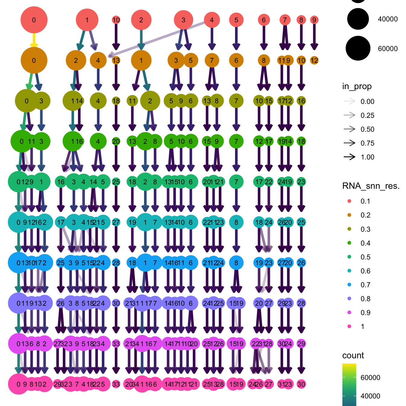
| Version | Author | Date |
|---|---|---|
| 4cbf4d0 | Gunjan Dixit | 2024-12-17 |
p1 <- DimPlot(merged_obj, reduction = "umap.harmony", raster = FALSE ,repel = TRUE, label = TRUE,label.size = 3.5, group.by = "RNA_snn_res.0.6") + NoLegend()Based on the clustering tree, we chose an intermediate/optimum resolution where the clustering results are the most stable, with the least amount of shuffling cells.
opt_res <- "RNA_snn_res.0.6"
n <- nlevels(merged_obj$RNA_snn_res.0.6)
merged_obj$RNA_snn_res.0.6 <- factor(merged_obj$RNA_snn_res.0.6, levels = seq(0,n-1))
merged_obj$seurat_clusters <- NULL
merged_obj$cluster <- merged_obj$RNA_snn_res.0.6
Idents(merged_obj) <- merged_obj$cluster
UMAP after clustering
Defining colours for each cell-type to be consistent with other age-related/cell type composition plots.
my_colors <- c(
  "B cells" = "steelblue",
  "CD4 T cells" = "brown",
  "Double negative T cells" = "gold",
  "CD8 T cells" = "lightgreen",
  "Pre B/T cells" = "orchid",
  "Innate lymphoid cells" = "tan",
  "Natural Killer cells" = "blueviolet",
  "Macrophages" = "green4",
  "Cycling T cells" = "turquoise",
  "Dendritic cells" = "grey80",
  "Gamma delta T cells" = "mediumvioletred",
  "Epithelial lineage" = "darkorange",
  "Granulocytes" = "olivedrab",
  "Fibroblast lineage" = "lavender",
  "None" = "white",
  "Monocytes" = "peachpuff",
  "Endothelial lineage" = "cadetblue",
  "SMG duct" = "lightpink",
  "Neuroendocrine" = "skyblue",
  "Doublet query/Other" = "#d62728"
)
# Define custom colors
custom_colors <- list()
colors_1 <- c(
  '#FFC312', '#C4E538', '#12CBC4', '#FDA7DF', '#ED4C67',
  "lavender", '#A3CB38', '#1289A7', '#D980FA', '#B53471',
  '#EE5A24', '#009432', '#0652DD','#9980FA', "#E5C494",'#833471',
  '#EA2027', '#006266', '#1B1464', '#5758BB', '#6F1E51'
)

colors_2 <- c(
  "darkorange", '#cc8e35', '#ffe119', '#4363d8', '#ffda79',
  '#911eb4', '#42d4f4', '#f032e6', '#bfef45', 'grey90',
  '#469990', '#dcbeff', '#9A6324', '#fffac8', '#800000',
  '#aaffc3', '#808000', '#ffd8b1', '#000075', '#a9a9a9',  "#FB8072"
)


custom_colors$discrete <- c(colors_1, colors_2)
UMAP displaying clusters at opt_res resolution and Broad
cell Labels Level 3.
p1 <- DimPlot(merged_obj, reduction = "umap.harmony", raster = FALSE ,repel = TRUE, label = TRUE,label.size = 3.5, group.by = opt_res) +  NoLegend()

p2 <- DimPlot(merged_obj, reduction = "umap.harmony", raster = FALSE, repel = TRUE, label = TRUE, label.size = 3.5, group.by = "Broad_cell_label_3") +
  scale_colour_manual(values = my_colors) +
  ggtitle(paste0(tissue, ": Batch Corrected UMAP"))


p1 / p2 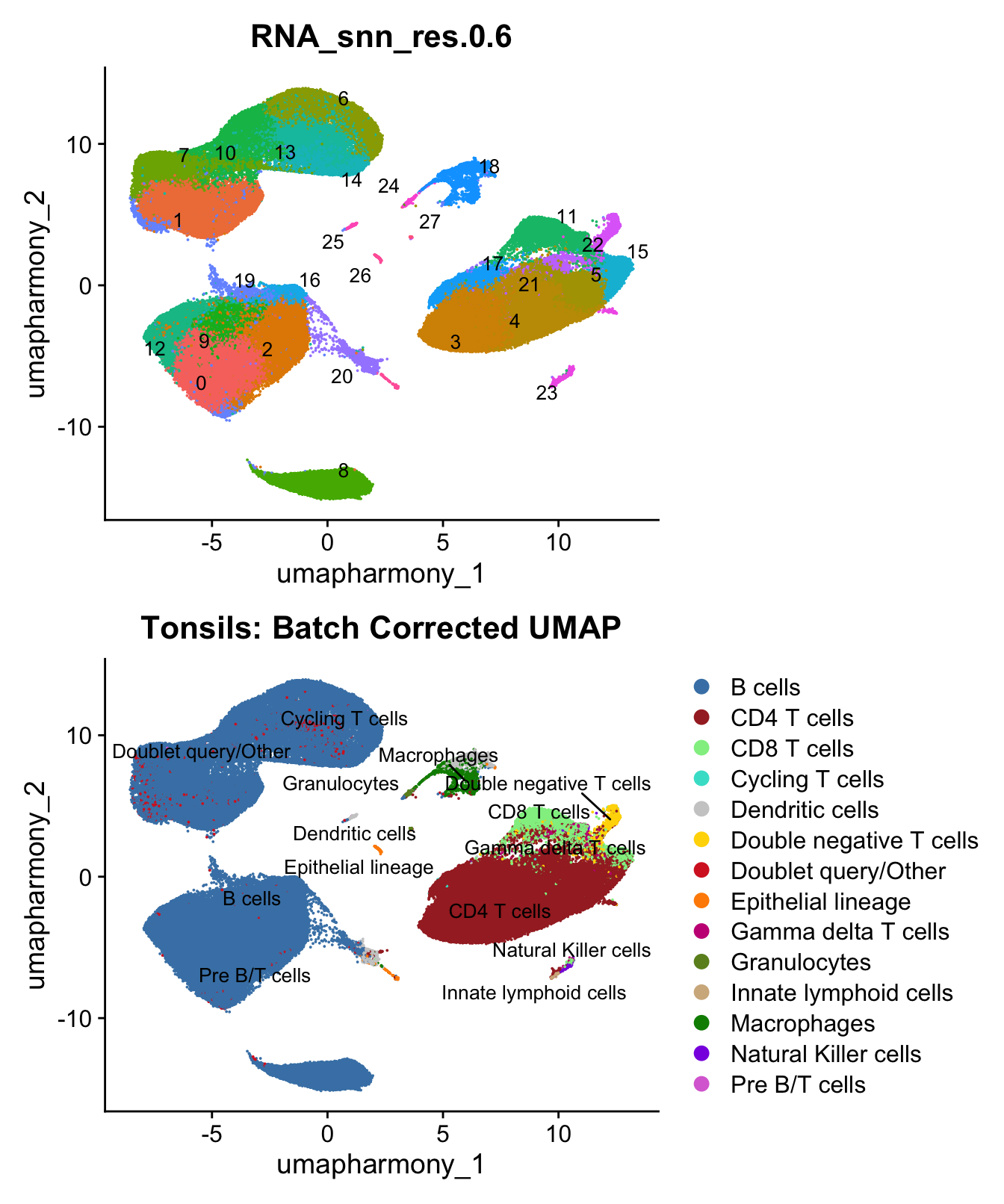
| Version | Author | Date |
|---|---|---|
| 4cbf4d0 | Gunjan Dixit | 2024-12-17 |
p3 <- DimPlot(merged_obj, reduction = "umap.harmony", raster = FALSE, repel = TRUE, label = TRUE, label.size = 3.5, group.by = "predicted.celltype.l1") + NoLegend()
p3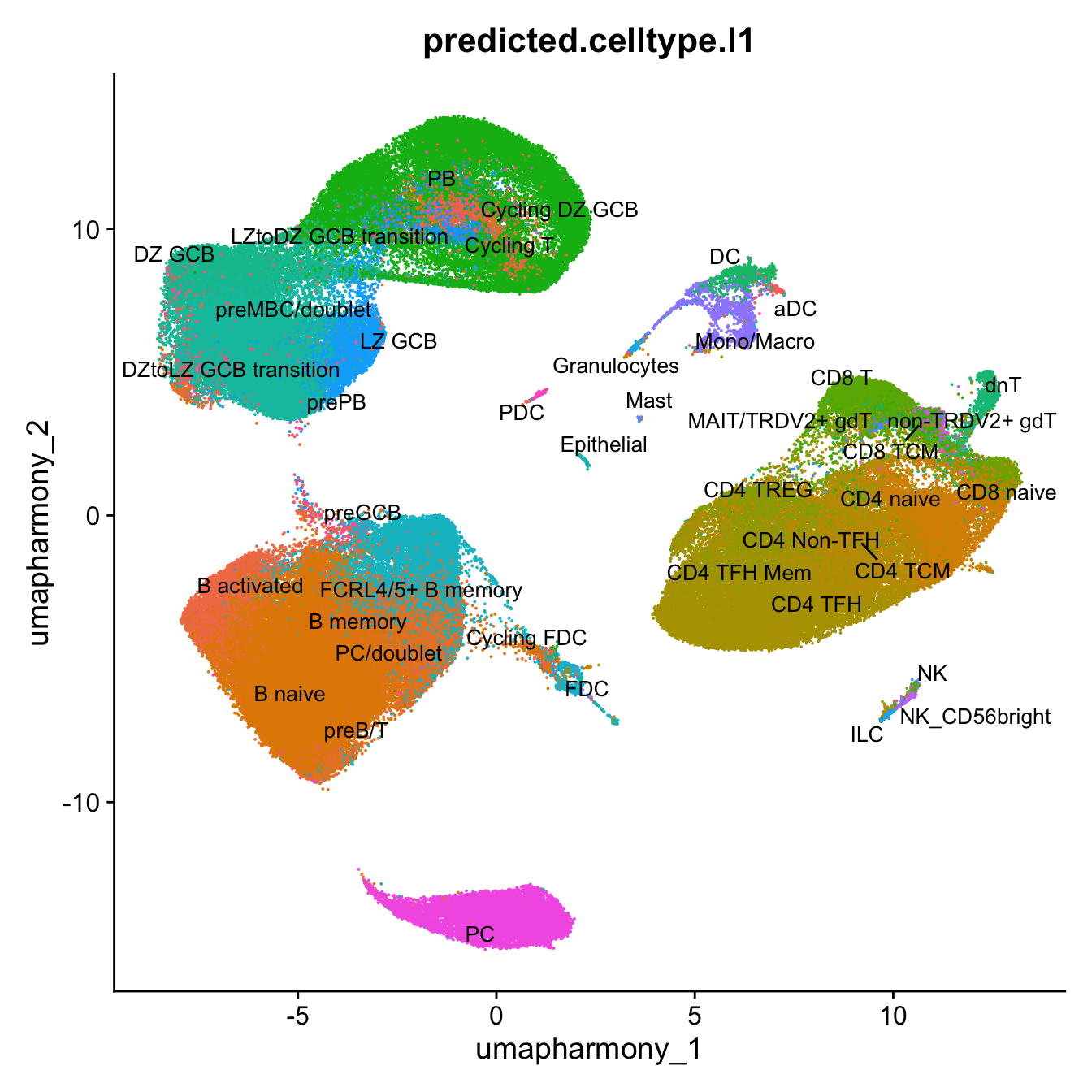
| Version | Author | Date |
|---|---|---|
| 4cbf4d0 | Gunjan Dixit | 2024-12-17 |
p4 <- DimPlot(merged_obj, reduction = "umap.harmony", raster = FALSE, repel = TRUE, label = TRUE, label.size = 3.5, group.by = "predicted.celltype.l2") + NoLegend()
p4
Warning: ggrepel: 42 unlabeled data points (too many overlaps). Consider
increasing max.overlaps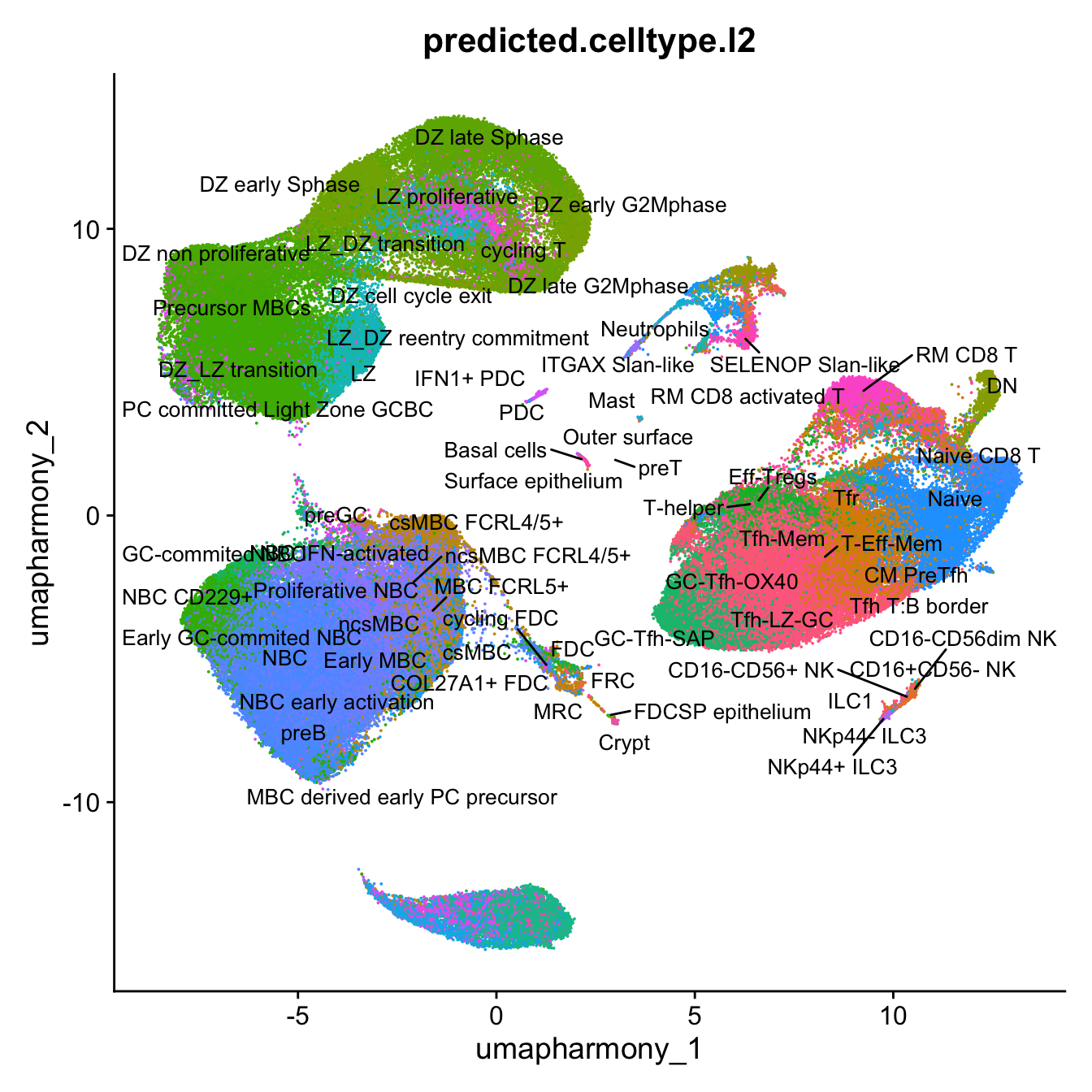
| Version | Author | Date |
|---|---|---|
| 4cbf4d0 | Gunjan Dixit | 2024-12-17 |
p1 <- merged_obj@meta.data %>%
  ggplot(aes(x = !!sym(opt_res),
             fill = !!sym(opt_res))) +
  geom_bar() +
  geom_text(aes(label = ..count..), stat = "count",
            vjust = -0.5, colour = "black", size = 2) +
  scale_y_log10() +
  theme(axis.text.x = element_text(angle = 90,
                                   vjust = 0.5,
                                   hjust = 1,
                                   size = 8)) +
  NoLegend() +
  labs(y = "No. Cells (log scale)")

p2 <- merged_obj@meta.data %>%
  dplyr::select(!!sym(opt_res), predicted.celltype.l1) %>%
  group_by(!!sym(opt_res), predicted.celltype.l1) %>%
  summarise(num = n()) %>%
  mutate(prop = num / sum(num)) %>%
  ggplot(aes(x = !!sym(opt_res), y = prop * 100,
             fill = predicted.celltype.l1)) +
  geom_bar(stat = "identity") +
  theme(axis.text.x = element_text(angle = 90,
                                   vjust = 0.5,
                                   hjust = 1,
                                   size = 8)) +
  labs(y = "% Cells", fill = "predicted.celltype.l1") +
  scale_fill_manual(values = custom_colors$discrete) #+
`summarise()` has grouped output by 'RNA_snn_res.0.6'. You can override using
the `.groups` argument. # paletteer::scale_fill_paletteer_d("ggsci::default_igv")
p3 <- merged_obj@meta.data %>%
dplyr::select(!!sym(opt_res), Broad_cell_label_3) %>%
group_by(!!sym(opt_res), Broad_cell_label_3) %>%
summarise(num = n()) %>%
mutate(prop = num / sum(num)) %>%
ggplot(aes(x = !!sym(opt_res), y = prop * 100,
fill = Broad_cell_label_3)) +
geom_bar(stat = "identity") +
theme(axis.text.x = element_text(angle = 90,
vjust = 0.5,
hjust = 1,
size = 8)) +
labs(y = "% Cells", fill = "Sample") +
scale_fill_manual(values = my_colors) `summarise()` has grouped output by 'RNA_snn_res.0.6'. You can override using
the `.groups` argument.# Combine the plots
(p1 / p2 / p3 ) & theme(legend.text = element_text(size = 8),
legend.key.size = unit(3, "mm"))
| Version | Author | Date |
|---|---|---|
| 4cbf4d0 | Gunjan Dixit | 2024-12-17 |
This table shows Azimuth Level 2 predicted cell types and their counts in each cluster in descending order.
cluster_ids <- sort(unique(merged_obj$cluster))
cluster_celltype_counts <- list()

for (cluster_id in cluster_ids) {
  cluster_data <- merged_obj@meta.data[merged_obj$cluster == cluster_id, ]
  table_counts <- table(cluster_data$predicted.celltype.l2)
  sorted_table <- table_counts[order(-table_counts)]
  cluster_celltype_counts[[as.character(cluster_id)]] <- sorted_table
}

cluster_celltype_counts
$`0`
NBC NBC early activation
21253 15740
ncsMBC Early GC-commited NBC
793 405
ncsMBC FCRL4/5+ Early MBC
178 109
csMBC GC-commited NBC
72 63
MBC FCRL5+ preGC
28 20
MBC derived early PC precursor Precursor MBCs
11 5
NBC IFN-activated NBC CD229+
4 3
DZ_LZ transition Reactivated proliferative MBCs
1 1
$`1`
DZ_LZ transition LZ
18651 3060
LZ_DZ reentry commitment Precursor MBCs
411 340
DZ non proliferative Early MBC
129 32
NBC NBC early activation
26 19
ncsMBC ncsMBC FCRL4/5+
19 16
GC-commited NBC PC committed Light Zone GCBC
9 5
csMBC MBC FCRL5+
3 3
csMBC FCRL4/5+ Early GC-commited NBC
2 2
NBC IFN-activated preGC
2 2
LZ proliferative
1
$`2`
ncsMBC FCRL4/5+ ncsMBC
4509 3511
csMBC NBC
2789 2769
csMBC FCRL4/5+ MBC FCRL5+
1409 1352
NBC early activation Early MBC
837 426
Early GC-commited NBC GC-commited NBC
106 89
preGC Precursor MBCs
47 45
DZ_LZ transition MBC derived early PC precursor
9 8
NBC CD229+ Reactivated proliferative MBCs
4 4
LZ LZ_DZ reentry commitment
1 1
$`3`
Tfh-LZ-GC GC-Tfh-SAP Tfh-Mem GC-Tfh-OX40 Eff-Tregs
6155 4776 3064 1036 262
T-helper T-Eff-Mem CM PreTfh Eff-Tregs-IL32 CM Pre-non-Tfh
176 162 97 67 11
Tfh T:B border T-Trans-Mem Tfr
11 4 3
$`4`
CM PreTfh Tfh-LZ-GC
4873 3618
CM Pre-non-Tfh Naive
1735 1040
Eff-Tregs-IL32 Tfh-Mem
944 913
T-Eff-Mem T-Trans-Mem
601 189
Eff-Tregs T-helper
146 141
Tfh T:B border Tfr
67 44
CM CD8 T GC-Tfh-SAP
41 40
DN SCM CD8 T
32 24
GC-Tfh-OX40 cycling T
14 8
GC-commited NBC NKp44+ ILC3
4 4
TCRVδ+ gd T preGC
4 3
MAIT/CD161+TRDV2+ gd T-cells Naive CD8 T
2 2
RM CD8 T CD16-CD56+ NK
2 1
IFN+ CD8 T RM CD8 activated T
1 1
$`5`
Naive CM Pre-non-Tfh CM PreTfh GC-Tfh-OX40
8580 558 336 307
Tfh-LZ-GC Eff-Tregs-IL32 Naive CD8 T Tfr
96 87 36 29
Eff-Tregs T-Eff-Mem DN Tfh-Mem
26 23 22 15
cycling T TCRVδ+ gd T T-Trans-Mem SCM CD8 T
12 9 3 2
T-helper CD8 Tf CM CD8 T GC-Tfh-SAP
2 1 1 1
RM CD8 activated T
1
$`6`
DZ late Sphase DZ early G2Mphase
7118 2276
LZ proliferative LZ_DZ transition
315 91
DZ early Sphase DZ late G2Mphase
37 35
Reactivated proliferative MBCs LZ_DZ reentry commitment
8 6
LZ cycling FDC
5 3
PB DZ cell cycle exit
2 1
MBC derived early PC precursor
1
$`7`
DZ non proliferative DZ_LZ transition DZ cell cycle exit
6006 2384 386
Precursor MBCs DZ early Sphase LZ
317 11 8
preB Early MBC DZ late G2Mphase
6 4 3
NBC IFN-activated DZ late Sphase NBC early activation
2 1 1
preGC
1
$`8`
IgG+ PC precursor preMature IgG+ PC
4703 1300
Mature IgG+ PC Short lived IgM+ PC
746 537
Mature IgA+ PC MBC derived IgA+ PC
379 349
MBC derived IgG+ PC NBC
283 217
preMature IgM+ PC IgM+ PC precursor
142 131
IgD PC precursor MBC derived early PC precursor
87 61
csMBC PB
53 40
Mature IgM+ PC MBC FCRL5+
34 28
PB committed early PC precursor DZ migratory PC precursor
19 2
Early PC precursor IgM+ early PC precursor
2 2
PC committed Light Zone GCBC preGC
2 2
CM PreTfh Precursor MBCs
1 1
$`9`
NBC NBC IFN-activated
3445 1988
NBC early activation ncsMBC FCRL4/5+
711 705
ncsMBC csMBC FCRL4/5+
280 68
csMBC Early GC-commited NBC
39 32
Early MBC GC-commited NBC
27 22
MBC FCRL5+ Naive
16 2
Precursor MBCs preGC
2 2
CM PreTfh DZ non proliferative
1 1
MBC derived early PC precursor Reactivated proliferative MBCs
1 1
$`10`
DZ early Sphase DZ_LZ transition
4693 999
DZ non proliferative LZ proliferative
371 275
DZ late Sphase LZ
196 177
LZ_DZ reentry commitment DZ cell cycle exit
163 39
Precursor MBCs LZ_DZ transition
31 28
DZ late G2Mphase Reactivated proliferative MBCs
18 13
GC-commited NBC ncsMBC FCRL4/5+
7 2
FDC MBC derived early PC precursor
1 1
NBC
1
$`11`
RM CD8 activated T RM CD8 T
2034 1326
CM CD8 T TCRVδ+ gd T
664 559
SCM CD8 T MAIT/CD161+TRDV2+ gd T-cells
301 285
DN Naive
240 169
CM Pre-non-Tfh Tfh-LZ-GC
167 156
CD8 Tf IFN+ CD8 T
145 126
Naive CD8 T ZNF683+ CD8 T
103 90
DC recruiters CD8 T Eff-Tregs
82 77
T-helper CM PreTfh
71 48
CD16-CD56+ NK CD16+CD56- NK
40 31
Eff-Tregs-IL32 EM CD8 T
29 28
Tfh-Mem CD16-CD56dim NK
18 7
Tfr ILC1
5 4
NKp44+ ILC3 T-Trans-Mem
4 3
GC-Tfh-SAP GC-Tfh-OX40
2 1
$`12`
Early GC-commited NBC GC-commited NBC
2629 1649
NBC NBC early activation
1016 1010
ncsMBC FCRL4/5+ ncsMBC
160 52
csMBC FCRL4/5+ MBC FCRL5+
23 23
Early MBC NBC IFN-activated
21 20
Precursor MBCs NBC CD229+
11 6
csMBC preGC
3 3
MBC derived early PC precursor LZ proliferative
2 1
LZ_DZ reentry commitment Naive
1 1
Reactivated proliferative MBCs
1
$`13`
DZ late Sphase Reactivated proliferative MBCs
1559 989
DZ early Sphase Precursor MBCs
744 552
DZ early G2Mphase LZ proliferative
441 362
LZ_DZ transition DZ_LZ transition
337 186
DZ late G2Mphase NBC
181 149
Early MBC DZ cell cycle exit
126 113
DZ non proliferative cycling T
74 68
LZ_DZ reentry commitment preGC
61 37
MBC derived early PC precursor LZ
36 16
GC-commited NBC ncsMBC FCRL4/5+
15 9
NBC IFN-activated cycling FDC
6 5
MBC FCRL5+ csMBC
5 4
csMBC FCRL4/5+ NBC early activation
3 3
PB preB
3 3
ncsMBC
2
$`14`
DZ late G2Mphase DZ cell cycle exit
3719 350
LZ_DZ transition DZ early G2Mphase
196 165
LZ proliferative DZ early Sphase
126 39
DZ late Sphase DZ_LZ transition
18 17
Reactivated proliferative MBCs LZ
14 10
Precursor MBCs cycling FDC
3 1
DZ non proliferative GC-commited NBC
1 1
LZ_DZ reentry commitment MBC derived early PC precursor
1 1
$`15`
Naive CD8 T Naive CM Pre-non-Tfh SCM CD8 T TCRVδ+ gd T
2291 1807 60 35 35
DN CM PreTfh CM CD8 T Tfr Tfh-LZ-GC
34 24 22 8 7
Eff-Tregs CD8 Tf GC-Tfh-OX40 GC-Tfh-SAP
4 1 1 1
$`16`
csMBC FCRL4/5+ ncsMBC FCRL4/5+
2645 1052
GC-commited NBC NBC
31 31
MBC FCRL5+ Early GC-commited NBC
18 10
NBC IFN-activated ncsMBC
10 9
NBC early activation Early MBC
3 2
Reactivated proliferative MBCs csMBC
2 1
$`17`
Eff-Tregs T-helper
1431 726
Tfh-Mem Eff-Tregs-IL32
510 296
Tfh-LZ-GC GC-Tfh-OX40
156 82
GC-Tfh-SAP Naive
53 44
CM Pre-non-Tfh T-Trans-Mem
22 20
MAIT/CD161+TRDV2+ gd T-cells cycling T
12 11
CM PreTfh T-Eff-Mem
10 10
CM CD8 T DN
6 5
Tfr Naive CD8 T
4 2
NKp44+ ILC3 SCM CD8 T
2 2
CD16+CD56- NK CD8 Tf
1 1
ILC1 RM CD8 activated T
1 1
RM CD8 T TCRVδ+ gd T
1 1
$`18`
SELENOP Slan-like DC2
777 438
MMP Slan-like C1Q Slan-like
326 320
ITGAX Slan-like aDC1
232 144
M1 Macrophages Monocytes
128 118
DC5 DC1 precursor
112 106
DC1 mature DC4
96 54
IL7R DC aDC3
38 31
Neutrophils ncsMBC FCRL4/5+
11 10
Naive preGC
7 7
CM Pre-non-Tfh CM PreTfh
6 6
NBC T-Eff-Mem
4 4
Tfh-LZ-GC Basal cells
4 3
Crypt FDC
3 3
COL27A1+ FDC GC-commited NBC
2 2
RM CD8 activated T csMBC FCRL4/5+
2 1
DZ_LZ transition Eff-Tregs
1 1
Eff-Tregs-IL32 FRC
1 1
MAIT/CD161+TRDV2+ gd T-cells MRC
1 1
Naive CD8 T PDC
1 1
Tfh-Mem
1
$`19`
NBC Early MBC
651 391
preGC DZ_LZ transition
355 326
Precursor MBCs LZ_DZ reentry commitment
223 136
csMBC FCRL4/5+ ncsMBC FCRL4/5+
134 112
GC-commited NBC DZ non proliferative
88 71
MBC FCRL5+ LZ
57 55
MBC derived early PC precursor csMBC
35 26
Reactivated proliferative MBCs preB
19 16
NBC early activation DZ early Sphase
15 6
LZ proliferative DZ cell cycle exit
6 5
NBC IFN-activated ncsMBC
3 3
cycling T Naive
2 2
Proliferative NBC cycling FDC
2 1
GC-Tfh-OX40 LZ_DZ transition
1 1
PC committed Light Zone GCBC
1
$`20`
FDC NBC
385 342
COL27A1+ FDC cycling FDC
238 91
csMBC FCRL4/5+ Early MBC
80 74
ncsMBC FCRL4/5+ DZ_LZ transition
72 66
CD14+CD55+ FDC MRC
41 40
NBC early activation ncsMBC
34 26
MBC FCRL5+ Naive
21 20
Precursor MBCs Crypt
18 15
csMBC Tfh-LZ-GC
14 14
preGC CM PreTfh
10 7
GC-commited NBC Basal cells
7 6
Early GC-commited NBC PDC
6 6
Reactivated proliferative MBCs FRC
6 5
T-helper Eff-Tregs
5 4
LZ_DZ reentry commitment CM Pre-non-Tfh
4 3
DN DZ late Sphase
2 2
Eff-Tregs-IL32 GC-Tfh-SAP
2 2
ITGAX Slan-like SELENOP Slan-like
2 2
Tfh-Mem aDC1
2 1
CD8 Tf CM CD8 T
1 1
DC1 mature DZ early Sphase
1 1
IgG+ PC precursor LZ
1 1
Mature IgA+ PC MBC derived IgG+ PC
1 1
MMP Slan-like Naive CD8 T
1 1
Neutrophils RM CD8 activated T
1 1
SCM CD8 T
1
$`21`
Naive CM Pre-non-Tfh Tfh-LZ-GC Naive CD8 T
518 335 227 109
Tfh-Mem Eff-Tregs CM PreTfh Eff-Tregs-IL32
85 60 53 33
IFN+ CD8 T T-Eff-Mem T-helper cycling T
12 8 6 3
DN RM CD8 activated T SCM CD8 T GC-Tfh-OX40
2 2 2 1
GC-Tfh-SAP NBC IFN-activated T-Trans-Mem
1 1 1
$`22`
DN Naive CM CD8 T CM Pre-non-Tfh
1210 62 21 20
SCM CD8 T Eff-Tregs-IL32 TCRVδ+ gd T CM PreTfh
12 9 7 5
Tfh-LZ-GC CD8 Tf cycling T Naive CD8 T
5 4 3 3
GC-Tfh-OX40 RM CD8 activated T RM CD8 T GC-Tfh-SAP
2 2 2 1
T-Eff-Mem T-helper
1 1
$`23`
CD16-CD56+ NK NKp44+ ILC3
306 230
Naive CD16+CD56- NK
65 63
CD16-CD56dim NK ILC1
56 44
ZNF683+ CD8 T TCRVδ+ gd T
38 32
CM PreTfh CM Pre-non-Tfh
29 23
CM CD8 T MAIT/CD161+TRDV2+ gd T-cells
19 18
T-Trans-Mem Tfh-LZ-GC
14 12
EM CD8 T DC recruiters CD8 T
9 4
RM CD8 activated T T-helper
3 3
DN preT
2 2
Tfh-Mem cycling T
2 1
Eff-Tregs GC-commited NBC
1 1
IFN+ CD8 T Mast
1 1
Naive CD8 T NKp44- ILC3
1 1
SCM CD8 T Tfr
1 1
$`24`
Neutrophils Early GC-commited NBC NBC early activation
451 15 13
preGC NBC M1 Macrophages
13 10 9
CM PreTfh Mast aDC3
6 6 5
ncsMBC FCRL4/5+ C1Q Slan-like Crypt
3 2 2
csMBC FCRL4/5+ Naive NBC IFN-activated
2 2 2
SELENOP Slan-like COL27A1+ FDC csMBC
2 1 1
DC5 Early MBC FDC
1 1 1
GC-Tfh-SAP ncsMBC Precursor MBCs
1 1 1
Tfh-LZ-GC
1
$`25`
PDC NBC GC-commited NBC preGC CM PreTfh
420 3 2 2 1
IFN1+ PDC
1
$`26`
Surface epithelium Outer surface Crypt
125 102 74
preGC FDCSP epithelium Basal cells
60 7 4
NBC SELENOP Slan-like Tfh-LZ-GC
4 2 2
aDC3 C1Q Slan-like CM Pre-non-Tfh
1 1 1
CM PreTfh COL27A1+ FDC Early GC-commited NBC
1 1 1
FDC MRC Naive
1 1 1
NBC early activation NBC IFN-activated ncsMBC FCRL4/5+
1 1 1
$`27`
Mast CM PreTfh
64 2 Save batch corrected Object
out1 <- here("output",
            "RDS", "AllBatches_Clustering_SEUs_v2",
             paste0("G000231_Neeland_",tissue,".Clusters.SEU.rds"))
#dir.create(out1)
saveRDS(merged_obj, file = out1)
Marker Gene Analysis
The marker genes for this reclustering can be found here-
merged_obj <- JoinLayers(merged_obj)
paed.markers <- FindAllMarkers(merged_obj, only.pos = TRUE, min.pct = 0.25, logfc.threshold = 0.25)
Extracting top 5 genes per cluster for visualization. The ‘top5’ contains the top 5 genes with the highest weighted average avg_log2FC within each cluster and the ‘best.wilcox.gene.per.cluster’ contains the single best gene with the highest weighted average avg_log2FC for each cluster.
paed.markers %>%
    group_by(cluster) %>% unique() %>%
    top_n(n = 5, wt = avg_log2FC) -> top5

paed.markers %>%
    group_by(cluster) %>%
    slice_head(n=1) %>%
    pull(gene) -> best.wilcox.gene.per.cluster

best.wilcox.gene.per.cluster
[1] "IGHD" "LMO2" "TNFRSF13B" "MAF" "TCF7" "TCF7"
[7] "KIFC1" "AICDA" "DERL3" "IFI44L" "MCM4" "CCL5"
[13] "FCER2" "TYMS" "CDC20" "CD8A" "FCRL4" "MAF"
[19] "LYZ" "ACTB" "CLU" "IFI44L" "GZMK" "TRDC"
[25] "ITGAX" "CLEC4C" "LCN2" "CPA3" Marker gene expression in clusters
This heatmap depicts the expression of top five genes in each cluster.
DoHeatmap(merged_obj, features = top5$gene) + NoLegend()
| Version | Author | Date |
|---|---|---|
| 4cbf4d0 | Gunjan Dixit | 2024-12-17 |
Violin plot shows the expression of top marker gene per cluster.
VlnPlot(merged_obj, features=best.wilcox.gene.per.cluster, ncol = 2, raster = FALSE, pt.size = FALSE)
| Version | Author | Date |
|---|---|---|
| 4cbf4d0 | Gunjan Dixit | 2024-12-17 |
Violin plot shows the expression of top marker gene per cluster and compares its expression in both batches.
plots <- VlnPlot(merged_obj, features = best.wilcox.gene.per.cluster, split.by = "batch_name", group.by = "Broad_cell_label_3",
    pt.size = 0, combine = FALSE, raster = FALSE, split.plot = TRUE)
The default behaviour of split.by has changed.
Separate violin plots are now plotted side-by-side.
To restore the old behaviour of a single split violin,
set split.plot = TRUE.
This message will be shown once per session.wrap_plots(plots = plots, ncol = 1)
| Version | Author | Date |
|---|---|---|
| 4cbf4d0 | Gunjan Dixit | 2024-12-17 |
Feature plot shows the expression of top marker genes per cluster.
FeaturePlot(merged_obj,features=best.wilcox.gene.per.cluster, reduction = 'umap.harmony', raster = FALSE, ncol = 2)
| Version | Author | Date |
|---|---|---|
| 4cbf4d0 | Gunjan Dixit | 2024-12-17 |
Extract markers for each cluster
This section extracts marker genes for each cluster and save them as a CSV file.
out_markers <- here("output",
"CSV_v2", tissue,
paste(tissue,"_Marker_gene_clusters.",opt_res, sep = ""))
dir.create(out_markers, recursive = TRUE, showWarnings = FALSE)
for (cl in unique(paed.markers$cluster)) {
cluster_data <- paed.markers %>% dplyr::filter(cluster == cl)
file_name <- here(out_markers, paste0("G000231_Neeland_",tissue, "_cluster_", cl, ".csv"))
write.csv(cluster_data, file = file_name)
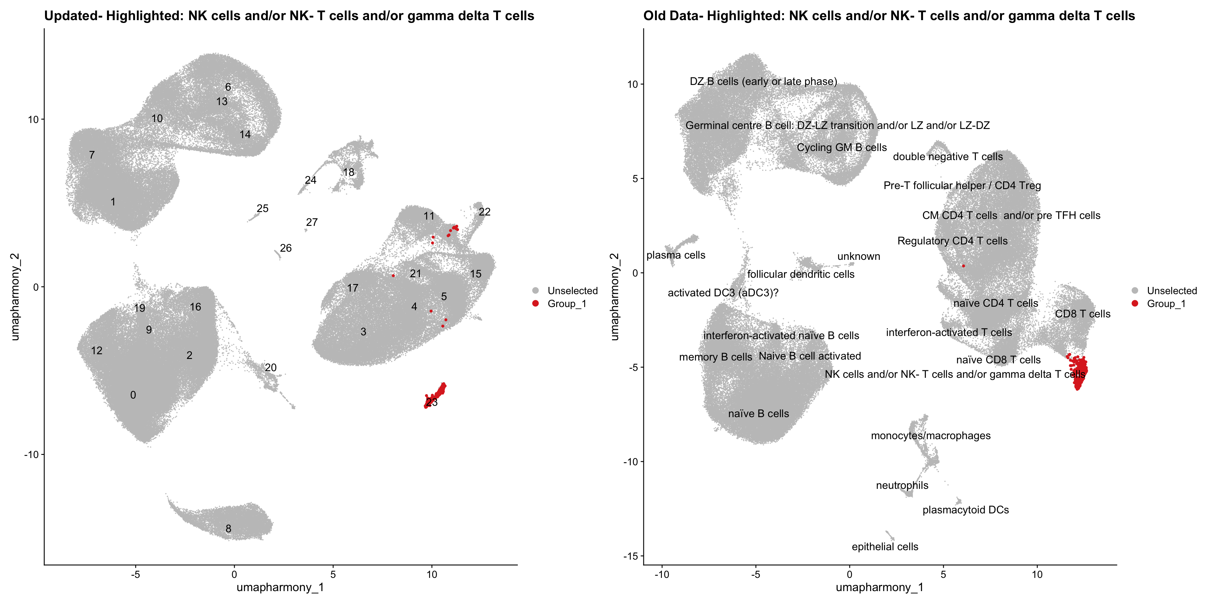
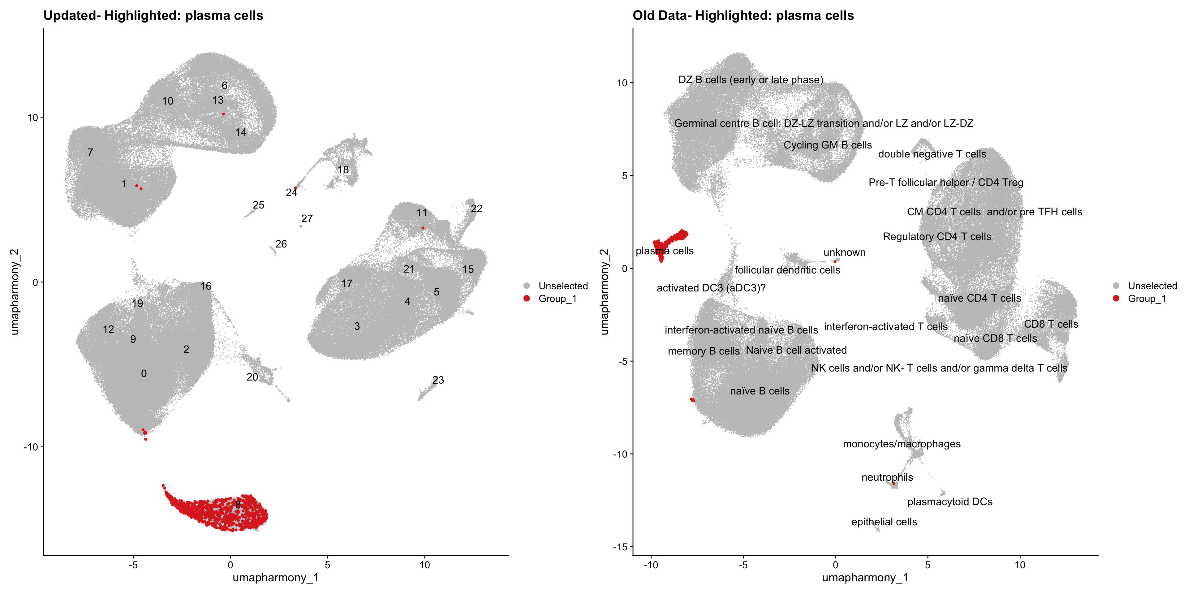
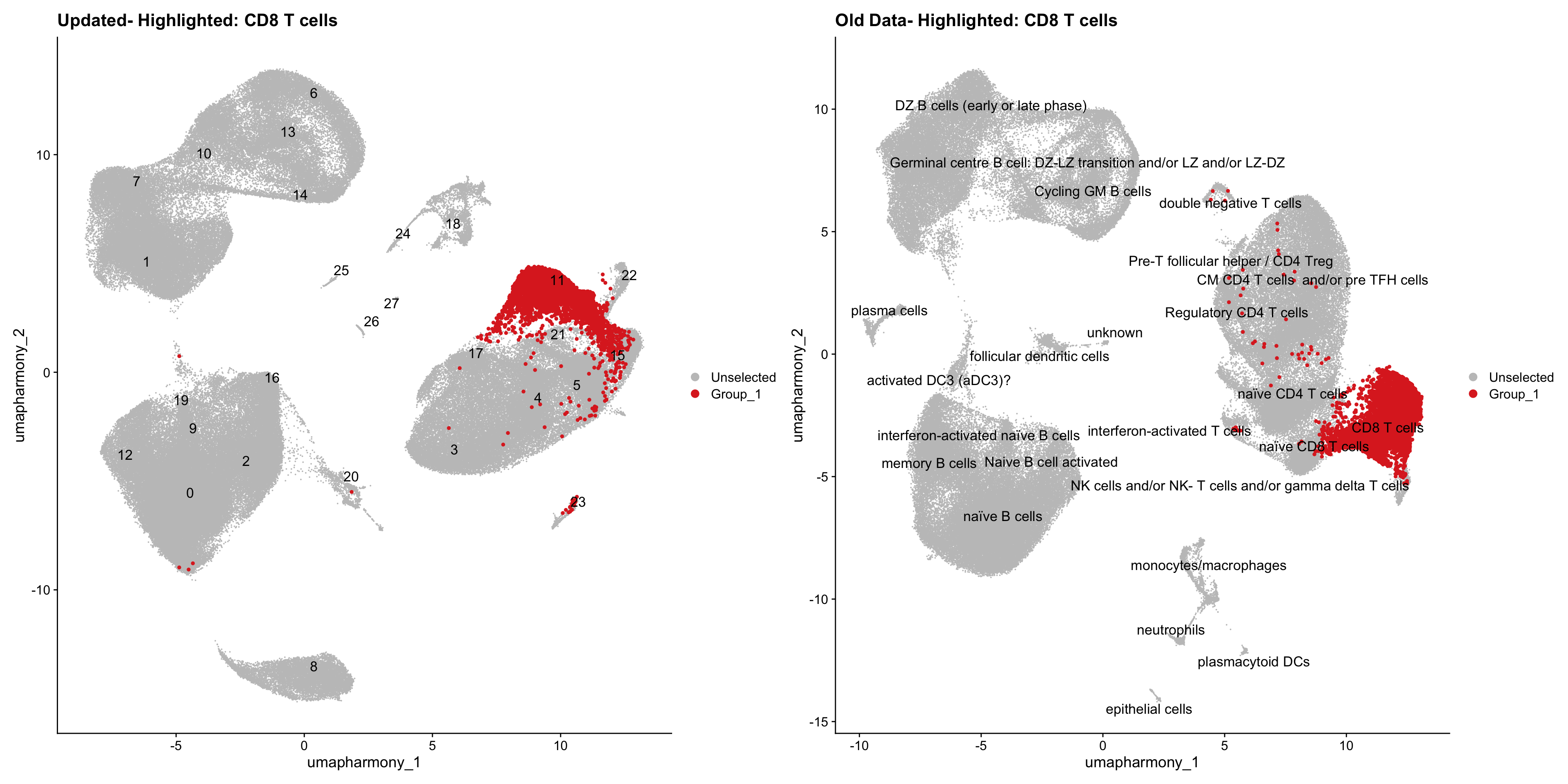
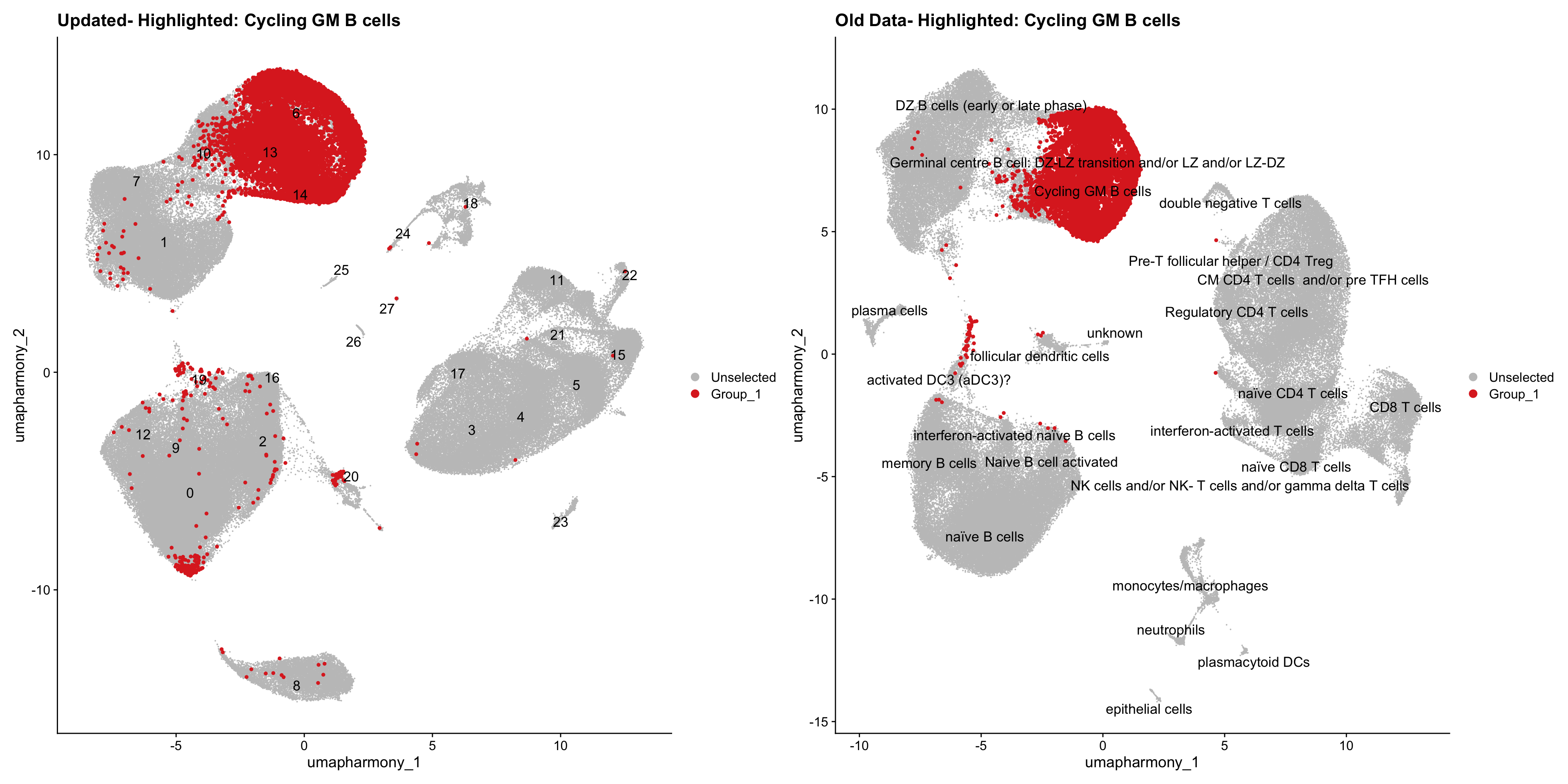
}Using old labels to annotate cell types
out1 <- here("output",
"RDS", "AllBatches_Clustering_SEUs",
paste0("G000231_Neeland_",tissue,".Clusters.SEU.rds"))
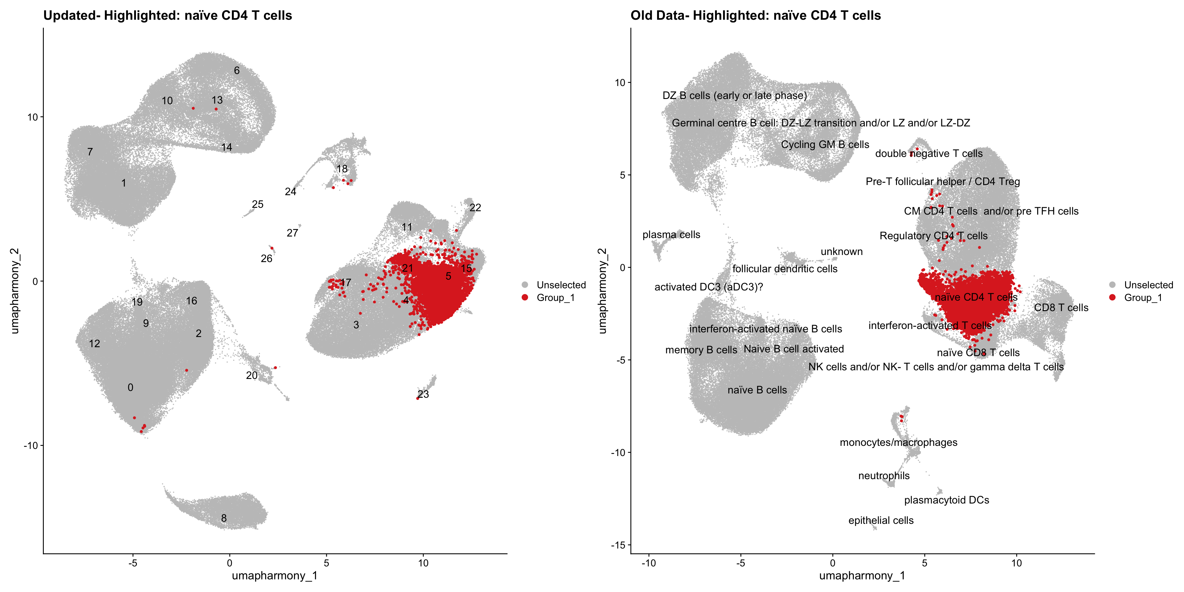
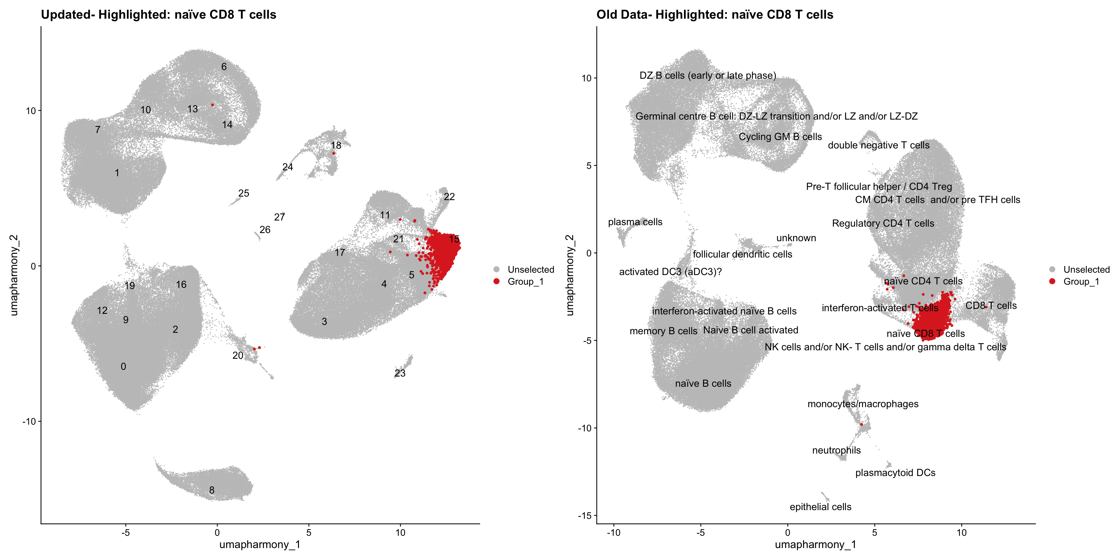
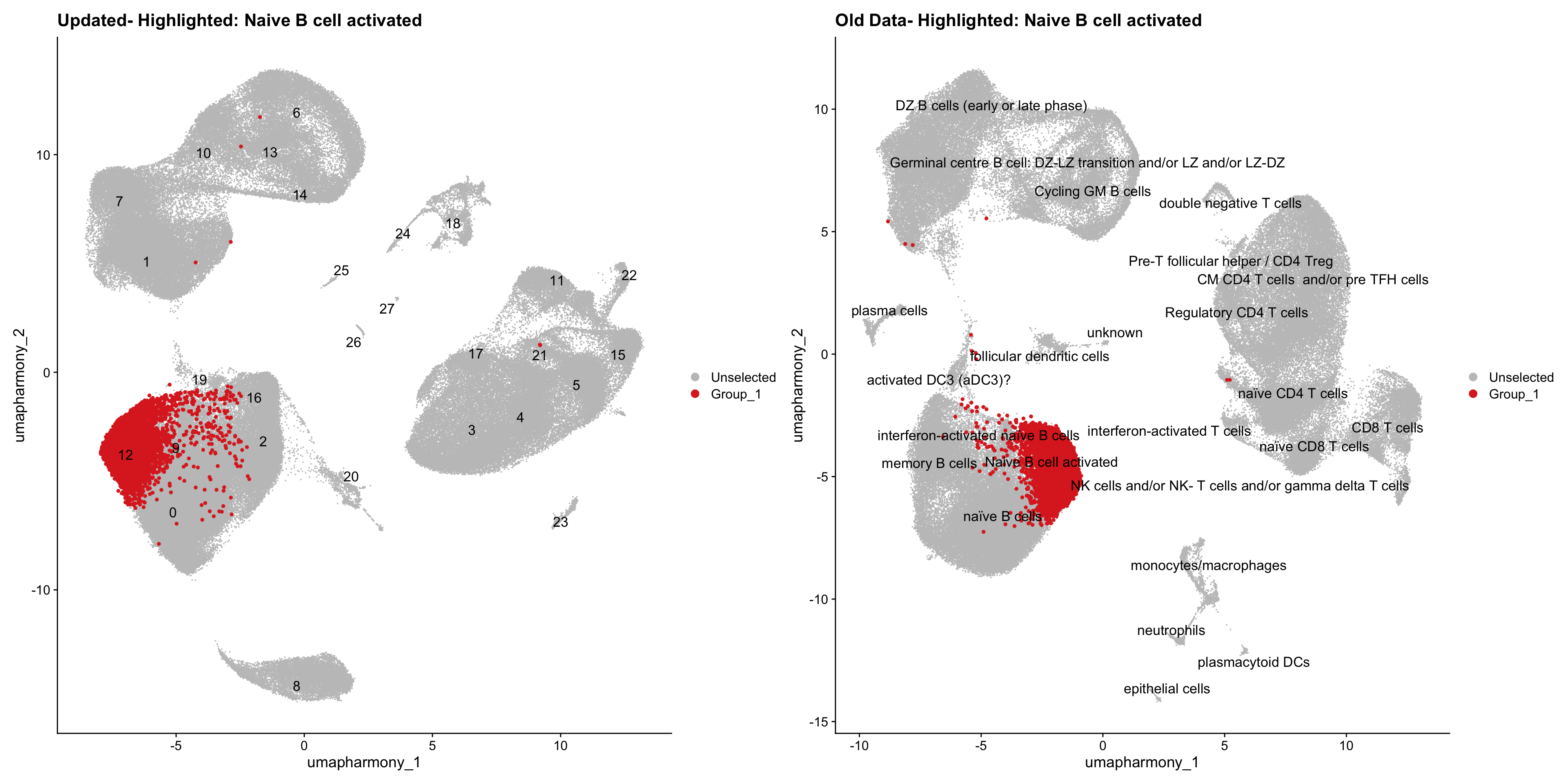
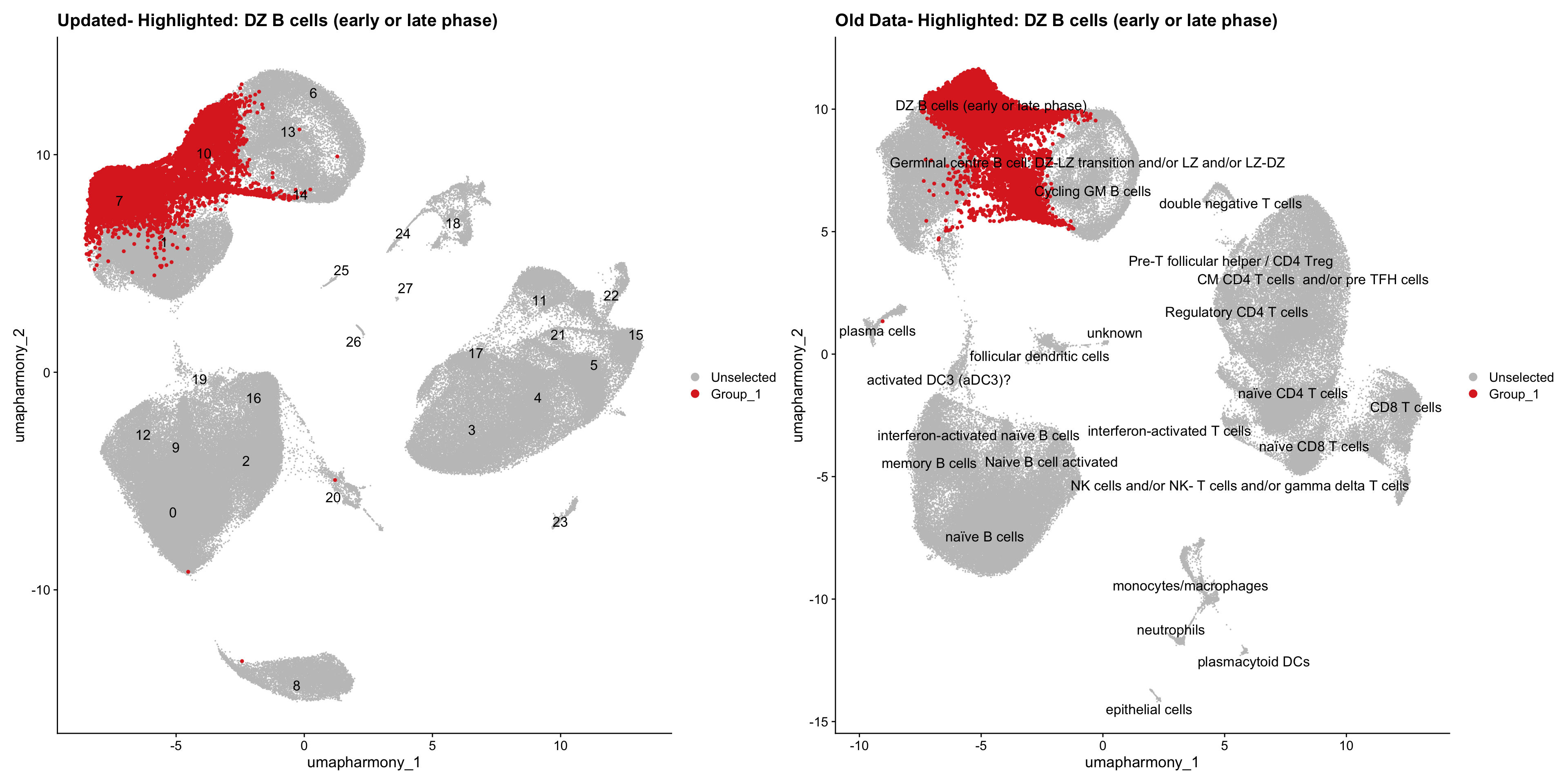
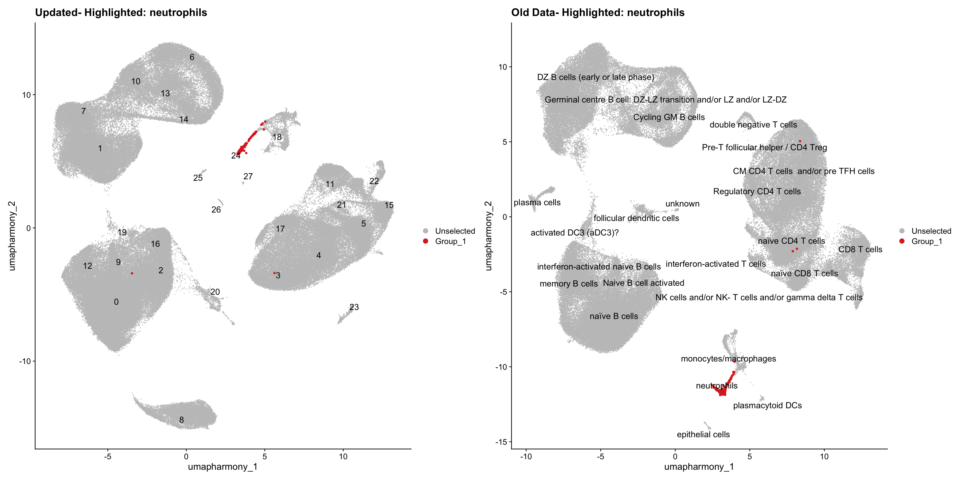
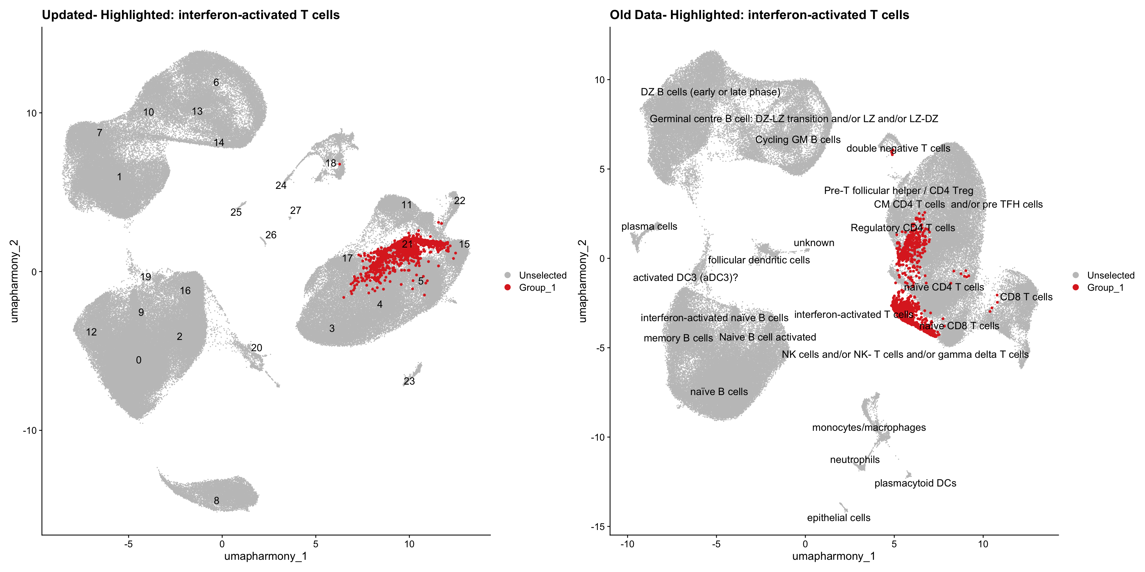
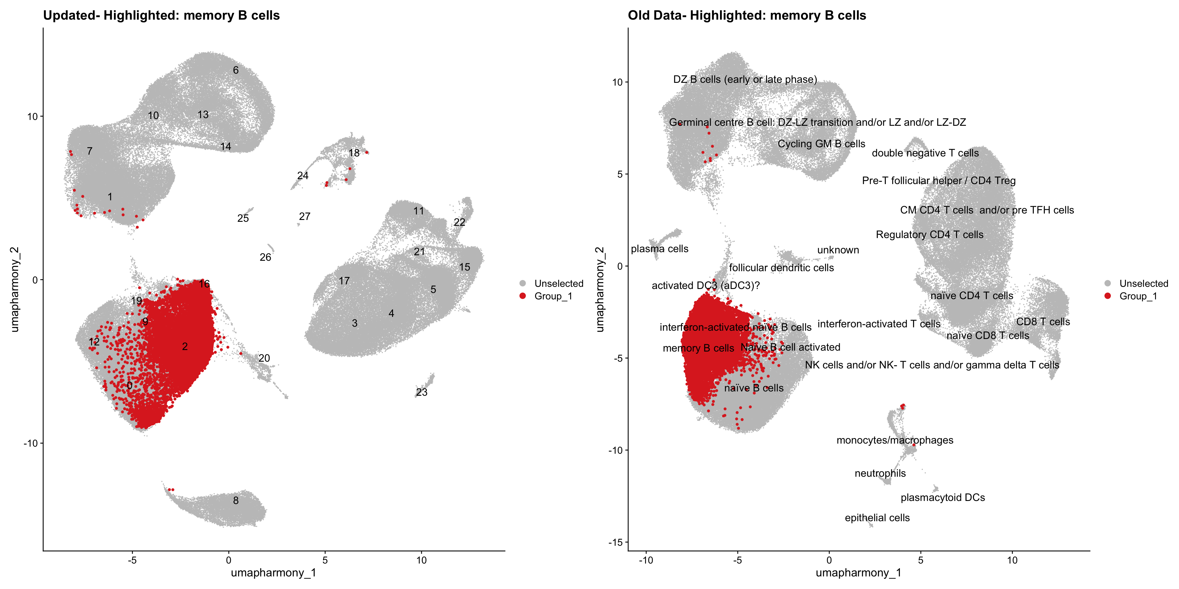
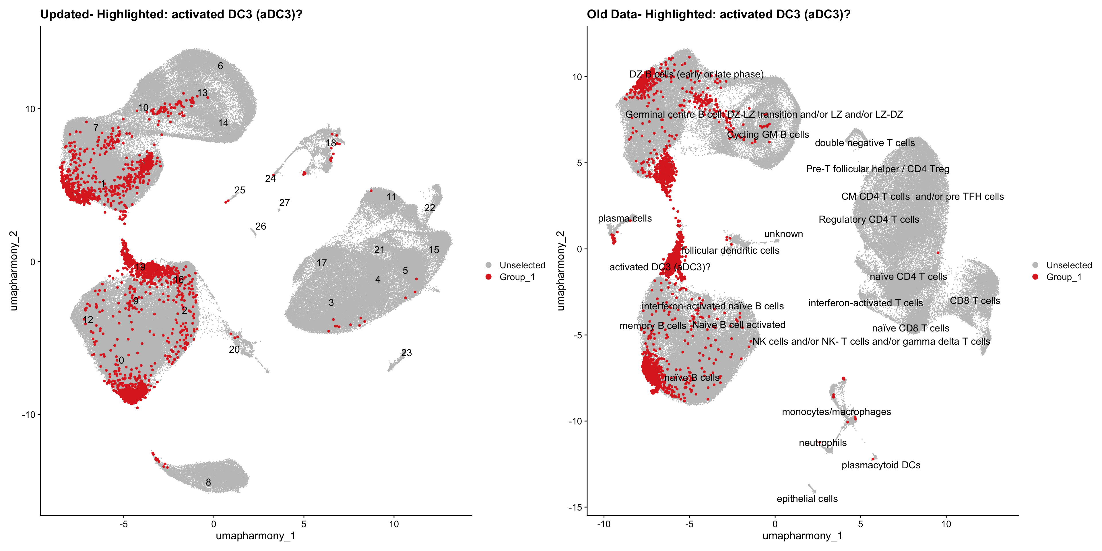
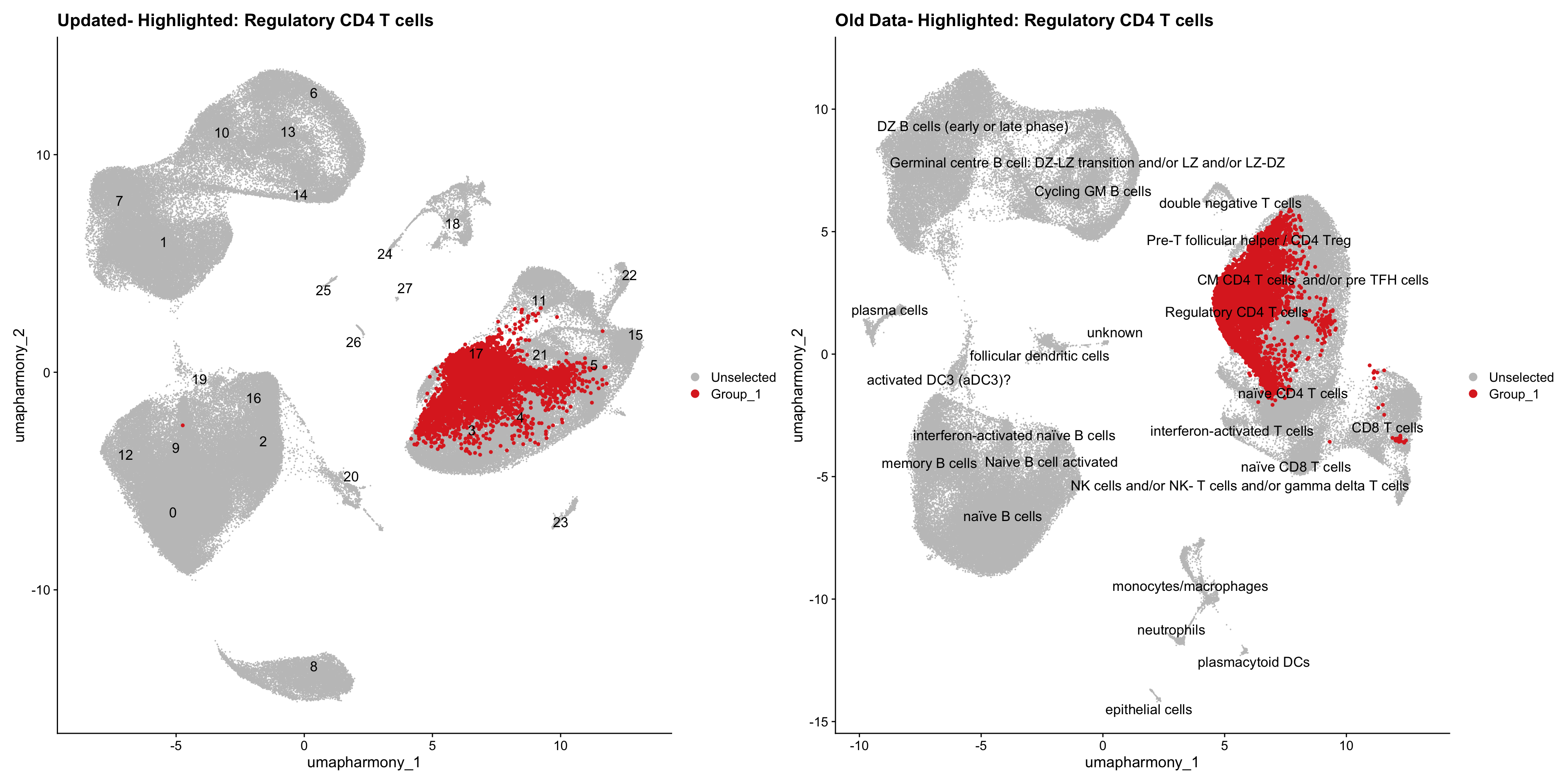
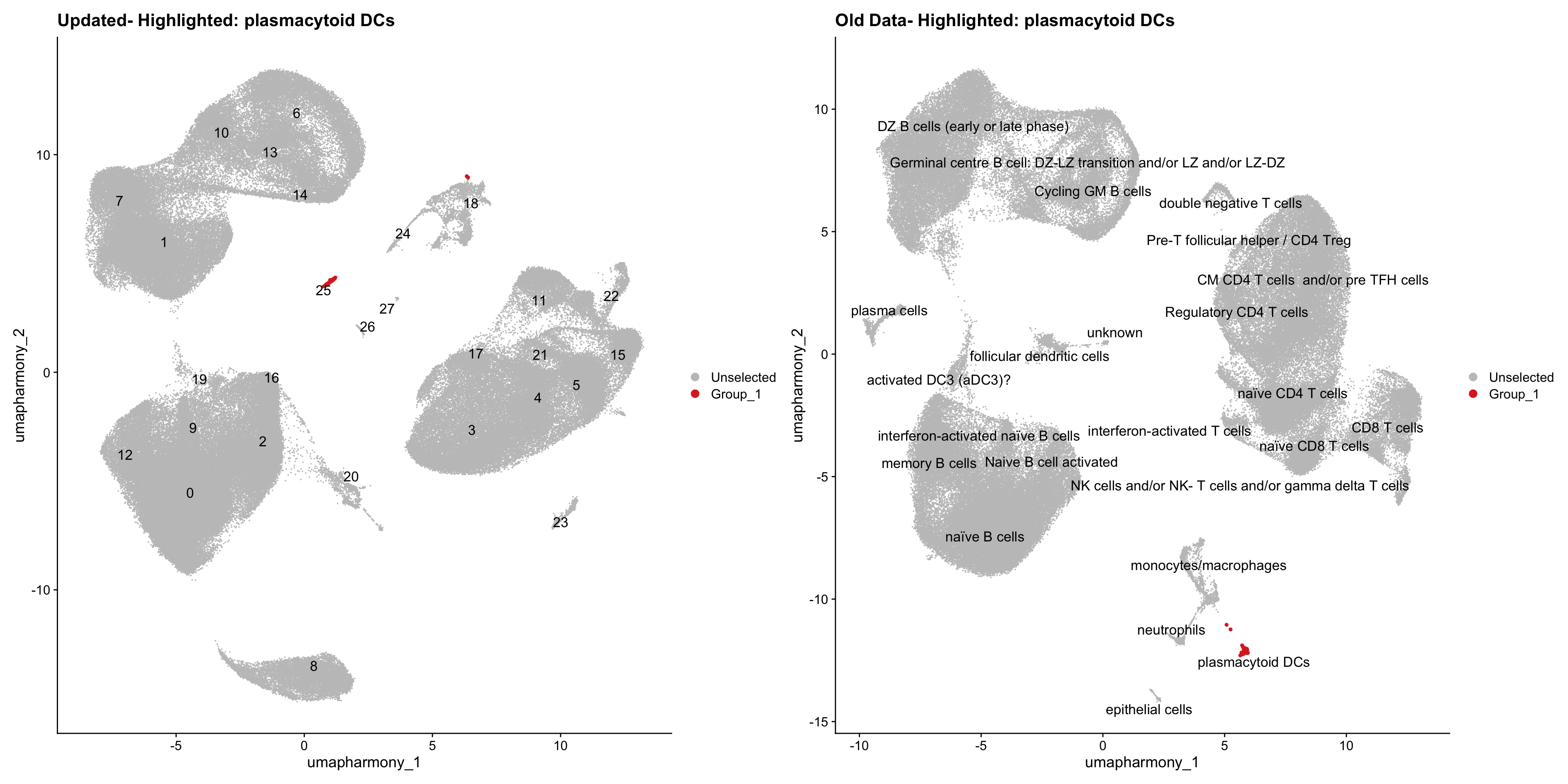
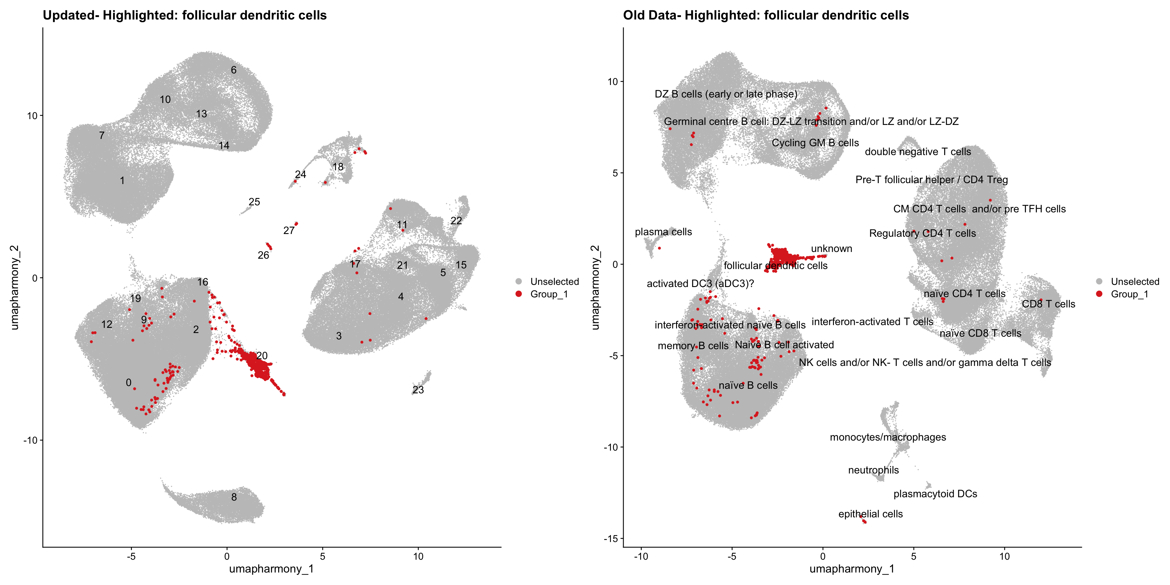
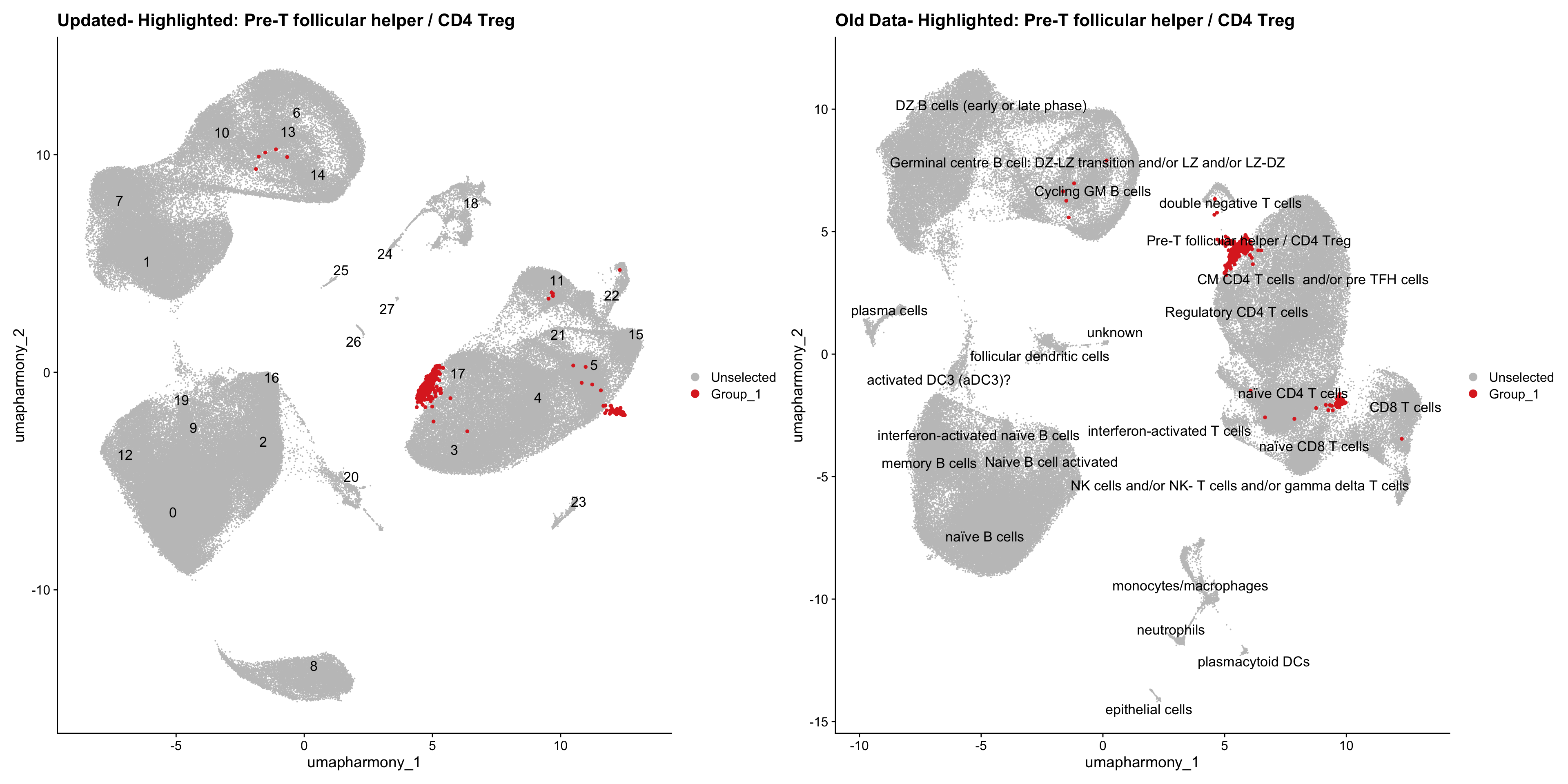
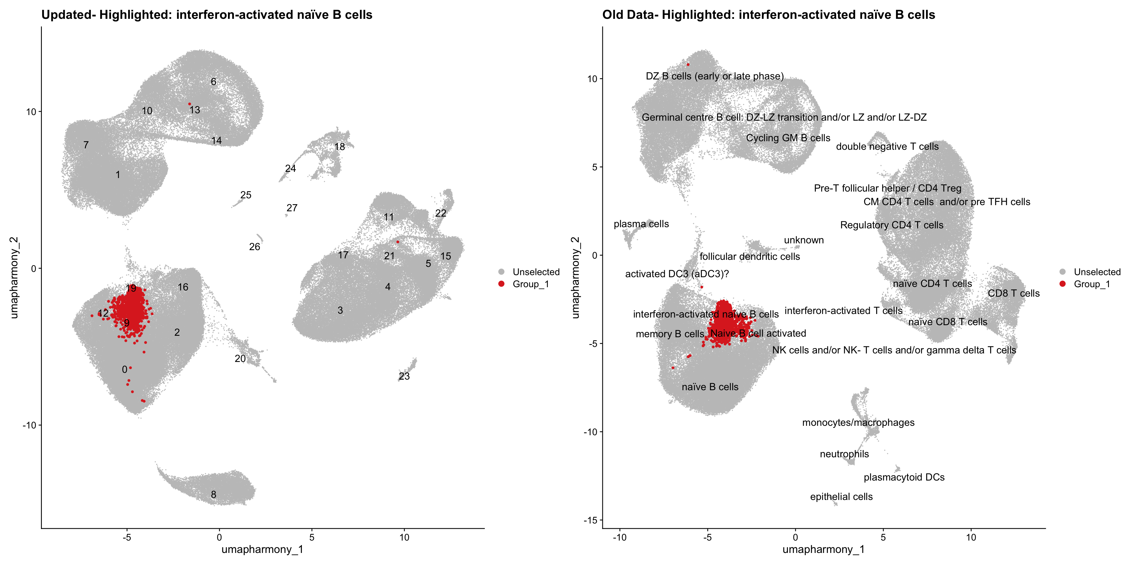
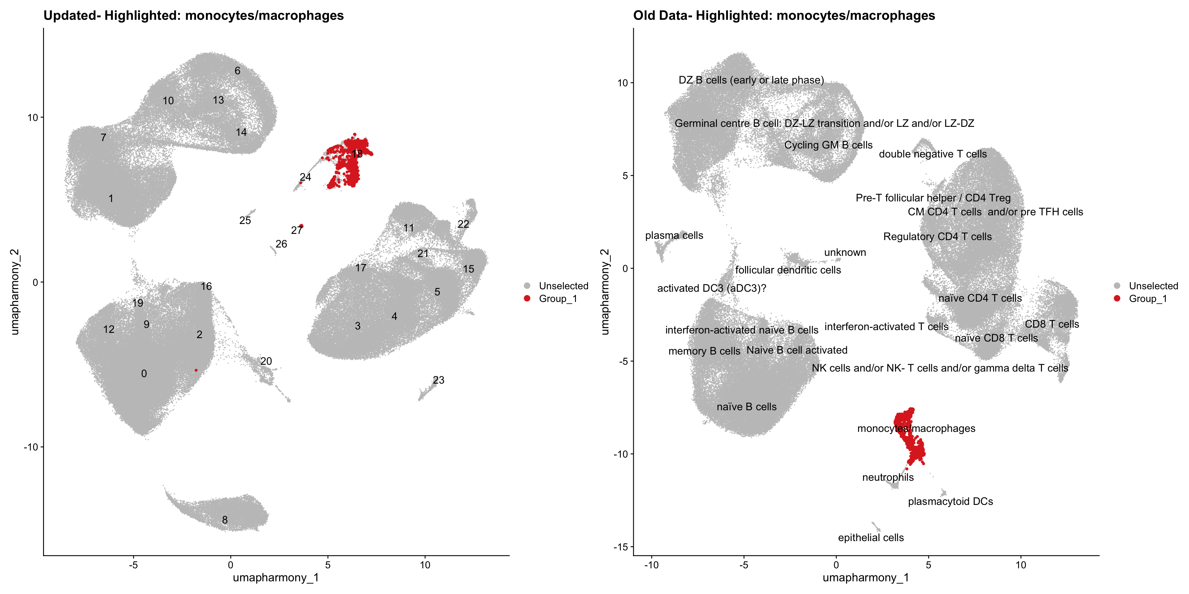
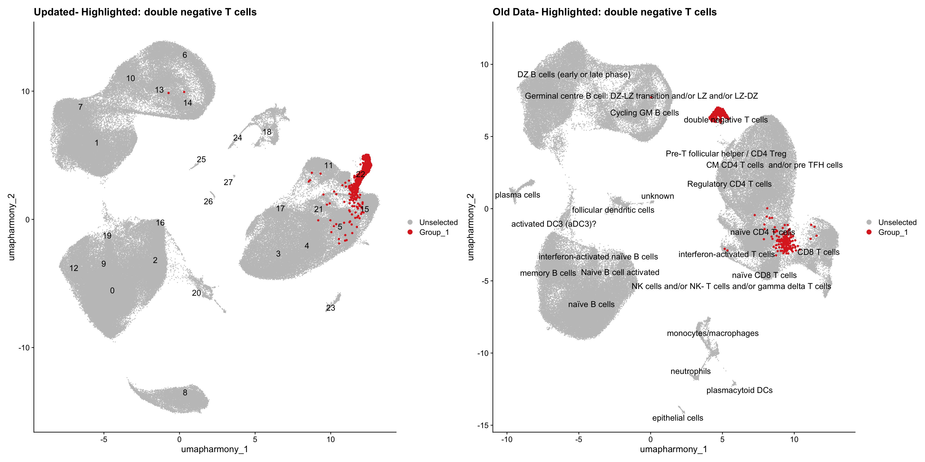
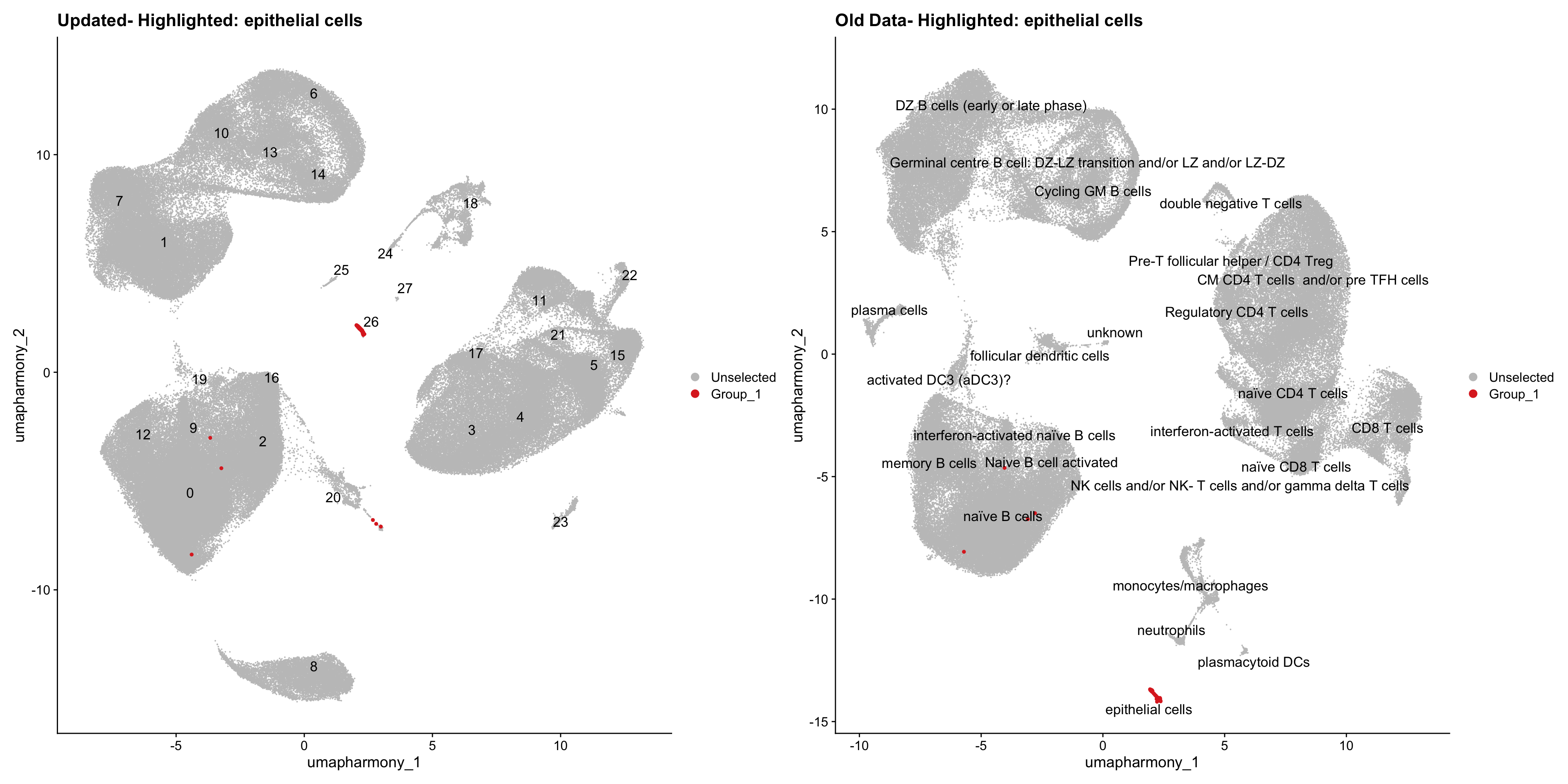
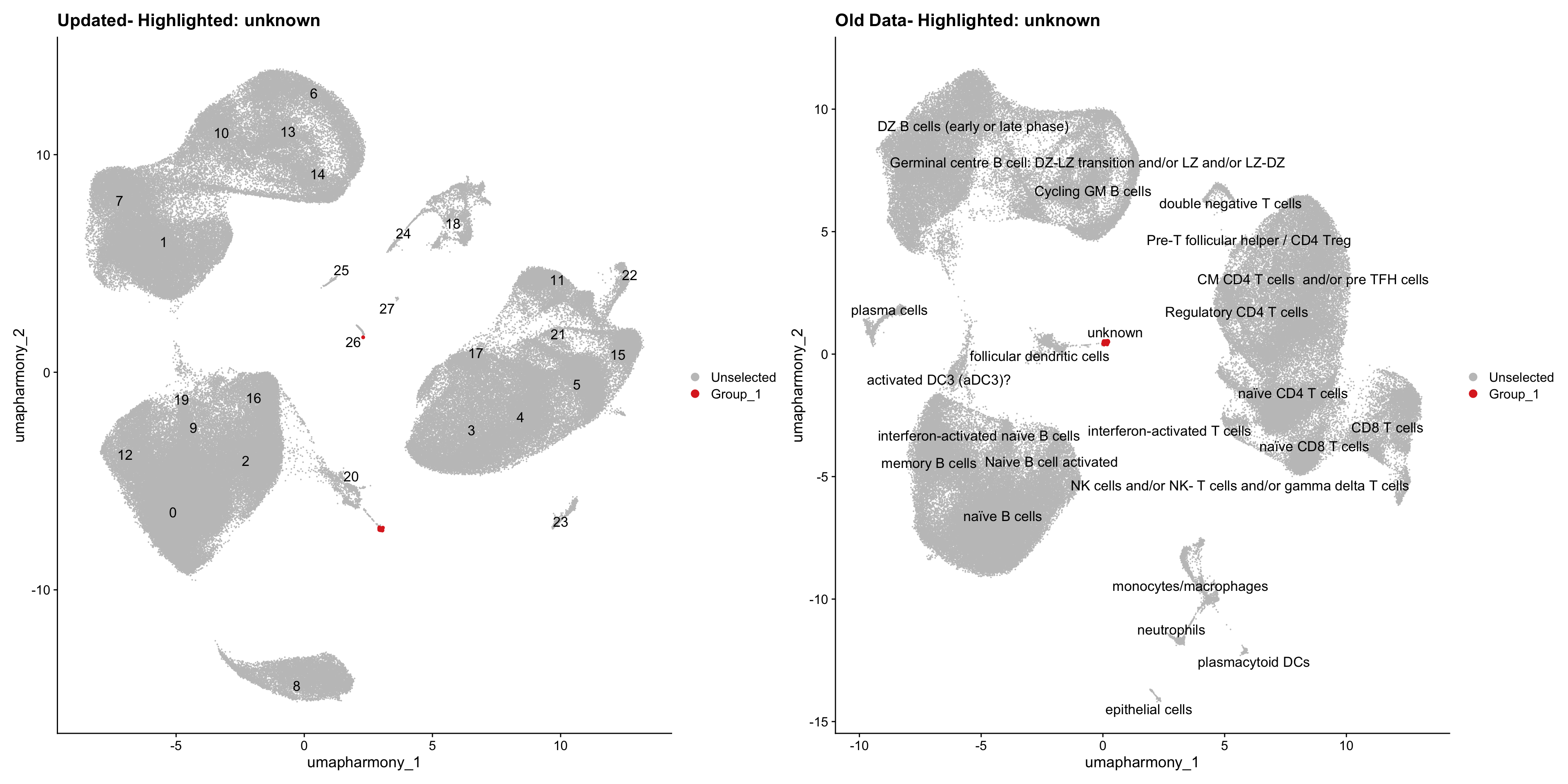
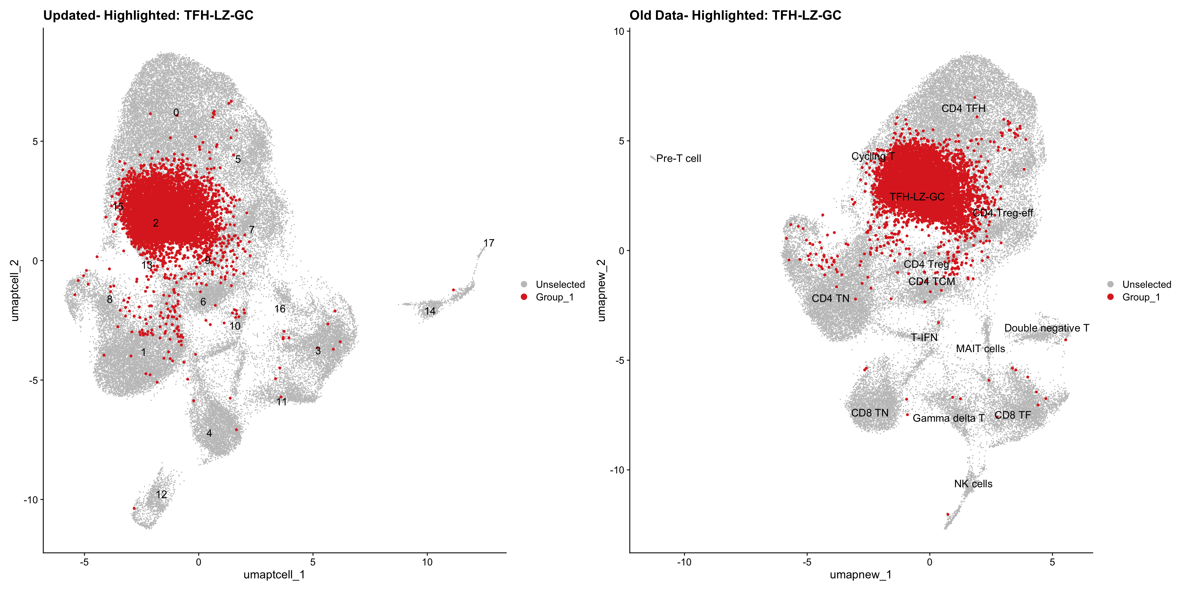
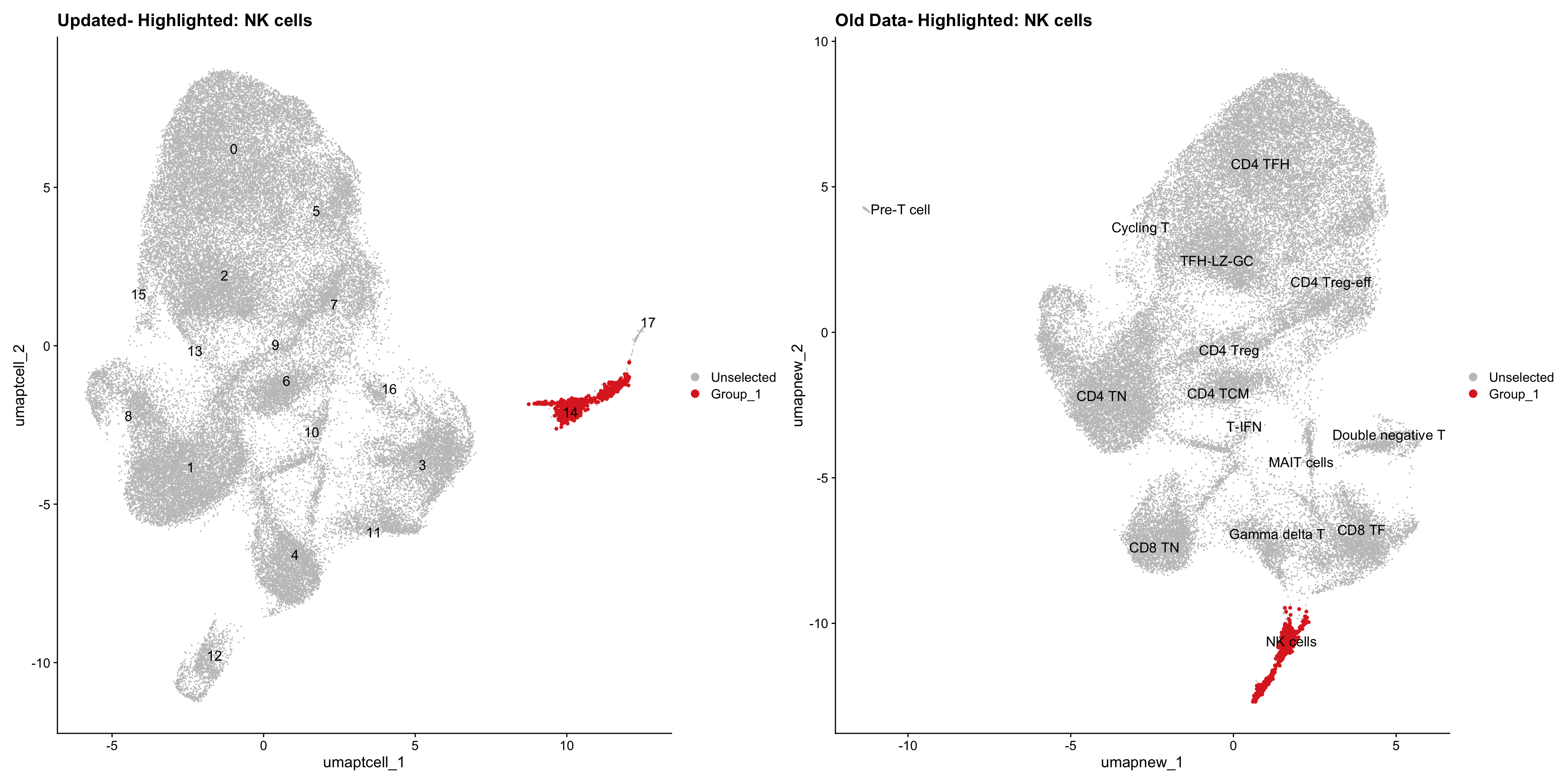
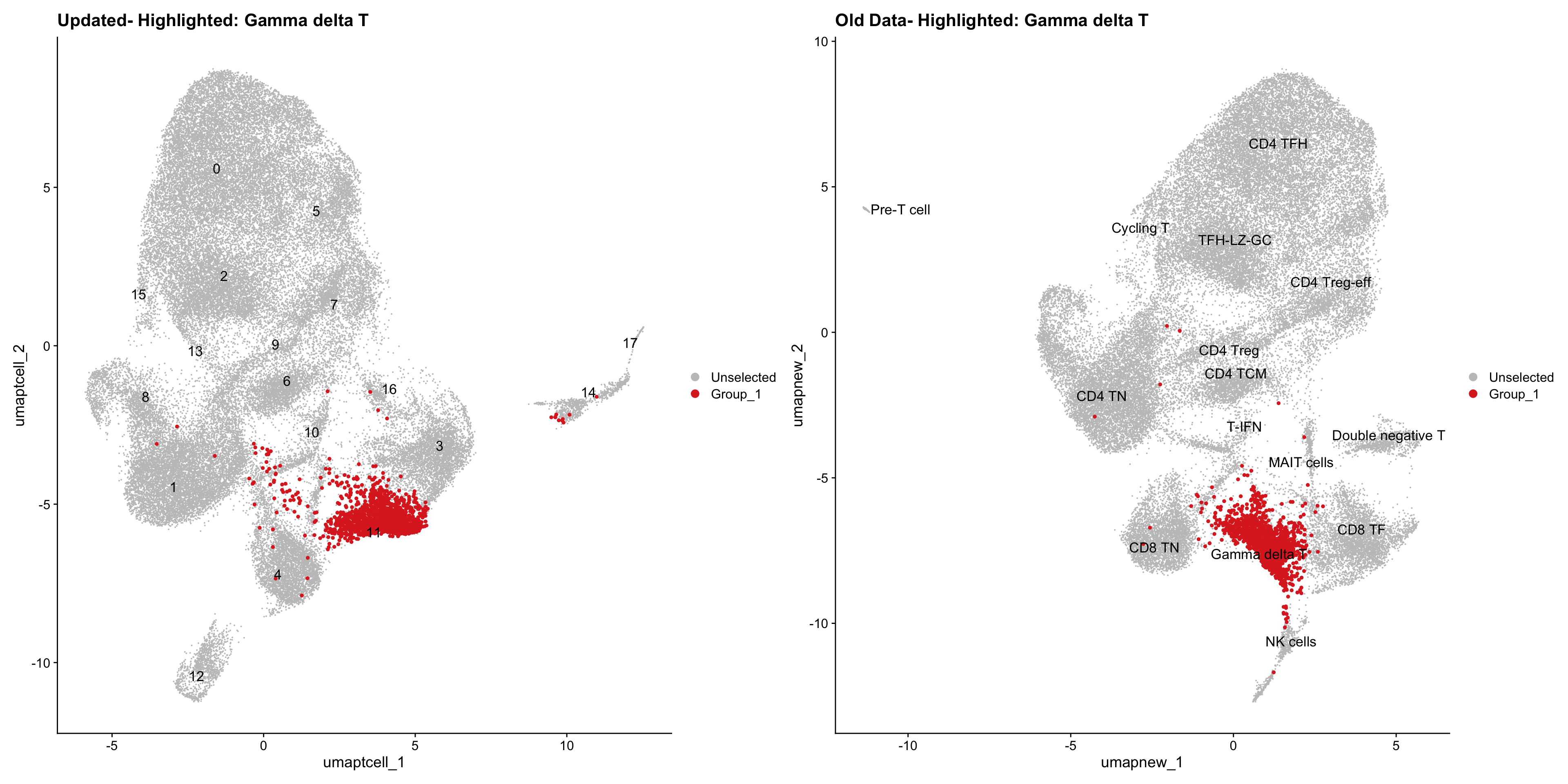
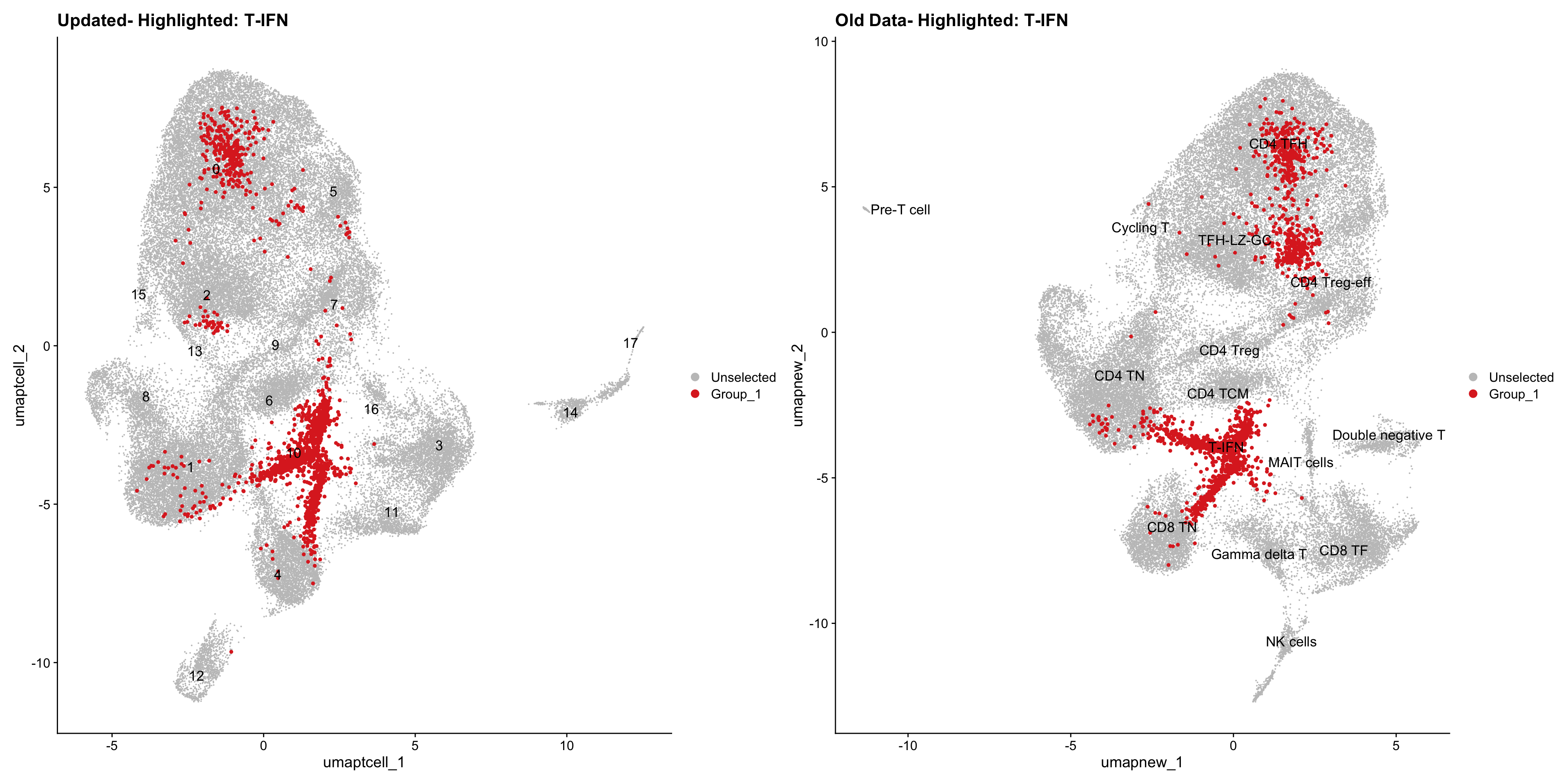
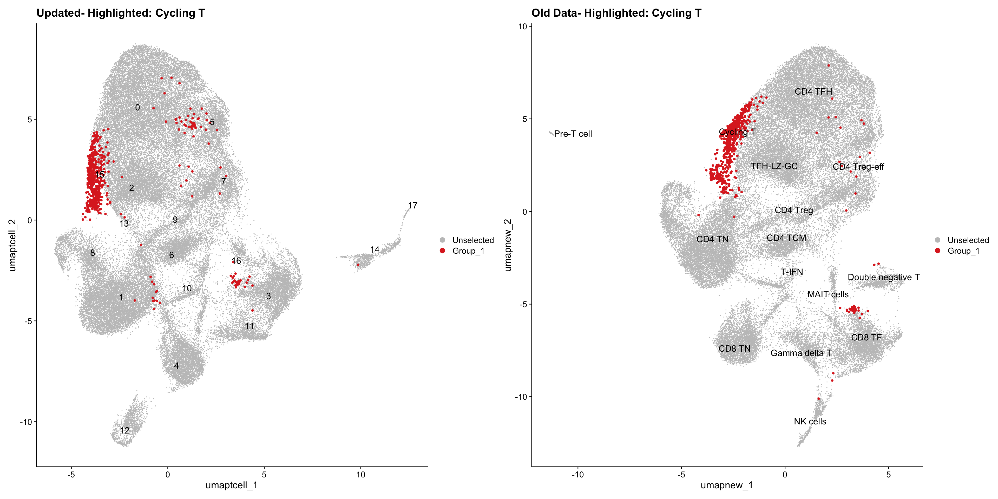
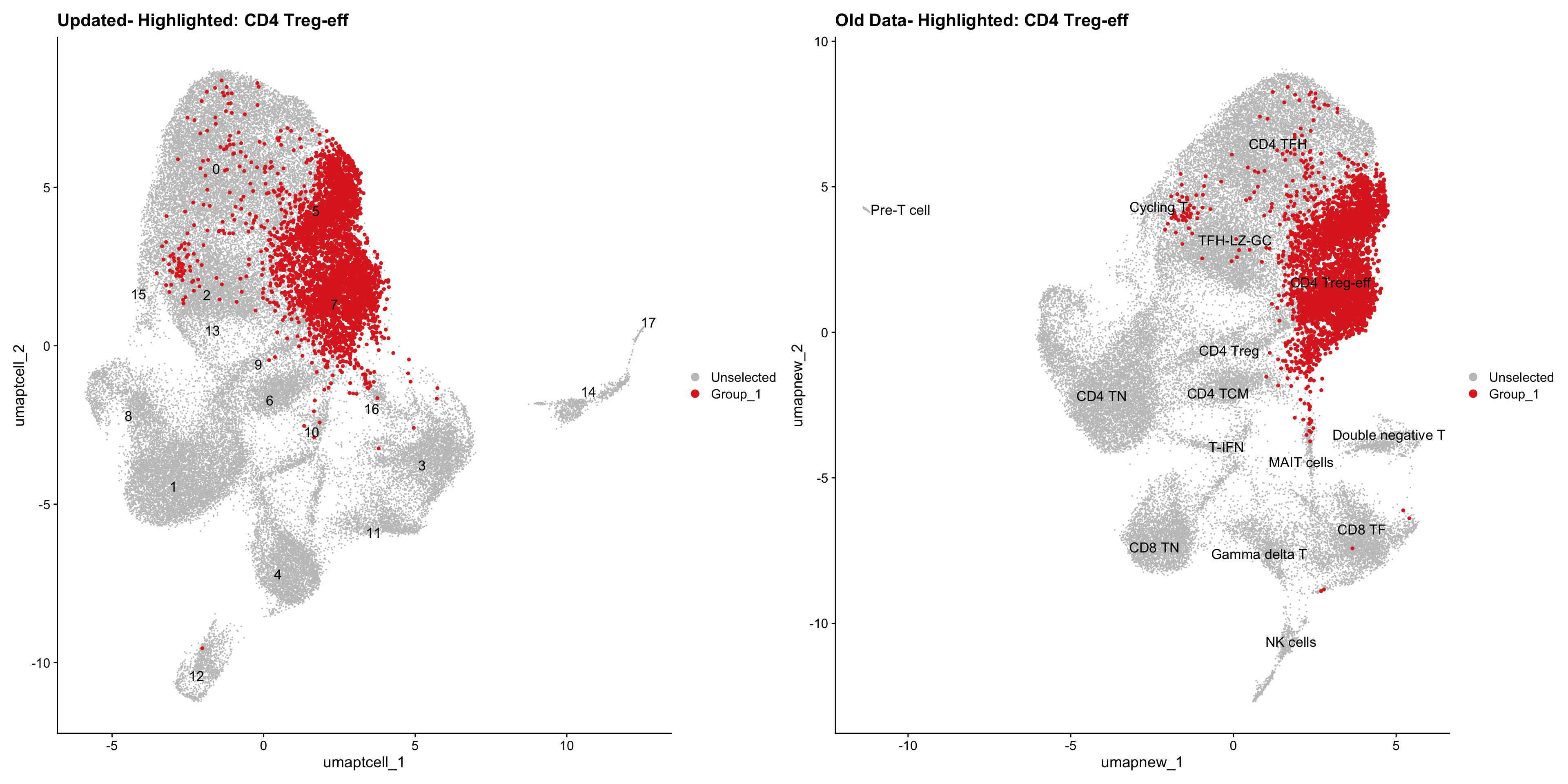
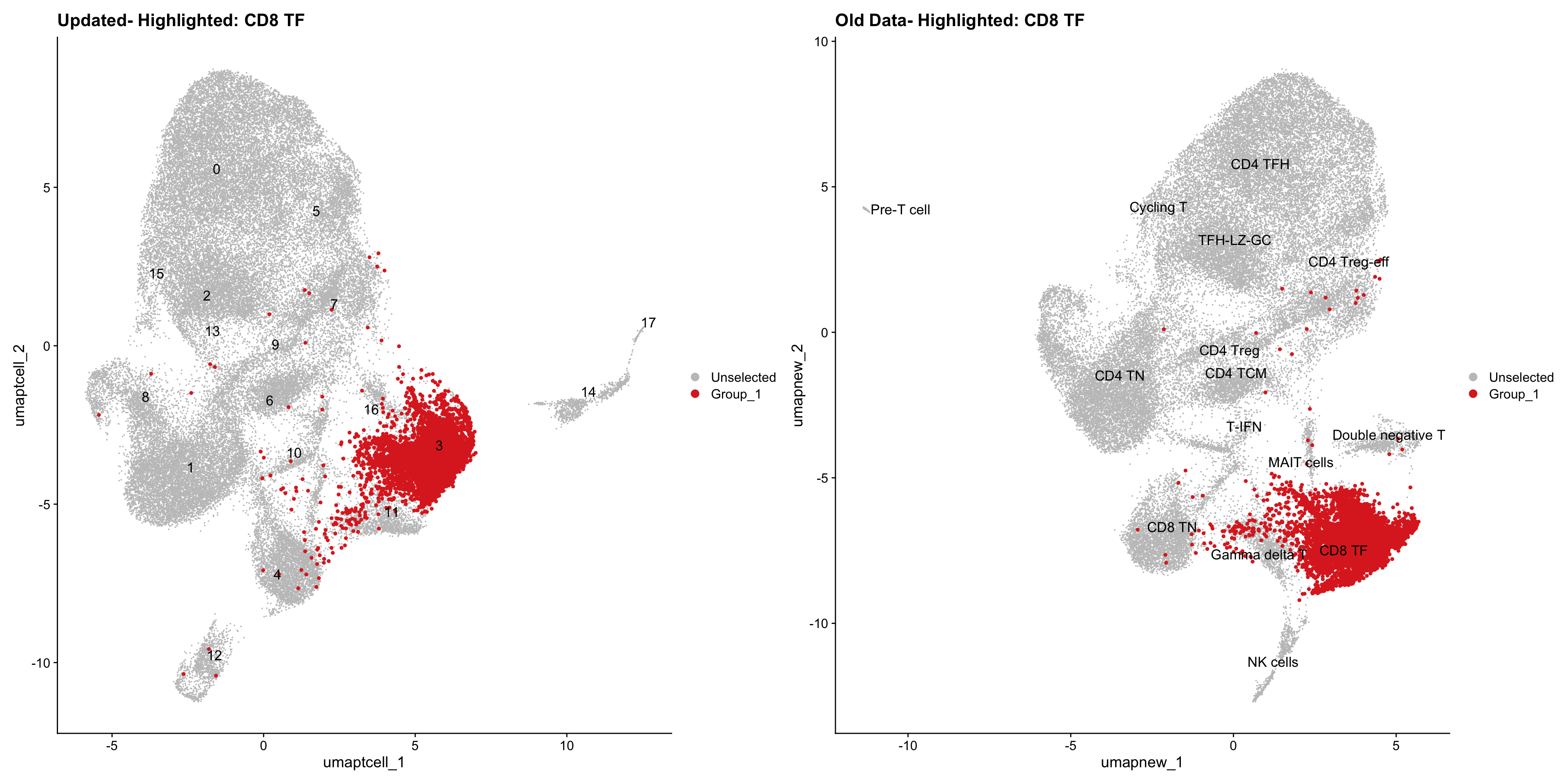
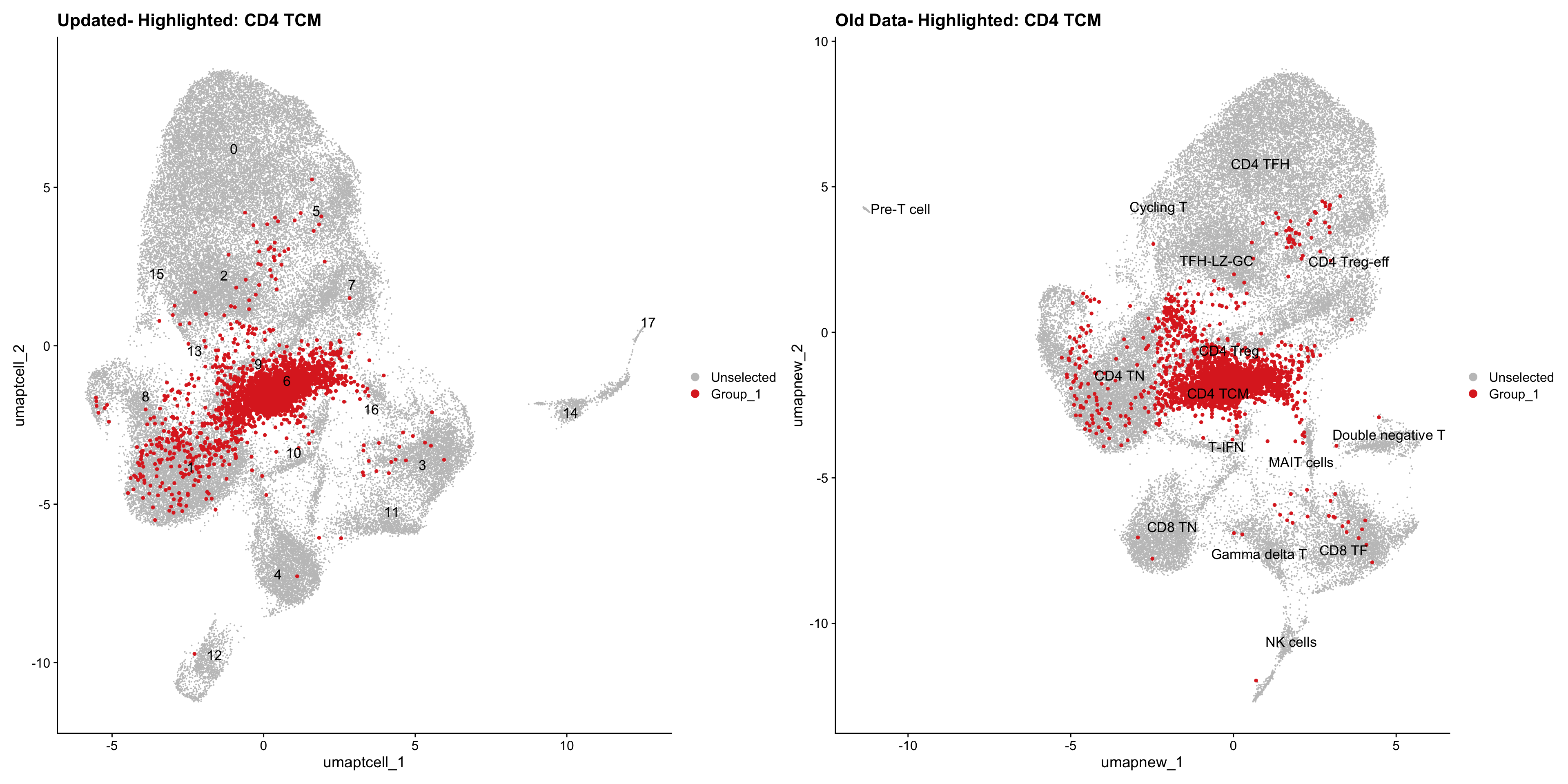
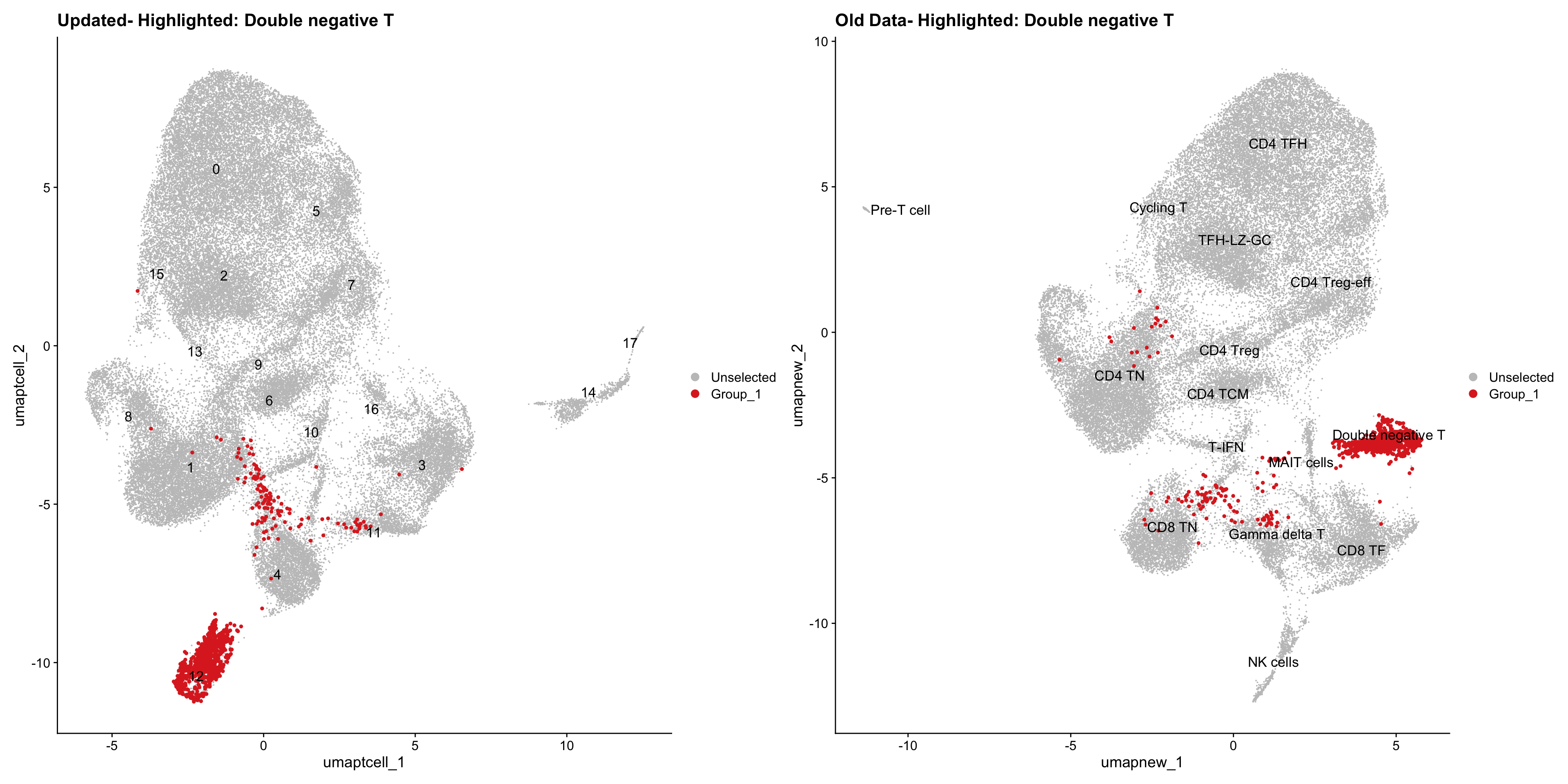
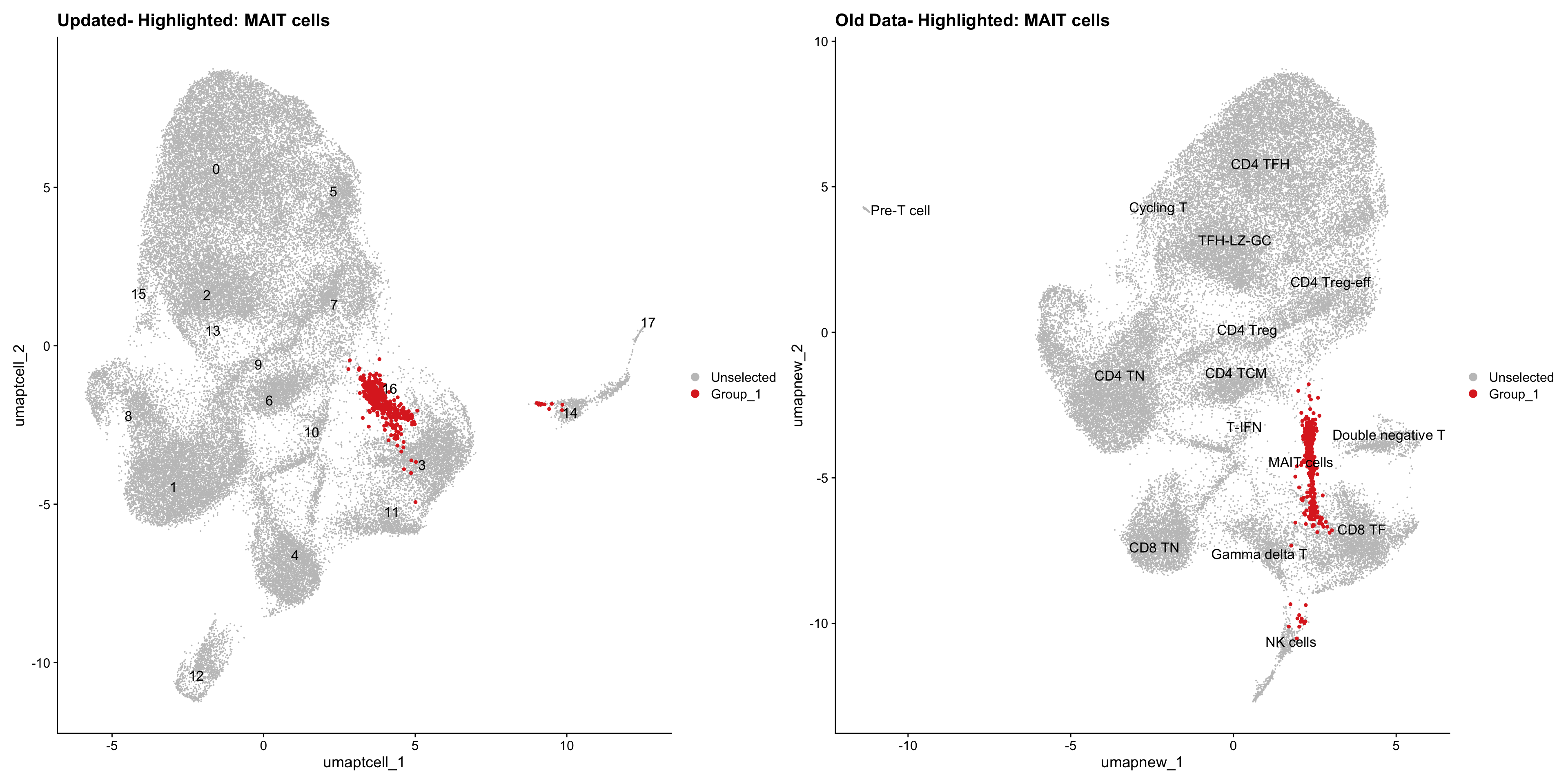
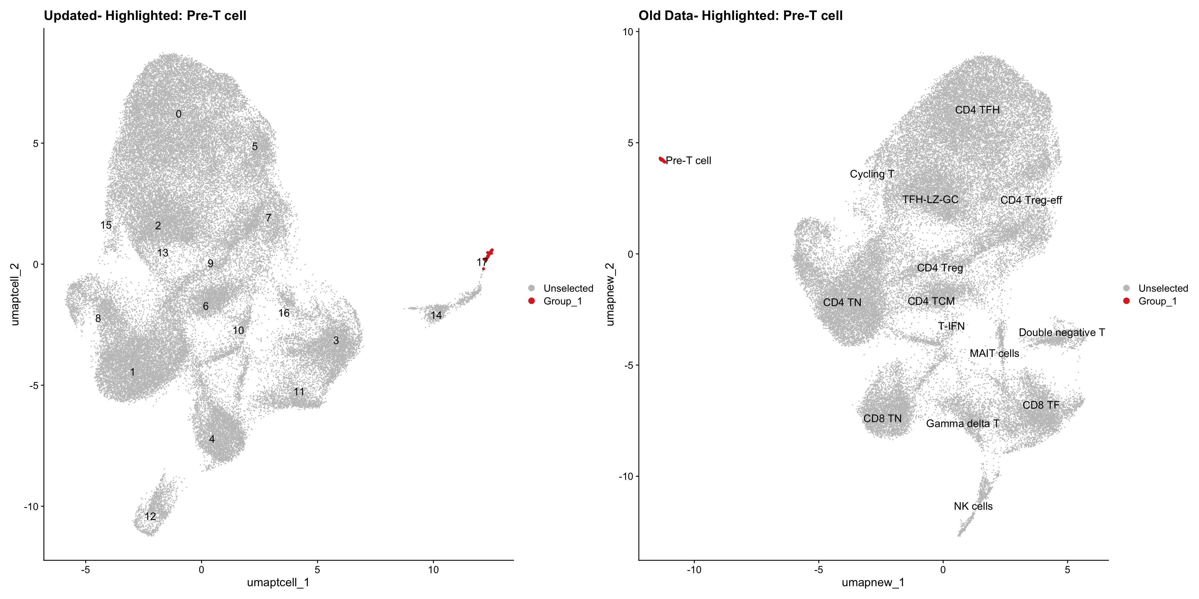
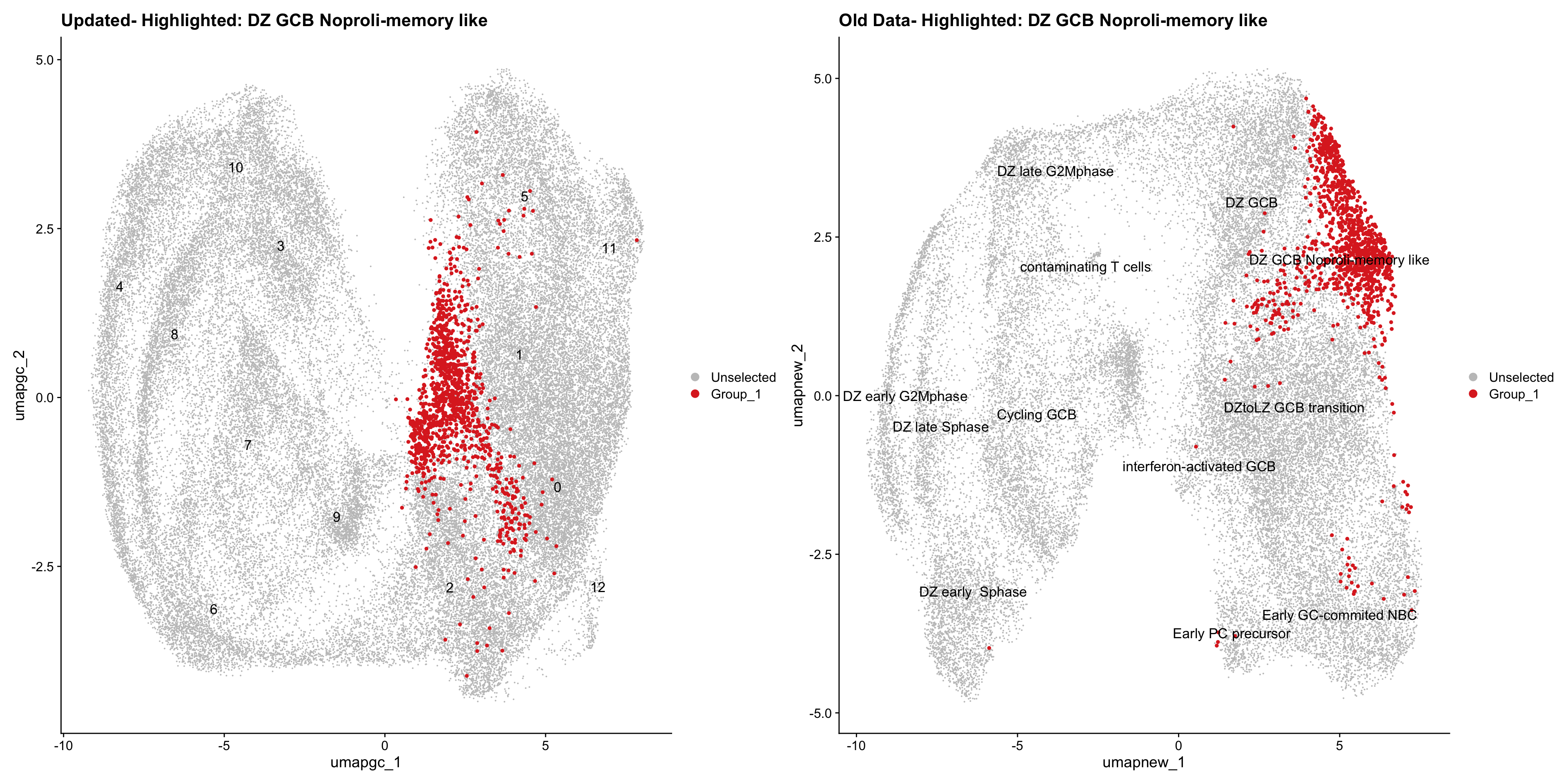
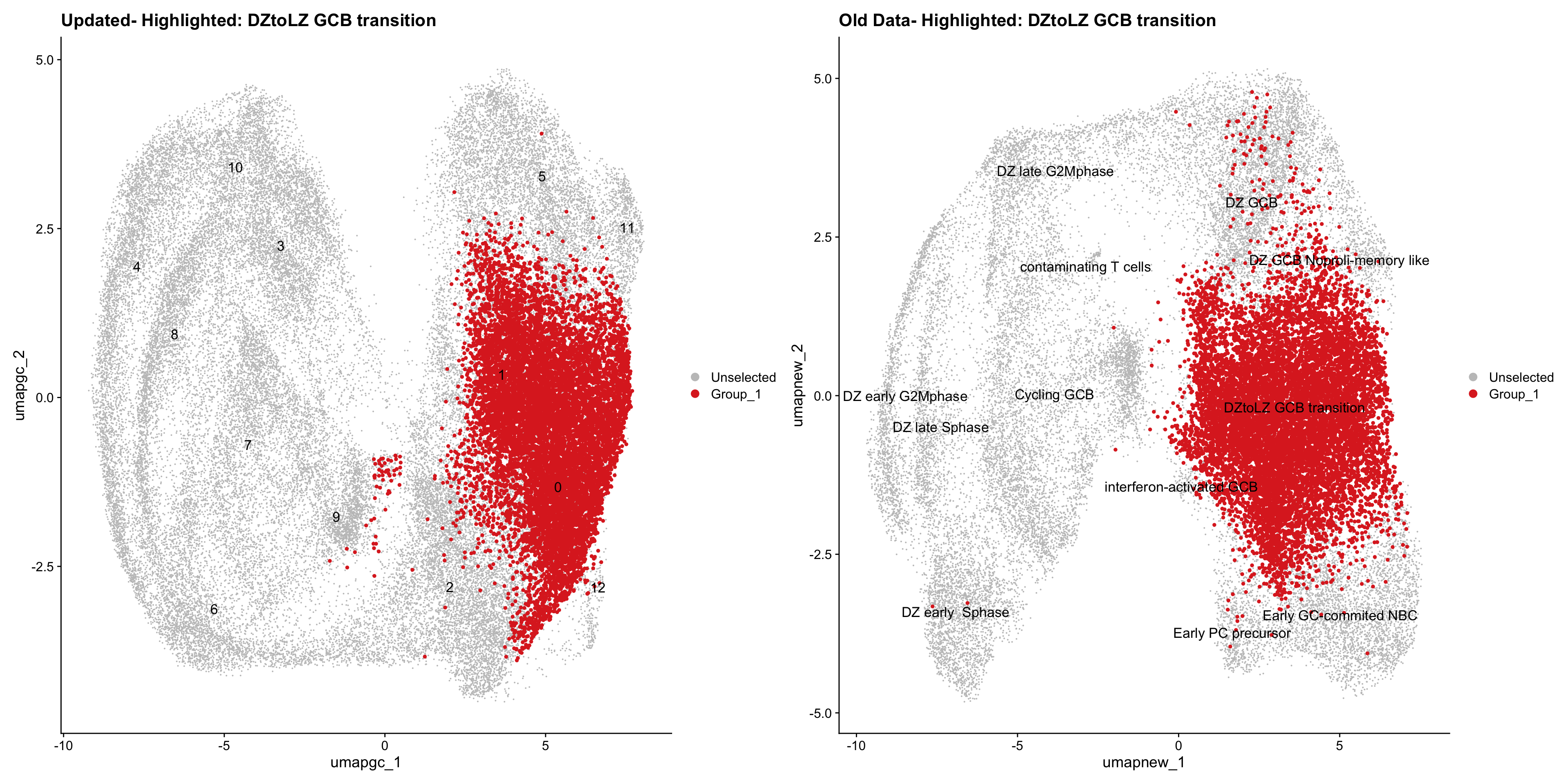
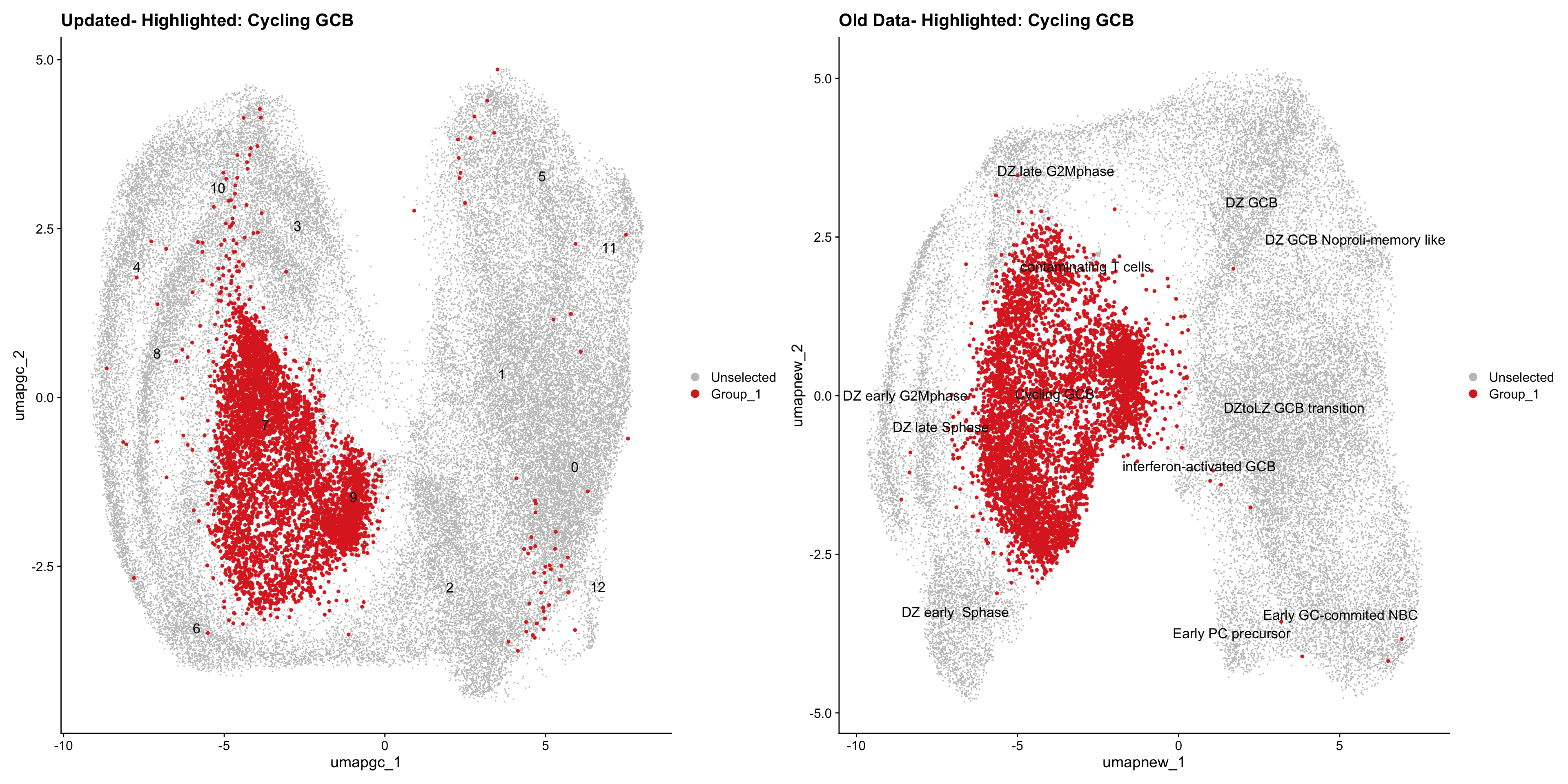
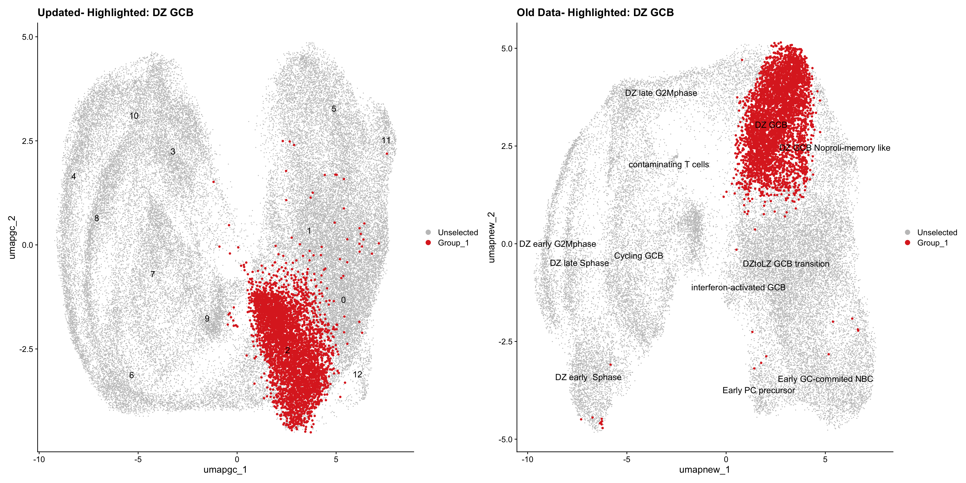
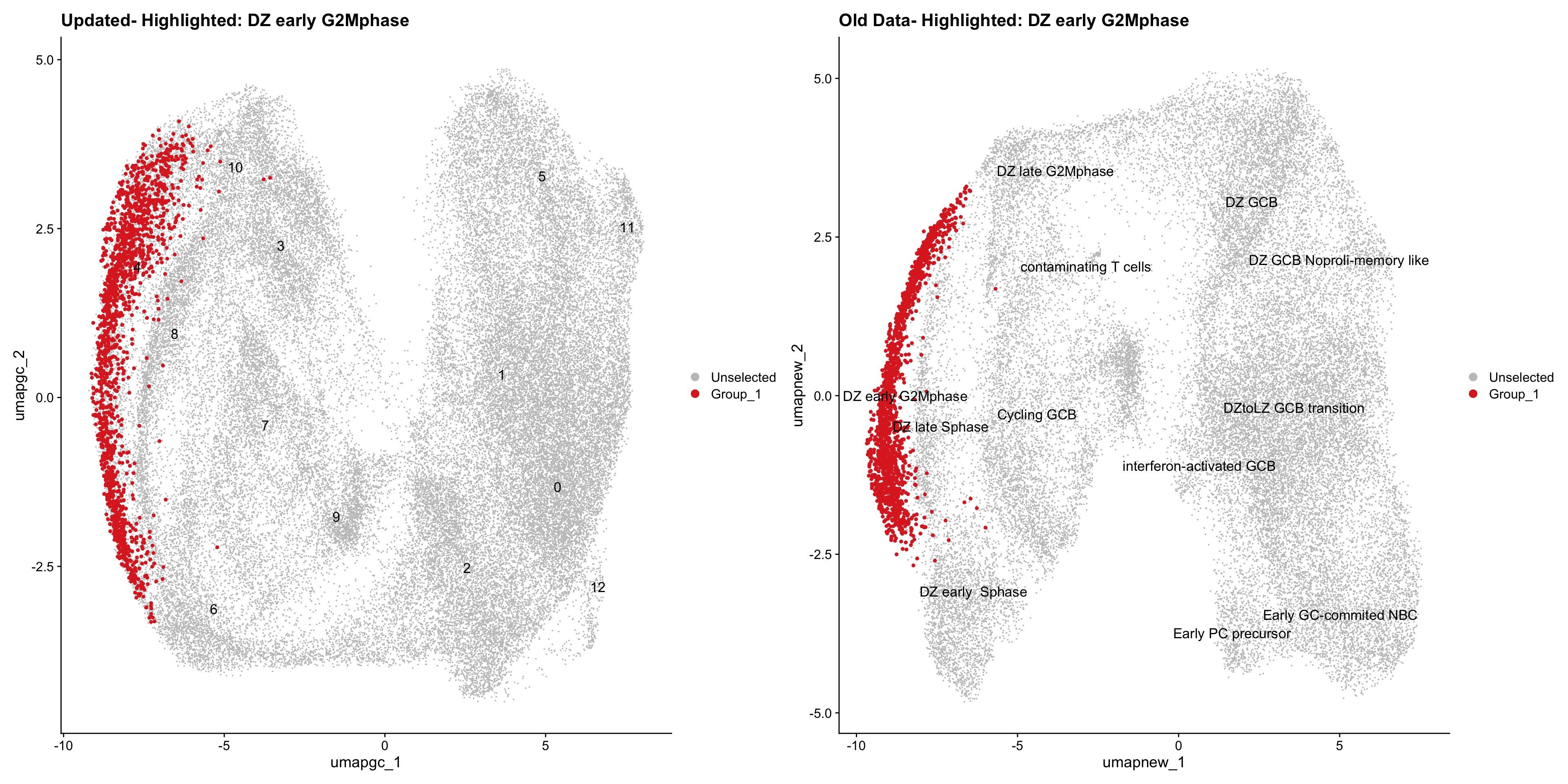
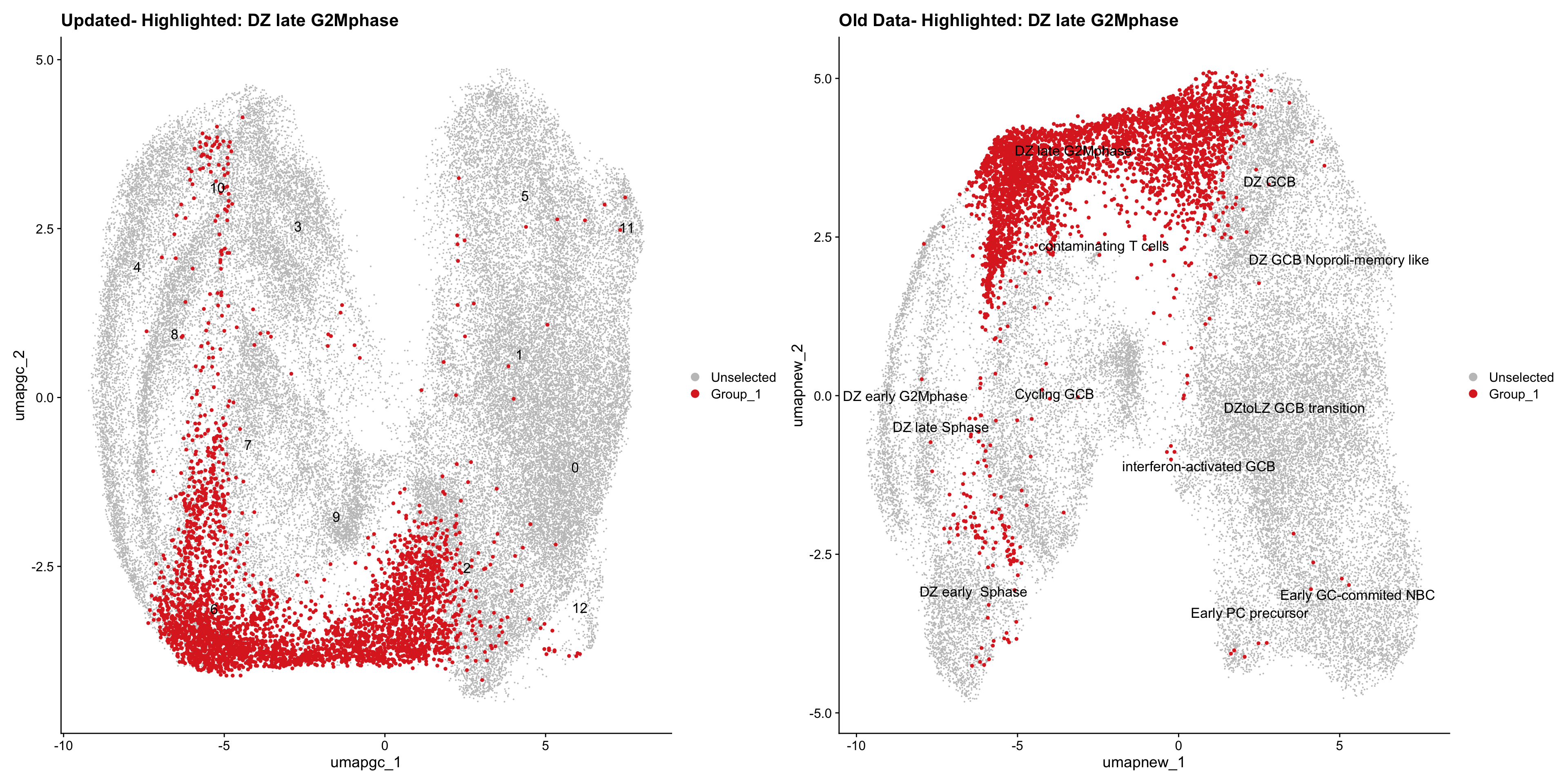
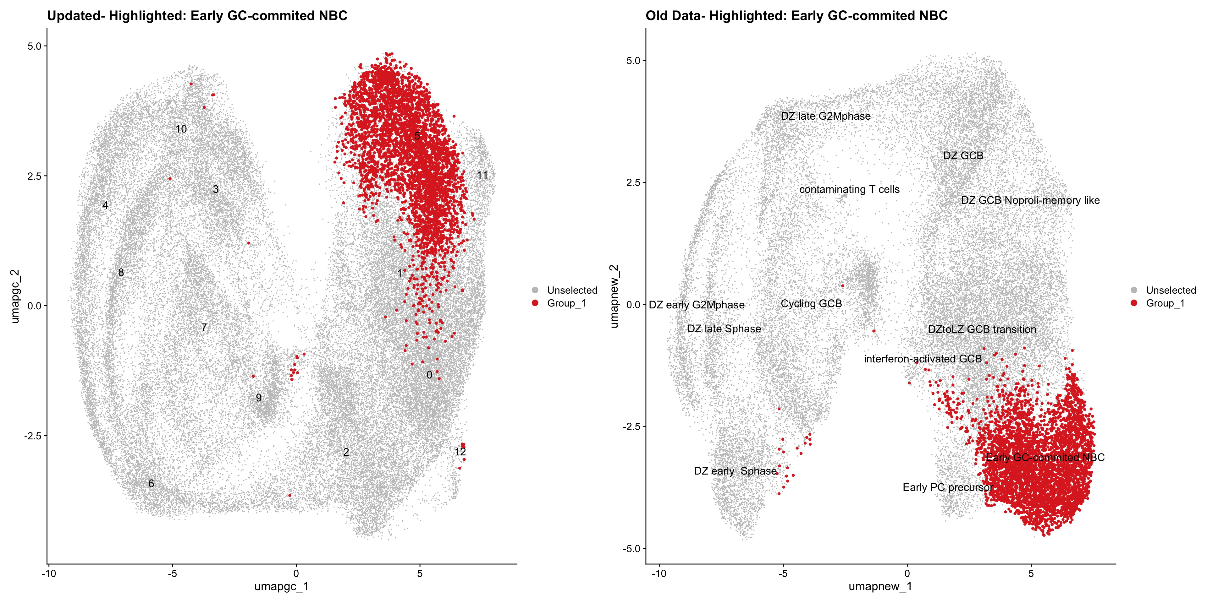
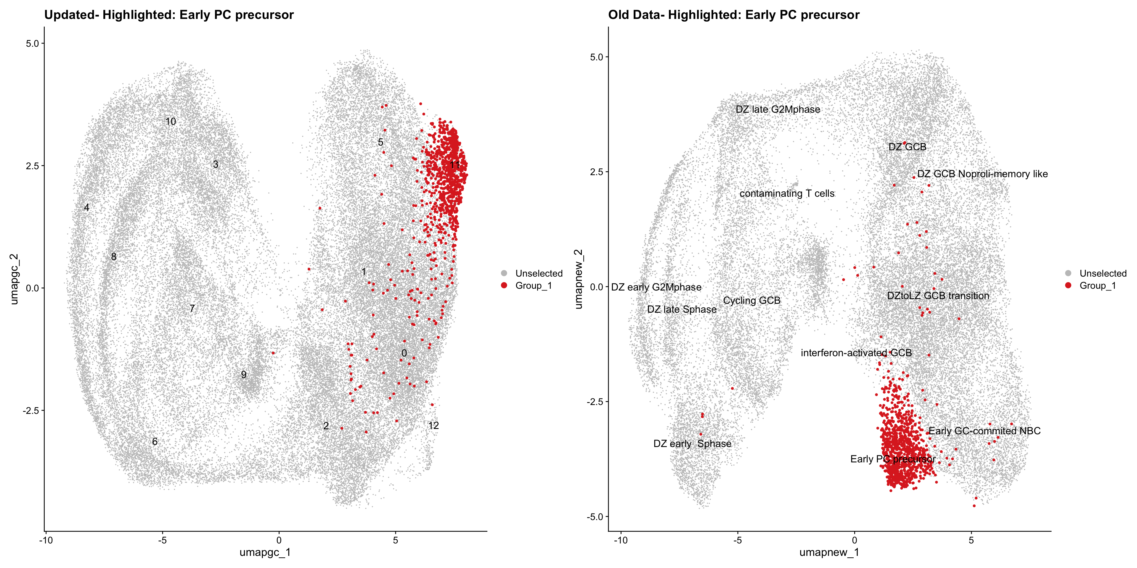
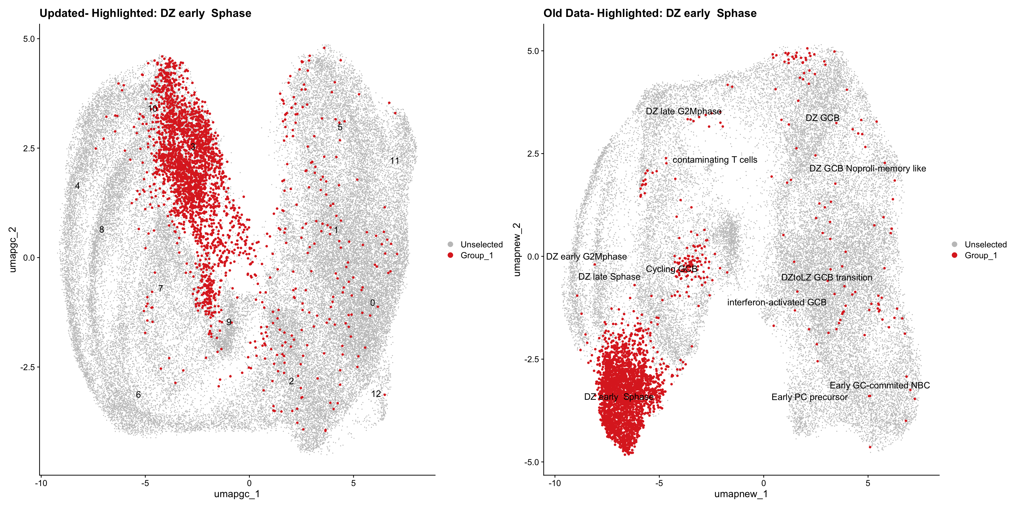
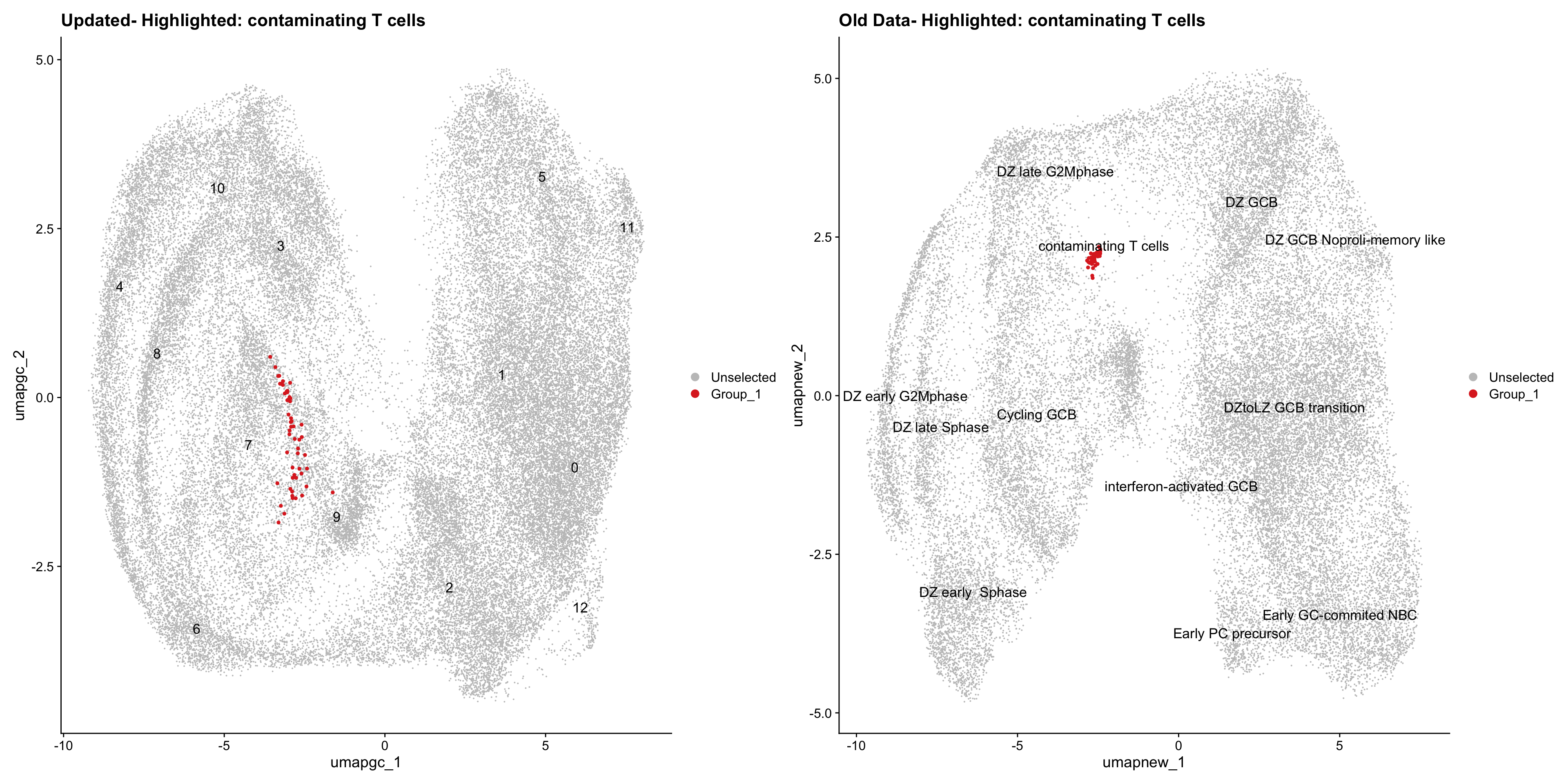
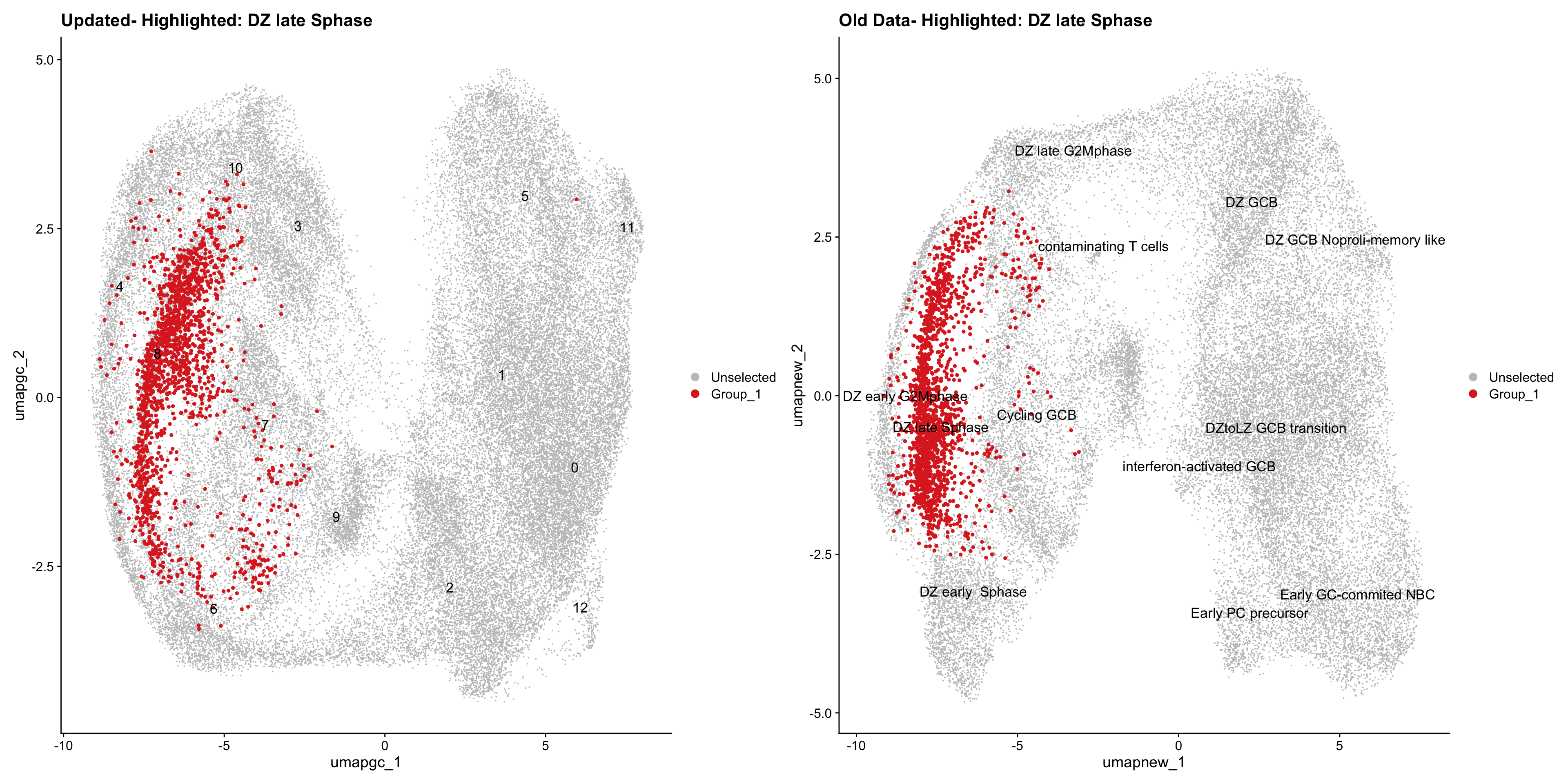
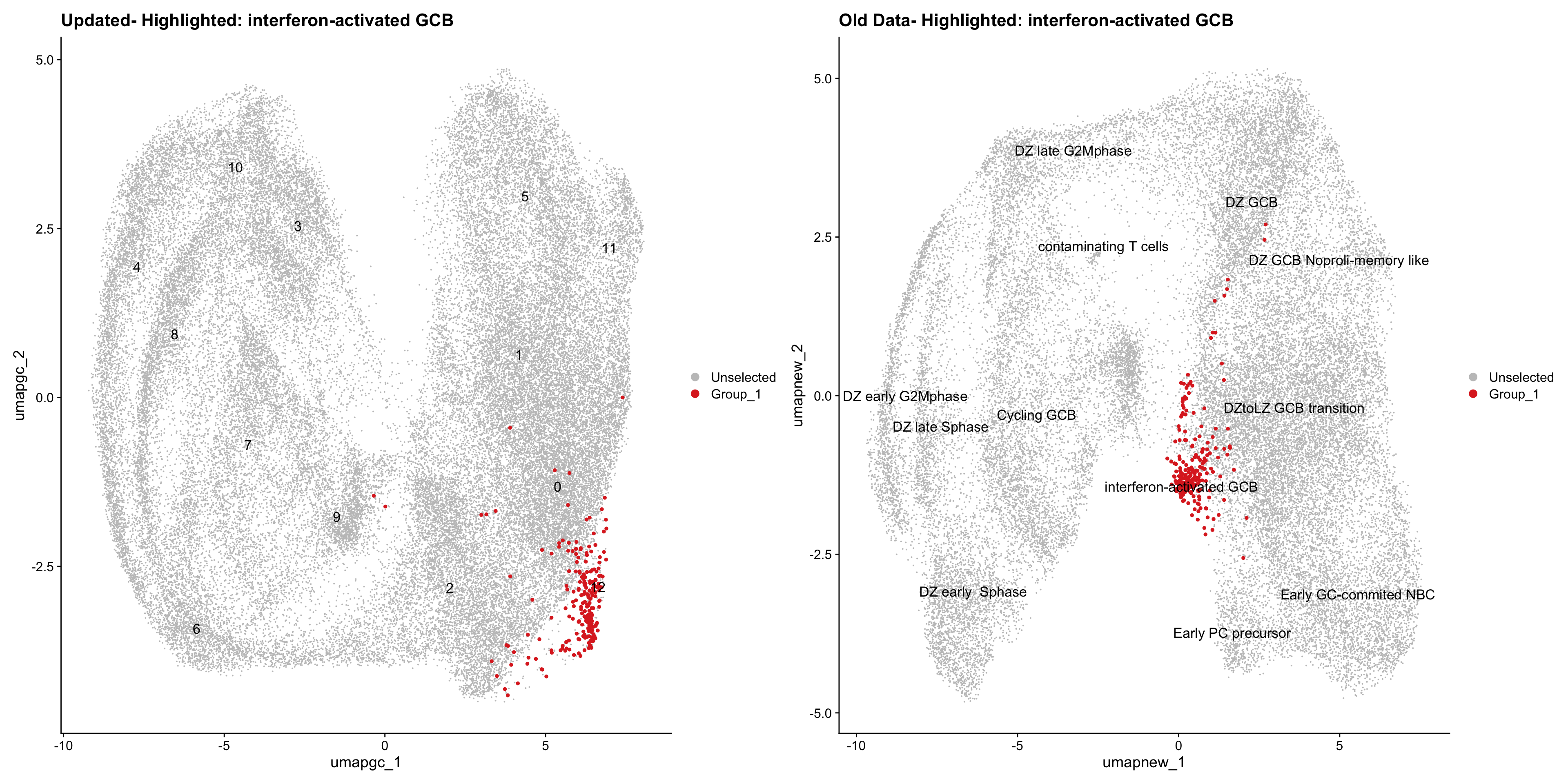
old_obj <- readRDS(out1)cell_types <- unique(old_obj$cell_labels)
for (cell_type in cell_types) {
cl_cells <- WhichCells(old_obj, idents = cell_type)
p <- DimPlot(
merged_obj,
reduction = "umap.harmony",
label = TRUE,
label.size = 4.5,
repel = TRUE,
raster = FALSE,
cells.highlight = cl_cells
) +
ggtitle(paste("Updated- Highlighted:", cell_type))
p1 <- DimPlot(
old_obj,
reduction = "umap.harmony",
label = T,
label.size = 4.5,
repel = TRUE,
raster = FALSE,
cells.highlight = cl_cells
) +
ggtitle(paste("Old Data- Highlighted:", cell_type))
print(p | p1)
}
| Version | Author | Date |
|---|---|---|
| 4cbf4d0 | Gunjan Dixit | 2024-12-17 |
| Version | Author | Date |
|---|---|---|
| 4cbf4d0 | Gunjan Dixit | 2024-12-17 |
| Version | Author | Date |
|---|---|---|
| 4cbf4d0 | Gunjan Dixit | 2024-12-17 |
| Version | Author | Date |
|---|---|---|
| 4cbf4d0 | Gunjan Dixit | 2024-12-17 |
| Version | Author | Date |
|---|---|---|
| 4cbf4d0 | Gunjan Dixit | 2024-12-17 |
| Version | Author | Date |
|---|---|---|
| 4cbf4d0 | Gunjan Dixit | 2024-12-17 |
| Version | Author | Date |
|---|---|---|
| 4cbf4d0 | Gunjan Dixit | 2024-12-17 |
| Version | Author | Date |
|---|---|---|
| 4cbf4d0 | Gunjan Dixit | 2024-12-17 |
| Version | Author | Date |
|---|---|---|
| 4cbf4d0 | Gunjan Dixit | 2024-12-17 |
| Version | Author | Date |
|---|---|---|
| 4cbf4d0 | Gunjan Dixit | 2024-12-17 |
| Version | Author | Date |
|---|---|---|
| 4cbf4d0 | Gunjan Dixit | 2024-12-17 |
| Version | Author | Date |
|---|---|---|
| 4cbf4d0 | Gunjan Dixit | 2024-12-17 |
| Version | Author | Date |
|---|---|---|
| 4cbf4d0 | Gunjan Dixit | 2024-12-17 |
| Version | Author | Date |
|---|---|---|
| 4cbf4d0 | Gunjan Dixit | 2024-12-17 |
| Version | Author | Date |
|---|---|---|
| 4cbf4d0 | Gunjan Dixit | 2024-12-17 |
| Version | Author | Date |
|---|---|---|
| 4cbf4d0 | Gunjan Dixit | 2024-12-17 |
| Version | Author | Date |
|---|---|---|
| 4cbf4d0 | Gunjan Dixit | 2024-12-17 |
| Version | Author | Date |
|---|---|---|
| 4cbf4d0 | Gunjan Dixit | 2024-12-17 |
| Version | Author | Date |
|---|---|---|
| 4cbf4d0 | Gunjan Dixit | 2024-12-17 |
| Version | Author | Date |
|---|---|---|
| 4cbf4d0 | Gunjan Dixit | 2024-12-17 |
| Version | Author | Date |
|---|---|---|
| 4cbf4d0 | Gunjan Dixit | 2024-12-17 |
| Version | Author | Date |
|---|---|---|
| 4cbf4d0 | Gunjan Dixit | 2024-12-17 |
| Version | Author | Date |
|---|---|---|
| 4cbf4d0 | Gunjan Dixit | 2024-12-17 |
| Version | Author | Date |
|---|---|---|
| 4cbf4d0 | Gunjan Dixit | 2024-12-17 |
Updated cell-type labels (all clusters)
cell_labels <- readxl::read_excel(here("data/cell_labels_Mel_v4_Dec2024/earlyAIR_Tonsils_all.xlsx"), sheet = "all_clusters")

new_cluster_names <- cell_labels %>%
  dplyr::select(cluster, annotation) %>%
  deframe()

merged_obj <- RenameIdents(merged_obj, new_cluster_names)
merged_obj@meta.data$cell_labels <- Idents(merged_obj)

p3 <- DimPlot(merged_obj, reduction = "umap.harmony", raster = FALSE, repel = TRUE, label = TRUE, label.size = 3.5) + ggtitle(paste0(tissue, ": UMAP with Updated cell types"))

p3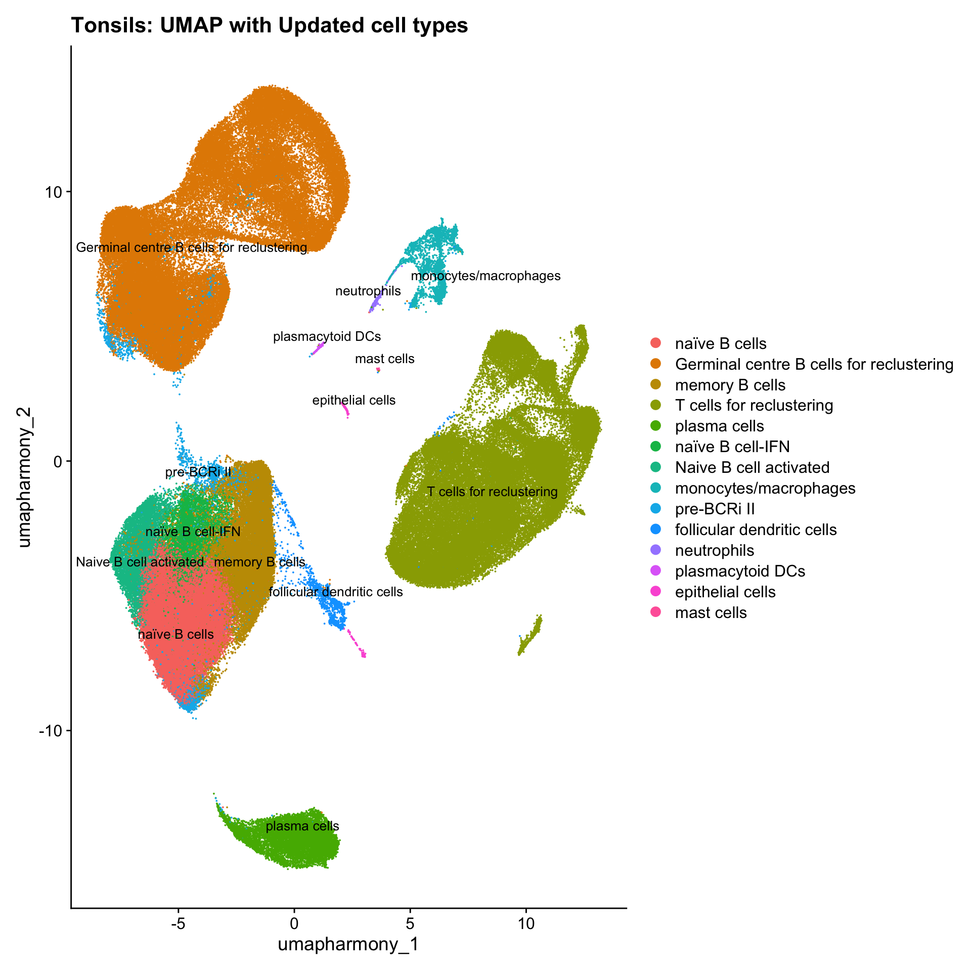
| Version | Author | Date |
|---|---|---|
| 54e4ec2 | Gunjan Dixit | 2025-01-08 |
Summary plots
palette1 <- paletteer::paletteer_d("ggthemes::Classic_20")
palette2 <- paletteer::paletteer_d("Polychrome::light")
combined_palette <- unique(c(palette1, palette2))

labels <- c("cell_labels")

p <- vector("list",length(labels))
for(label in labels){
  merged_obj@meta.data %>%
    ggplot(aes(x = !!sym(label),
               fill = !!sym(label))) +
    geom_bar() +
    geom_text(aes(label = ..count..), stat = "count",
              vjust = -0.5, colour = "black", size = 2) +
    scale_y_log10() +
    theme(axis.text.x = element_blank(),
          axis.title.x = element_blank(),
          axis.ticks.x = element_blank()) +
    NoLegend() +
    labs(y = "No. Cells (log scale)") -> p1

  merged_obj@meta.data %>%
    dplyr::select(!!sym(label), donor_id) %>%
    group_by(!!sym(label), donor_id) %>%
    summarise(num = n()) %>%
    mutate(prop = num / sum(num)) %>%
  ggplot(aes(x = !!sym(label), y = prop * 100,
             fill = donor_id)) +
    geom_bar(stat = "identity") +
    theme(axis.text.x = element_text(angle = 90,
                                     vjust = 0.5,
                                     hjust = 1,
                                     size = 8)) +
    labs(y = "% Cells", fill = "Donor") +
  scale_fill_manual(values = combined_palette) -> p2

  (p1 / p2) & theme(legend.text = element_text(size = 8),
                  legend.key.size = unit(3, "mm")) -> p[[label]]
}
`summarise()` has grouped output by 'cell_labels'. You can override using the
`.groups` argument.p[[1]]
NULL
$cell_labels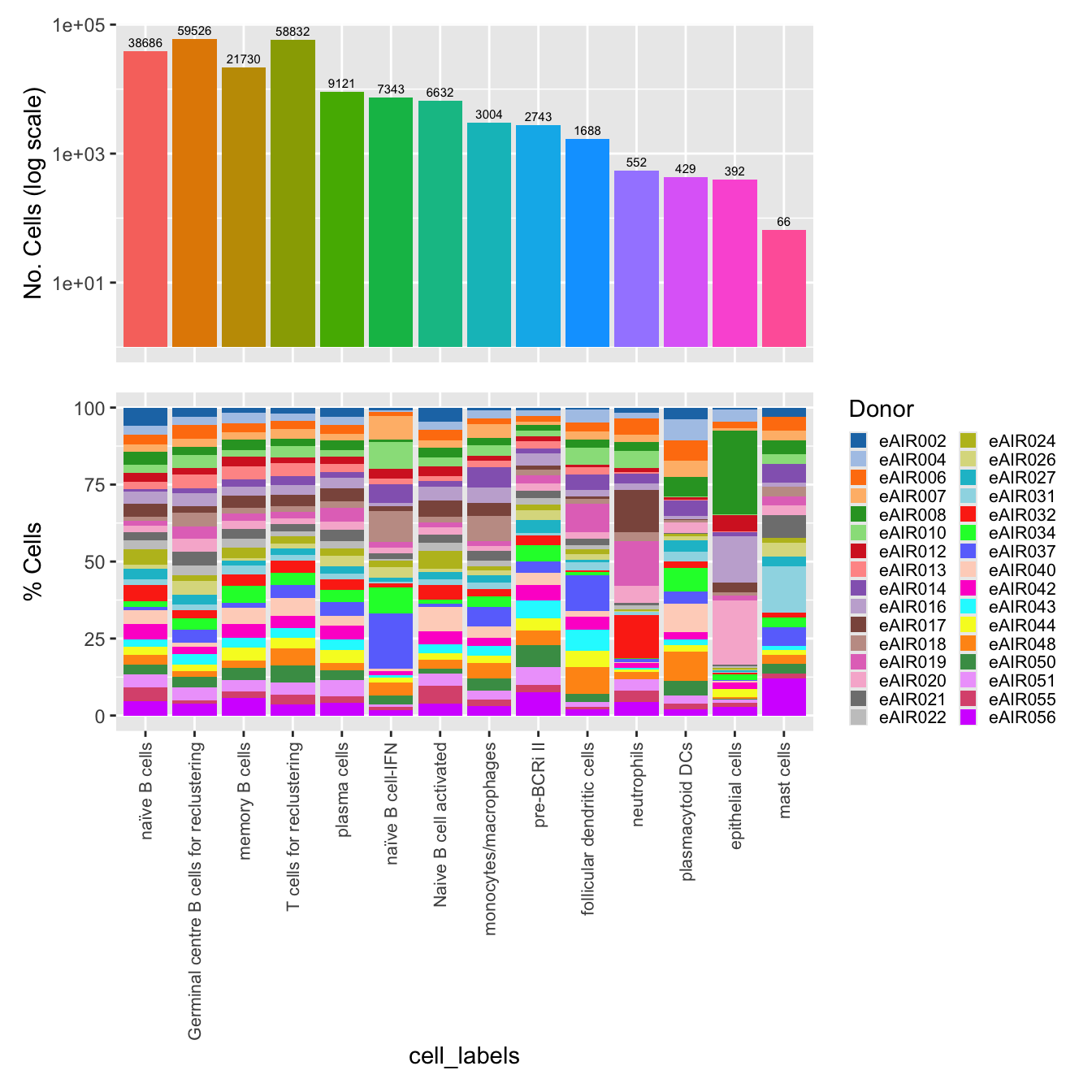
| Version | Author | Date |
|---|---|---|
| 54e4ec2 | Gunjan Dixit | 2025-01-08 |
Reclustering T cell subtypes
Reclustering clusters
The marker genes for this reclustering can be found here-
Tonsils_Tcell_population_res.0.5
#sub_clusters <- c(3, 4, 5, 11,15,17, 21, 22, 23)
#idx <- which(merged_obj$cluster %in% sub_clusters)
idx <- which(Idents(merged_obj) %in% "T cells for reclustering")
paed_sub <- merged_obj[,idx]
paed_sub
An object of class Seurat
17566 features across 58832 samples within 1 assay
Active assay: RNA (17566 features, 2000 variable features)
3 layers present: data, counts, scale.data
4 dimensional reductions calculated: pca, umap.unintegrated, harmony, umap.harmony# Visualize the clustering results
DimPlot(paed_sub, reduction = "umap.harmony", group.by = "cluster", label = TRUE, label.size = 2.5, repel = TRUE, raster = FALSE )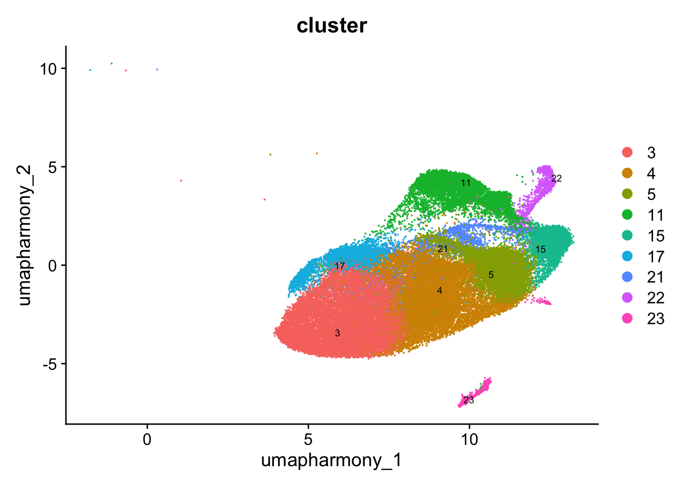
| Version | Author | Date |
|---|---|---|
| 4cbf4d0 | Gunjan Dixit | 2024-12-17 |
paed_sub <- paed_sub %>%
  NormalizeData() %>%
  FindVariableFeatures() %>%
  ScaleData() %>%
  RunPCA()

paed_sub <- RunUMAP(paed_sub, dims = 1:30, reduction = "pca", reduction.name = "umap.tcell")
meta_data_columns <- colnames(paed_sub@meta.data)
columns_to_remove <- grep("^RNA_snn_res", meta_data_columns, value = TRUE)
paed_sub@meta.data <- paed_sub@meta.data[, !(colnames(paed_sub@meta.data) %in% columns_to_remove)]resolutions <- seq(0.1, 1, by = 0.1)
paed_sub <- FindNeighbors(paed_sub, dims = 1:30, reduction = "pca")
paed_sub <- FindClusters(paed_sub, resolution = resolutions )Modularity Optimizer version 1.3.0 by Ludo Waltman and Nees Jan van Eck
Number of nodes: 58832
Number of edges: 1758188
Running Louvain algorithm...
Maximum modularity in 10 random starts: 0.9519
Number of communities: 6
Elapsed time: 13 seconds
Modularity Optimizer version 1.3.0 by Ludo Waltman and Nees Jan van Eck
Number of nodes: 58832
Number of edges: 1758188
Running Louvain algorithm...
Maximum modularity in 10 random starts: 0.9323
Number of communities: 10
Elapsed time: 10 seconds
Modularity Optimizer version 1.3.0 by Ludo Waltman and Nees Jan van Eck
Number of nodes: 58832
Number of edges: 1758188
Running Louvain algorithm...
Maximum modularity in 10 random starts: 0.9188
Number of communities: 14
Elapsed time: 10 seconds
Modularity Optimizer version 1.3.0 by Ludo Waltman and Nees Jan van Eck
Number of nodes: 58832
Number of edges: 1758188
Running Louvain algorithm...
Maximum modularity in 10 random starts: 0.9080
Number of communities: 16
Elapsed time: 10 seconds
Modularity Optimizer version 1.3.0 by Ludo Waltman and Nees Jan van Eck
Number of nodes: 58832
Number of edges: 1758188
Running Louvain algorithm...
Maximum modularity in 10 random starts: 0.8984
Number of communities: 18
Elapsed time: 9 seconds
Modularity Optimizer version 1.3.0 by Ludo Waltman and Nees Jan van Eck
Number of nodes: 58832
Number of edges: 1758188
Running Louvain algorithm...
Maximum modularity in 10 random starts: 0.8910
Number of communities: 19
Elapsed time: 10 seconds
Modularity Optimizer version 1.3.0 by Ludo Waltman and Nees Jan van Eck
Number of nodes: 58832
Number of edges: 1758188
Running Louvain algorithm...
Maximum modularity in 10 random starts: 0.8838
Number of communities: 20
Elapsed time: 8 seconds
Modularity Optimizer version 1.3.0 by Ludo Waltman and Nees Jan van Eck
Number of nodes: 58832
Number of edges: 1758188
Running Louvain algorithm...
Maximum modularity in 10 random starts: 0.8762
Number of communities: 22
Elapsed time: 9 seconds
Modularity Optimizer version 1.3.0 by Ludo Waltman and Nees Jan van Eck
Number of nodes: 58832
Number of edges: 1758188
Running Louvain algorithm...
Maximum modularity in 10 random starts: 0.8693
Number of communities: 22
Elapsed time: 10 seconds
Modularity Optimizer version 1.3.0 by Ludo Waltman and Nees Jan van Eck
Number of nodes: 58832
Number of edges: 1758188
Running Louvain algorithm...
Maximum modularity in 10 random starts: 0.8632
Number of communities: 24
Elapsed time: 8 secondsclustree(paed_sub, prefix = "RNA_snn_res.")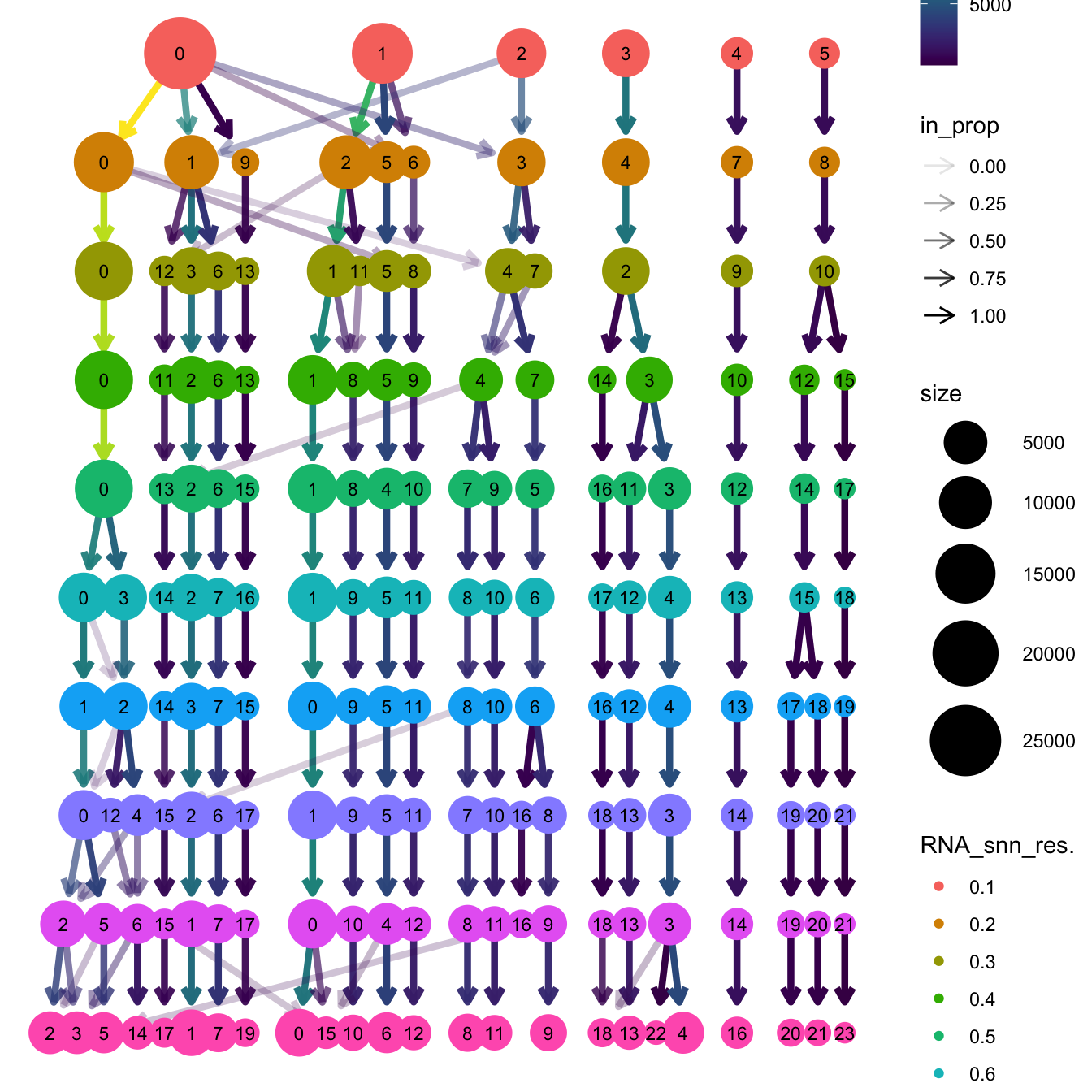
| Version | Author | Date |
|---|---|---|
| 4cbf4d0 | Gunjan Dixit | 2024-12-17 |
# Visualize the clustering results
DimPlot(paed_sub, group.by = "RNA_snn_res.0.5", reduction = "umap.tcell", label = TRUE, label.size = 2.5, repel = TRUE, raster = FALSE )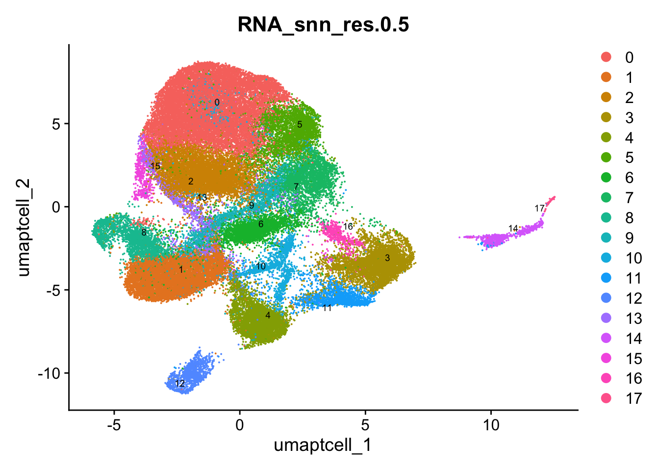
opt_res <- "RNA_snn_res.0.5"
n <- nlevels(paed_sub$RNA_snn_res.0.5)
paed_sub$RNA_snn_res.0.5 <- factor(paed_sub$RNA_snn_res.0.5, levels = seq(0,n-1))
paed_sub$seurat_clusters <- NULL
paed_sub$cluster <- paed_sub$RNA_snn_res.0.5
Idents(paed_sub) <- paed_sub$cluster
paed_sub.markers <- FindAllMarkers(paed_sub, only.pos = TRUE, min.pct = 0.25, logfc.threshold = 0.25)Calculating cluster 0Calculating cluster 1Calculating cluster 2Calculating cluster 3Calculating cluster 4Calculating cluster 5Calculating cluster 6Calculating cluster 7Calculating cluster 8Calculating cluster 9Calculating cluster 10Calculating cluster 11Calculating cluster 12Calculating cluster 13Calculating cluster 14Calculating cluster 15Calculating cluster 16Calculating cluster 17paed_sub.markers %>%
group_by(cluster) %>% unique() %>%
top_n(n = 5, wt = avg_log2FC) -> top5
paed_sub.markers %>%
group_by(cluster) %>%
slice_head(n=1) %>%
pull(gene) -> best.wilcox.gene.per.cluster
best.wilcox.gene.per.cluster [1] "TOX2" "KLF2" "GPR183" "CCL5" "CD8A" "CTLA4" "KLF2" "COL5A3"
[9] "LEF1" "FOXP3" "IFI44L" "KLRK1" "GZMK" "ZAP70" "TRDC" "ACTB"
[17] "NKG7" "ARPP21"Violin plot shows the expression of top marker gene per cluster.
VlnPlot(paed_sub, features=best.wilcox.gene.per.cluster, ncol = 2, raster = FALSE, pt.size = FALSE)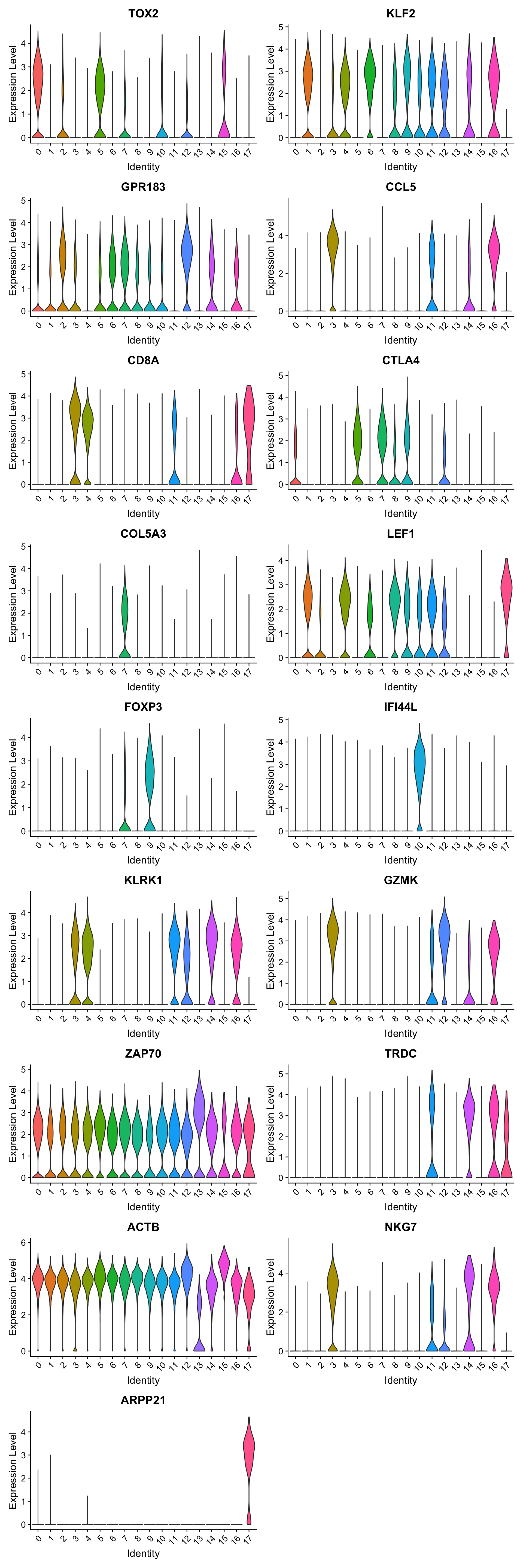
| Version | Author | Date |
|---|---|---|
| 4cbf4d0 | Gunjan Dixit | 2024-12-17 |
Feature plot shows the expression of top marker genes per cluster.
FeaturePlot(paed_sub,features=best.wilcox.gene.per.cluster, reduction = 'umap.tcell', raster = FALSE, ncol = 3, label = TRUE)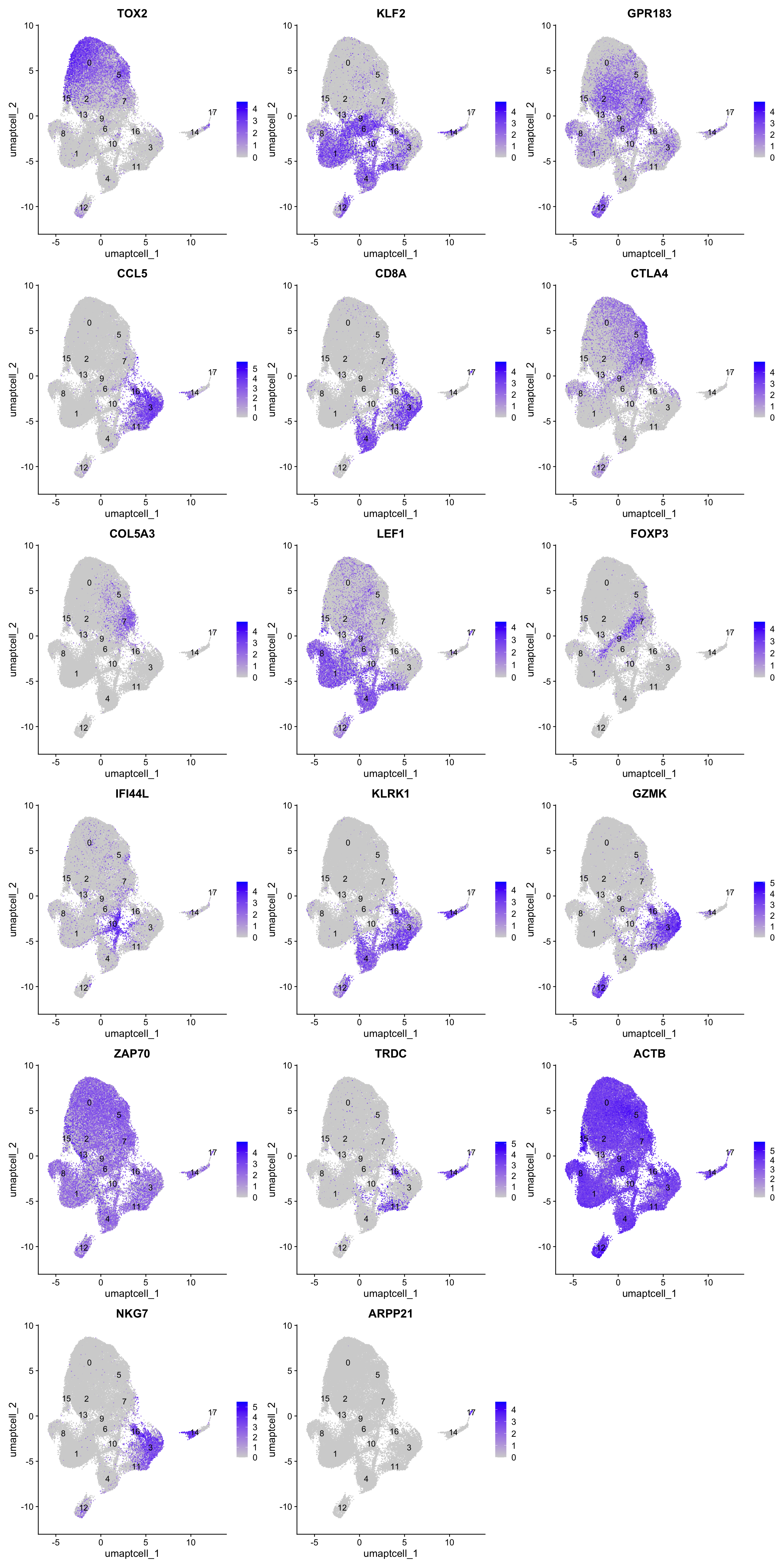
Top 10 marker genes from Seurat
## Seurat top markers
top10 <- paed_sub.markers %>%
    group_by(cluster) %>%
    top_n(n = 10, wt = avg_log2FC) %>%
    ungroup() %>%
    distinct(gene, .keep_all = TRUE) %>%
    arrange(cluster, desc(avg_log2FC))

cluster_colors <- paletteer::paletteer_d("pals::glasbey")[factor(top10$cluster)]

DotPlot(paed_sub,
        features = unique(top10$gene),
        group.by = opt_res,
        cols = c("azure1", "blueviolet"),
        dot.scale = 3, assay = "RNA") +
    RotatedAxis() +
    FontSize(y.text = 8, x.text = 12) +
    labs(y = element_blank(), x = element_blank()) +
    coord_flip() +
    theme(axis.text.y = element_text(color = cluster_colors)) +
    ggtitle("Top 10 marker genes per cluster (Seurat)")
Warning: Vectorized input to `element_text()` is not officially supported.
ℹ Results may be unexpected or may change in future versions of ggplot2.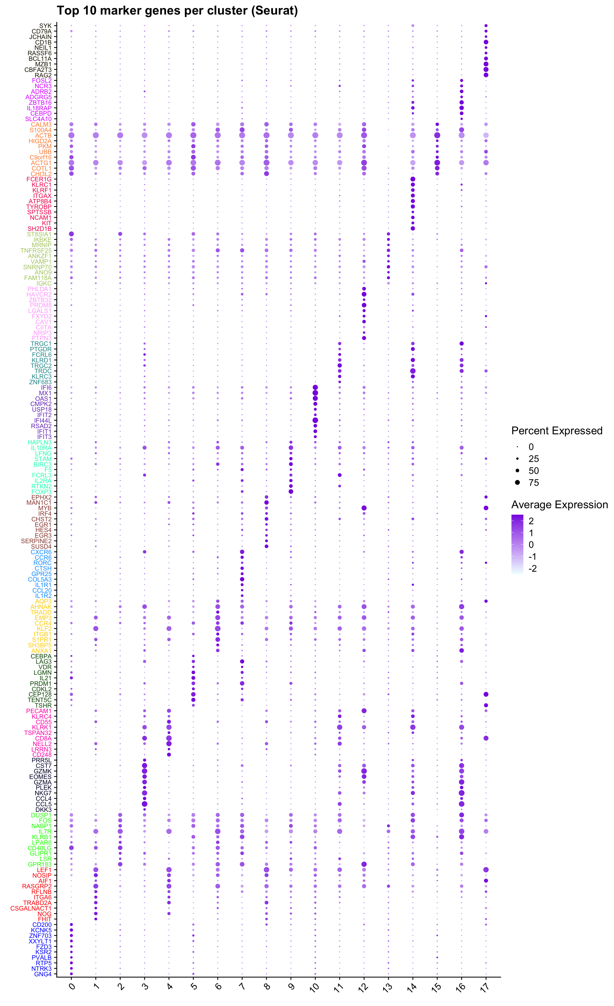
| Version | Author | Date |
|---|---|---|
| 54e4ec2 | Gunjan Dixit | 2025-01-08 |
palette1 <- paletteer::paletteer_d("ggthemes::Classic_20")
palette2 <- paletteer::paletteer_d("Polychrome::light")
combined_palette <- unique(c(palette1, palette2))

labels <- "RNA_snn_res.0.5"

p <- vector("list",length(labels))
for(label in labels){
  paed_sub@meta.data %>%
    ggplot(aes(x = !!sym(label),
               fill = !!sym(label))) +
    geom_bar() +
    geom_text(aes(label = ..count..), stat = "count",
              vjust = -0.5, colour = "black", size = 2) +
    scale_y_log10() +
    theme(axis.text.x = element_blank(),
          axis.title.x = element_blank(),
          axis.ticks.x = element_blank()) +
    NoLegend() +
    labs(y = "No. Cells (log scale)") -> p1

  paed_sub@meta.data %>%
    dplyr::select(!!sym(label), donor_id) %>%
    group_by(!!sym(label), donor_id) %>%
    summarise(num = n()) %>%
    mutate(prop = num / sum(num)) %>%
  ggplot(aes(x = !!sym(label), y = prop * 100,
             fill = donor_id)) +
    geom_bar(stat = "identity") +
    theme(axis.text.x = element_text(angle = 90,
                                     vjust = 0.5,
                                     hjust = 1,
                                     size = 8)) +
    labs(y = "% Cells", fill = "Donor") +
  scale_fill_manual(values = combined_palette) -> p2

  (p1 / p2) & theme(legend.text = element_text(size = 8),
                  legend.key.size = unit(3, "mm")) -> p[[label]]
}
`summarise()` has grouped output by 'RNA_snn_res.0.5'. You can override using
the `.groups` argument.p[[1]]
NULL
$RNA_snn_res.0.5
out_markers <- here("output",
            "CSV_v2", tissue,
            paste(tissue,"_Marker_genes_Reclustered_Tcell_population.",opt_res, sep = ""))

dir.create(out_markers, recursive = TRUE, showWarnings = FALSE)

for (cl in unique(paed_sub.markers$cluster)) {
  cluster_data <- paed_sub.markers %>% dplyr::filter(cluster == cl)
  file_name <- here(out_markers, paste0("G000231_Neeland_",tissue, "_cluster_", cl, ".csv"))
  if (!file.exists(file_name)) {
  write.csv(cluster_data, file = file_name)
  }
}
Corresponding Azimuth labels (T cell subsets)
## Level 1
DimPlot(paed_sub, reduction = "umap.tcell", group.by = "predicted.celltype.l1", raster = FALSE, repel = TRUE, label = TRUE, label.size = 4.5) 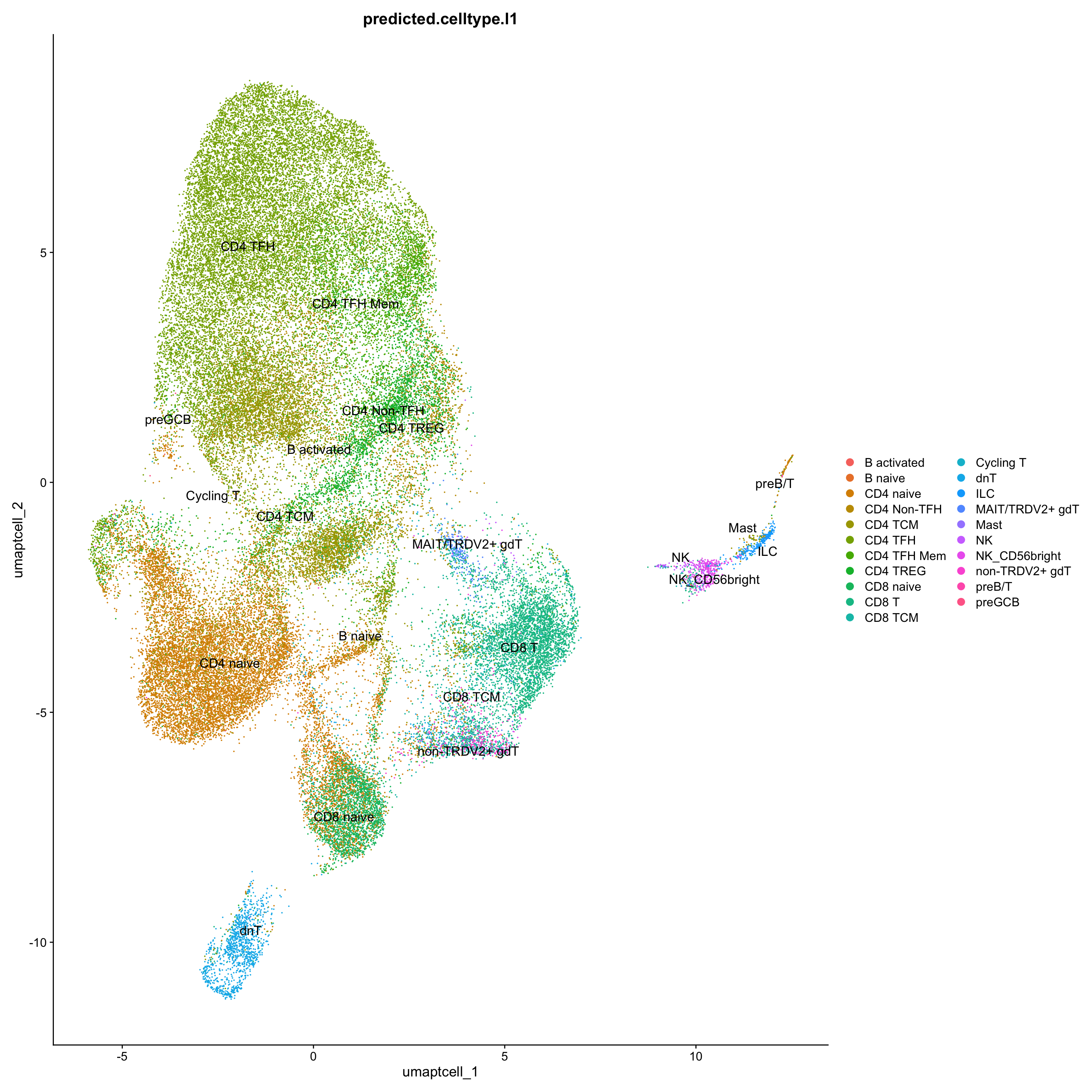
| Version | Author | Date |
|---|---|---|
| 54e4ec2 | Gunjan Dixit | 2025-01-08 |
sort(table(paed_sub$predicted.celltype.l1), decreasing = T)
        CD4 TFH       CD4 naive         CD4 TCM           CD8 T        CD4 TREG
          17830           11627            8592            4278            4076
    CD4 TFH Mem       CD8 naive     CD4 Non-TFH             dnT         CD8 TCM
           3609            2472            2050            1434            1429
 non-TRDV2+ gdT   NK_CD56bright             ILC MAIT/TRDV2+ gdT              NK
            408             324             305             228             135
      Cycling T     B activated          preGCB          preB/T         B naive
             24               4               3               2               1
           Mast
              1
# Plots for Level 1
DimPlot(paed_sub, reduction = "umap.tcell", group.by = "predicted.celltype.l1", raster = FALSE, repel = TRUE, label = TRUE, label.size = 5) +
paletteer::scale_colour_paletteer_d("Polychrome::palette36")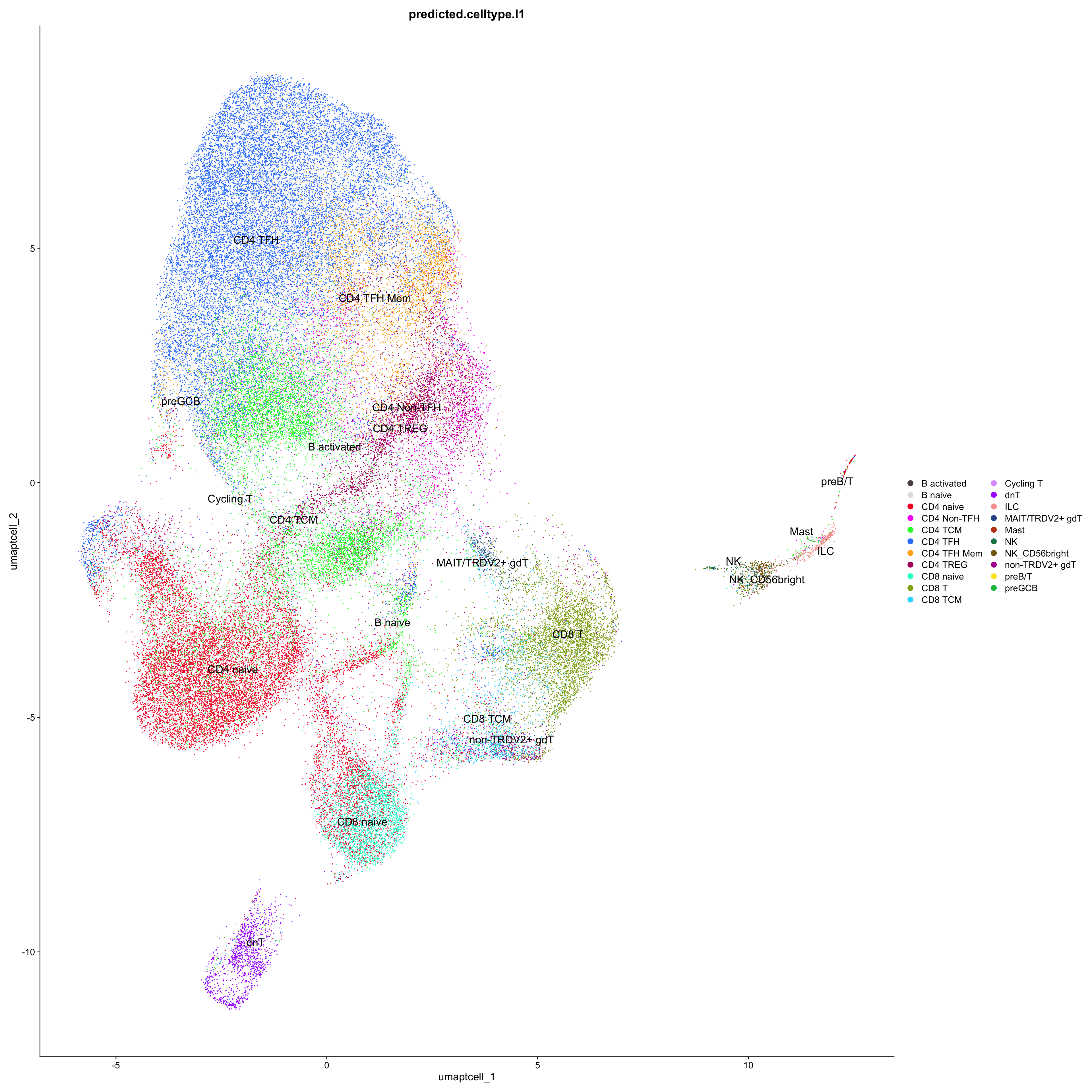
df_table_l1 <- as.data.frame(table(paed_sub$RNA_snn_res.0.4, paed_sub$predicted.celltype.l1))

ggplot(df_table_l1, aes(Var1, Freq, fill = Var2)) +
  geom_bar(stat = "identity") +
  labs(x = "RNA_snn_res.0.4", y = "Count", fill = "predicted.celltype.l1") +
  theme_minimal() +
  paletteer::scale_fill_paletteer_d("Polychrome::palette36") +
  ggtitle("Stacked Bar Plot of Tcell subsets (res=0.4) and predicted.celltype.l1")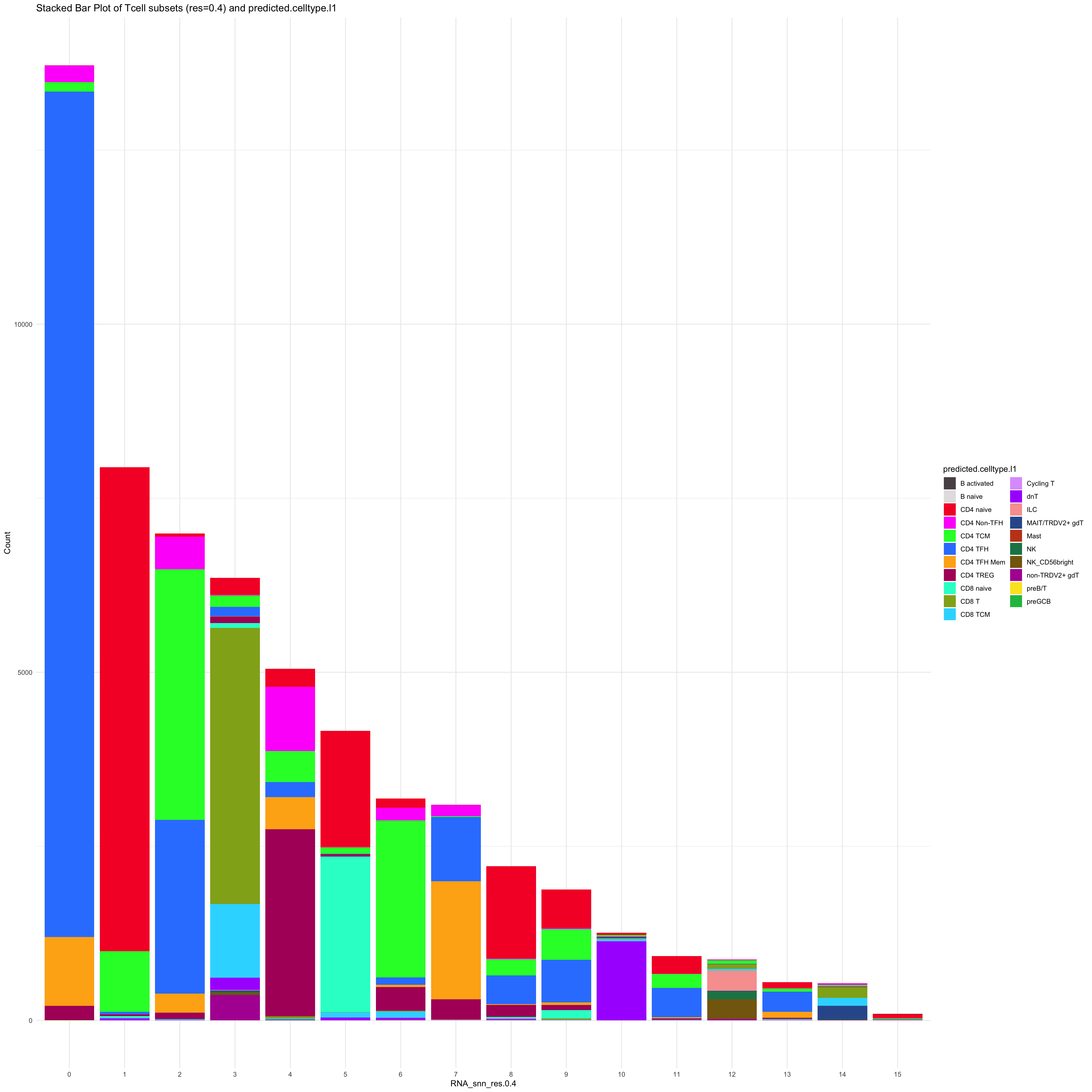
Old data- cells from previous clusters higlighted
Loading old Subclustering seurat object of T cell population and comparing with the updated clustering.
out2 <- here("output",
            "RDS", "AllBatches_Subclustering_SEUs", tissue,
             paste0("G000231_Neeland_",tissue,".Tcell_population.subclusters.SEU.rds"))

old_obj <- readRDS(out2)
cell_types <- unique(old_obj$cell_labels_v2)
for (cell_type in cell_types) {
cl_cells <- WhichCells(old_obj, idents = cell_type)
p <- DimPlot(
paed_sub,
reduction = "umap.tcell",
label = TRUE,
label.size = 4.5,
repel = TRUE,
raster = FALSE,
cells.highlight = cl_cells
) +
ggtitle(paste("Updated- Highlighted:", cell_type))
p1 <- DimPlot(
old_obj,
reduction = "umap.new",
label = T,
label.size = 4.5,
repel = TRUE,
raster = FALSE,
cells.highlight = cl_cells
) +
ggtitle(paste("Old Data- Highlighted:", cell_type))
print(p | p1)
}
| Version | Author | Date |
|---|---|---|
| 54e4ec2 | Gunjan Dixit | 2025-01-08 |
| Version | Author | Date |
|---|---|---|
| 54e4ec2 | Gunjan Dixit | 2025-01-08 |
| Version | Author | Date |
|---|---|---|
| 54e4ec2 | Gunjan Dixit | 2025-01-08 |
| Version | Author | Date |
|---|---|---|
| 54e4ec2 | Gunjan Dixit | 2025-01-08 |
| Version | Author | Date |
|---|---|---|
| 54e4ec2 | Gunjan Dixit | 2025-01-08 |
| Version | Author | Date |
|---|---|---|
| 54e4ec2 | Gunjan Dixit | 2025-01-08 |
| Version | Author | Date |
|---|---|---|
| 54e4ec2 | Gunjan Dixit | 2025-01-08 |
| Version | Author | Date |
|---|---|---|
| 54e4ec2 | Gunjan Dixit | 2025-01-08 |
| Version | Author | Date |
|---|---|---|
| 54e4ec2 | Gunjan Dixit | 2025-01-08 |
| Version | Author | Date |
|---|---|---|
| 54e4ec2 | Gunjan Dixit | 2025-01-08 |
| Version | Author | Date |
|---|---|---|
| 54e4ec2 | Gunjan Dixit | 2025-01-08 |
| Version | Author | Date |
|---|---|---|
| 54e4ec2 | Gunjan Dixit | 2025-01-08 |
| Version | Author | Date |
|---|---|---|
| 54e4ec2 | Gunjan Dixit | 2025-01-08 |
| Version | Author | Date |
|---|---|---|
| 54e4ec2 | Gunjan Dixit | 2025-01-08 |
Save subclustered SEU object (Tcells)
out2 <- here("output",
            "RDS", "AllBatches_Subclustering_SEUs_v2", tissue,
             paste0("G000231_Neeland_",tissue,".Tcell_population.subclusters.SEU.rds"))
#dir.create(out2)
#if (!file.exists(out2)) {
  saveRDS(paed_sub, file = out2)
#}
Updated cell-type labels (T cell clusters)
cell_labels <- readxl::read_excel(here("data/cell_labels_Mel_v4_Dec2024/earlyAIR_Tonsils_all.xlsx"), sheet = "T-reclustering")

new_cluster_names <- cell_labels %>%
  dplyr::select(cluster, annotation) %>%
  deframe()

paed_sub <- RenameIdents(paed_sub, new_cluster_names)
paed_sub@meta.data$cell_labels_v2 <- Idents(paed_sub)

p3 <- DimPlot(paed_sub, reduction = "umap.tcell", raster = FALSE, repel = TRUE, label = TRUE, label.size = 3.5) + ggtitle(paste0(tissue, ": UMAP with Updated T cell population"))

p3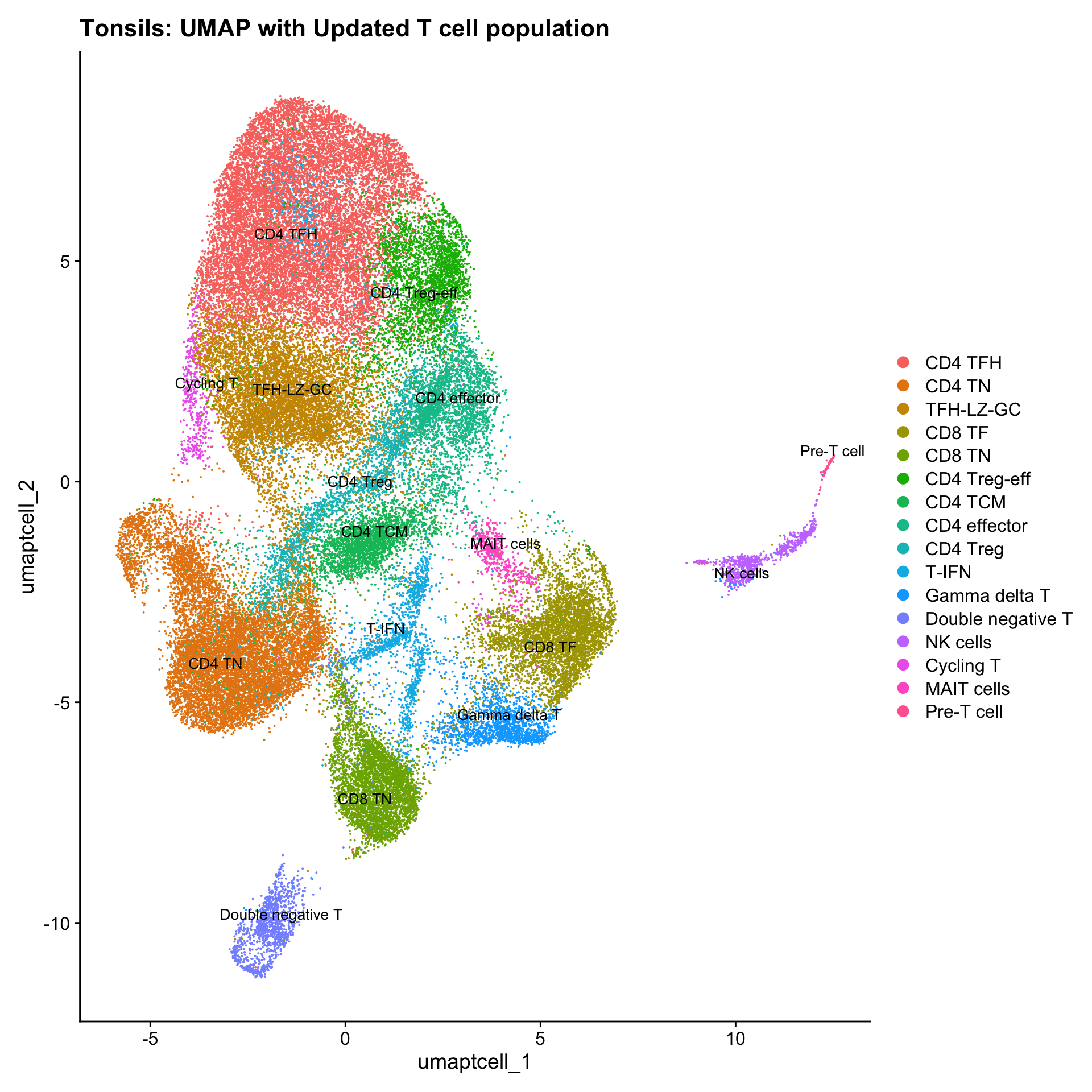
| Version | Author | Date |
|---|---|---|
| 54e4ec2 | Gunjan Dixit | 2025-01-08 |
Save subclustered SEU object
out2 <- here("output",
            "RDS", "AllBatches_Annotated_Subclustering_SEUs_v2", tissue,
             paste0("G000231_Neeland_",tissue,".Tcell_population.subclusters.SEU.rds"))
#dir.create(out2)
if (!file.exists(out2)) {
  saveRDS(paed_sub, file = out2)
}
Reclustering Germinal Center B cells
1, 6, 7, 10, 13, 14 Reclustering clusters
The marker genes for this reclustering can be found here-
#sub_clusters <- c(1, 6, 7, 10, 13, 14)

#idx <- which(merged_obj$cluster %in% sub_clusters)

idx <- which(Idents(merged_obj) %in% "Germinal centre B cells for reclustering")
paed_gc <- merged_obj[,idx]
paed_gc
An object of class Seurat
17566 features across 59526 samples within 1 assay
Active assay: RNA (17566 features, 2000 variable features)
3 layers present: data, counts, scale.data
4 dimensional reductions calculated: pca, umap.unintegrated, harmony, umap.harmony# Visualize the clustering results
DimPlot(paed_gc, reduction = "umap.harmony", group.by = "cluster", label = TRUE, label.size = 2.5, repel = TRUE, raster = FALSE )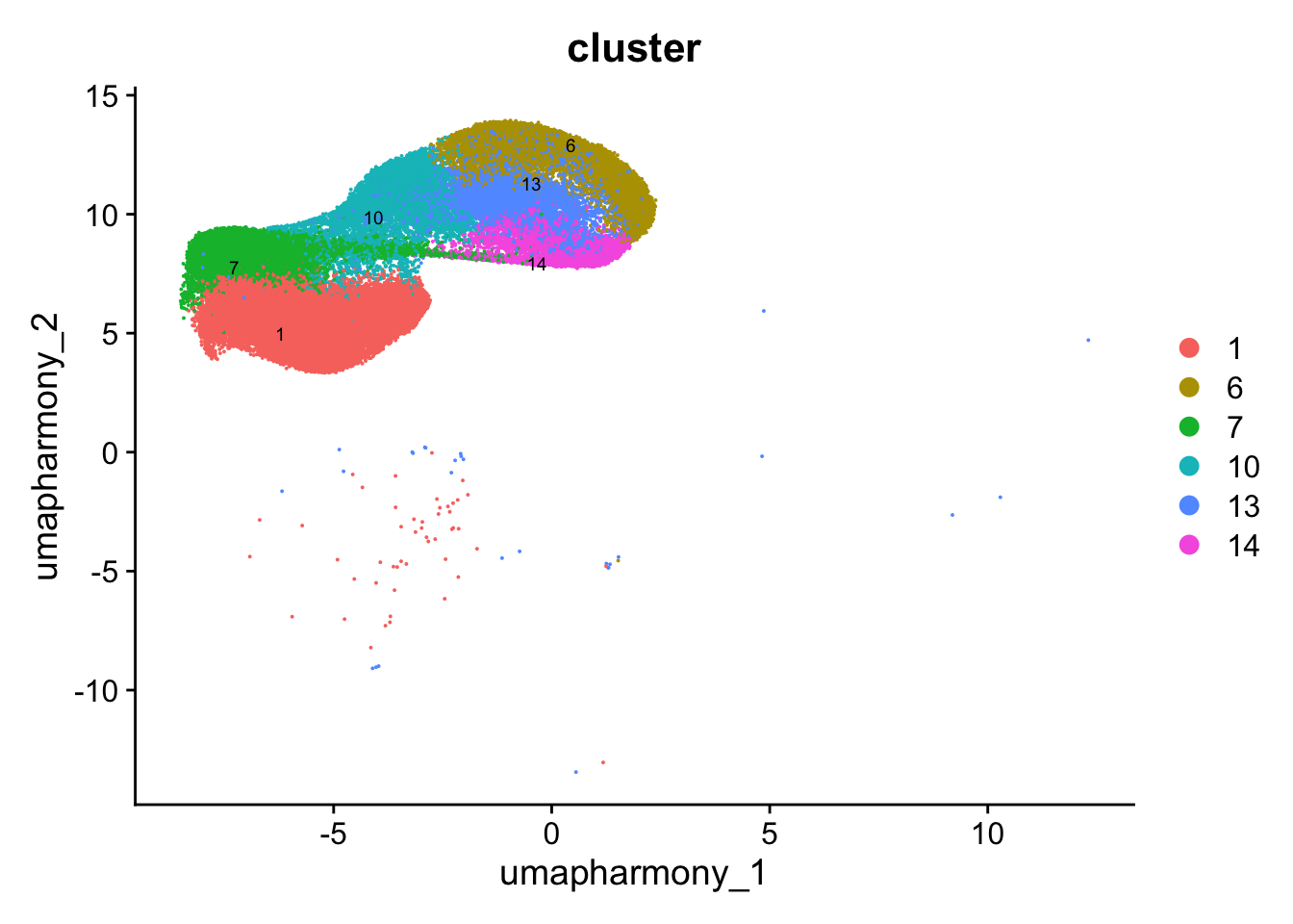
| Version | Author | Date |
|---|---|---|
| 54e4ec2 | Gunjan Dixit | 2025-01-08 |
paed_gc <- paed_gc %>%
  NormalizeData() %>%
  FindVariableFeatures() %>%
  ScaleData() %>%
  RunPCA()

paed_gc <- RunUMAP(paed_gc, dims = 1:30, reduction = "pca", reduction.name = "umap.gc")
meta_data_columns <- colnames(paed_gc@meta.data)
columns_to_remove <- grep("^RNA_snn_res", meta_data_columns, value = TRUE)
paed_gc@meta.data <- paed_gc@meta.data[, !(colnames(paed_gc@meta.data) %in% columns_to_remove)]resolutions <- seq(0.1, 1, by = 0.1)
paed_gc <- FindNeighbors(paed_gc, dims = 1:30, reduction = "pca")
paed_gc <- FindClusters(paed_gc, resolution = resolutions )Modularity Optimizer version 1.3.0 by Ludo Waltman and Nees Jan van Eck
Number of nodes: 59526
Number of edges: 1809714
Running Louvain algorithm...
Maximum modularity in 10 random starts: 0.9449
Number of communities: 3
Elapsed time: 11 seconds
Modularity Optimizer version 1.3.0 by Ludo Waltman and Nees Jan van Eck
Number of nodes: 59526
Number of edges: 1809714
Running Louvain algorithm...
Maximum modularity in 10 random starts: 0.9174
Number of communities: 6
Elapsed time: 10 seconds
Modularity Optimizer version 1.3.0 by Ludo Waltman and Nees Jan van Eck
Number of nodes: 59526
Number of edges: 1809714
Running Louvain algorithm...
Maximum modularity in 10 random starts: 0.9018
Number of communities: 8
Elapsed time: 9 seconds
Modularity Optimizer version 1.3.0 by Ludo Waltman and Nees Jan van Eck
Number of nodes: 59526
Number of edges: 1809714
Running Louvain algorithm...
Maximum modularity in 10 random starts: 0.8898
Number of communities: 12
Elapsed time: 10 seconds
Modularity Optimizer version 1.3.0 by Ludo Waltman and Nees Jan van Eck
Number of nodes: 59526
Number of edges: 1809714
Running Louvain algorithm...
Maximum modularity in 10 random starts: 0.8791
Number of communities: 14
Elapsed time: 10 seconds
Modularity Optimizer version 1.3.0 by Ludo Waltman and Nees Jan van Eck
Number of nodes: 59526
Number of edges: 1809714
Running Louvain algorithm...
Maximum modularity in 10 random starts: 0.8708
Number of communities: 13
Elapsed time: 9 seconds
Modularity Optimizer version 1.3.0 by Ludo Waltman and Nees Jan van Eck
Number of nodes: 59526
Number of edges: 1809714
Running Louvain algorithm...
Maximum modularity in 10 random starts: 0.8622
Number of communities: 15
Elapsed time: 10 seconds
Modularity Optimizer version 1.3.0 by Ludo Waltman and Nees Jan van Eck
Number of nodes: 59526
Number of edges: 1809714
Running Louvain algorithm...
Maximum modularity in 10 random starts: 0.8540
Number of communities: 17
Elapsed time: 10 seconds
Modularity Optimizer version 1.3.0 by Ludo Waltman and Nees Jan van Eck
Number of nodes: 59526
Number of edges: 1809714
Running Louvain algorithm...
Maximum modularity in 10 random starts: 0.8467
Number of communities: 19
Elapsed time: 9 seconds
Modularity Optimizer version 1.3.0 by Ludo Waltman and Nees Jan van Eck
Number of nodes: 59526
Number of edges: 1809714
Running Louvain algorithm...
Maximum modularity in 10 random starts: 0.8399
Number of communities: 19
Elapsed time: 10 secondsclustree(paed_gc, prefix = "RNA_snn_res.")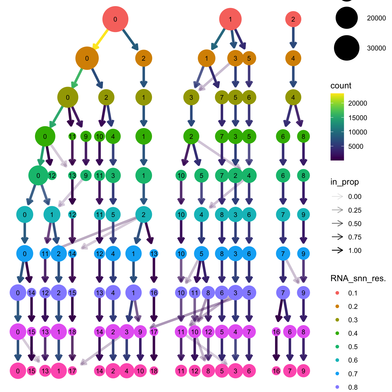
| Version | Author | Date |
|---|---|---|
| 54e4ec2 | Gunjan Dixit | 2025-01-08 |
# Visualize the clustering results
DimPlot(paed_gc, group.by = "RNA_snn_res.0.6", reduction = "umap.gc", label = TRUE, label.size = 2.5, repel = TRUE, raster = FALSE )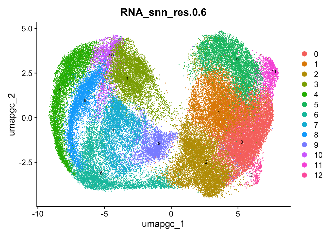
opt_res <- "RNA_snn_res.0.6"
n <- nlevels(paed_gc$RNA_snn_res.0.6)
paed_gc$RNA_snn_res.0.6 <- factor(paed_gc$RNA_snn_res.0.6, levels = seq(0,n-1))
paed_gc$seurat_clusters <- NULL
paed_gc$cluster <- paed_gc$RNA_snn_res.0.6
Idents(paed_gc) <- paed_gc$cluster
paed_gc.markers <- FindAllMarkers(paed_gc, only.pos = TRUE, min.pct = 0.25, logfc.threshold = 0.25)Calculating cluster 0Calculating cluster 1Calculating cluster 2Calculating cluster 3Calculating cluster 4Calculating cluster 5Calculating cluster 6Calculating cluster 7Calculating cluster 8Calculating cluster 9Calculating cluster 10Calculating cluster 11Calculating cluster 12paed_gc.markers %>%
group_by(cluster) %>% unique() %>%
top_n(n = 5, wt = avg_log2FC) -> top5
paed_gc.markers %>%
group_by(cluster) %>%
slice_head(n=1) %>%
pull(gene) -> best.wilcox.gene.per.cluster
best.wilcox.gene.per.cluster [1] "SEMA7A" "FCRL3" "AICDA" "MCM4" "HIST1H2AE" "BCL2A1"
[7] "CDC20" "TYMS" "HIST1H2BH" "TRBC2" "MTHFD1L" "PRDM1"
[13] "SLFN5" Feature plot shows the expression of top marker genes per cluster.
FeaturePlot(paed_gc,features=best.wilcox.gene.per.cluster, reduction = 'umap.gc', raster = FALSE, ncol = 2, label = TRUE)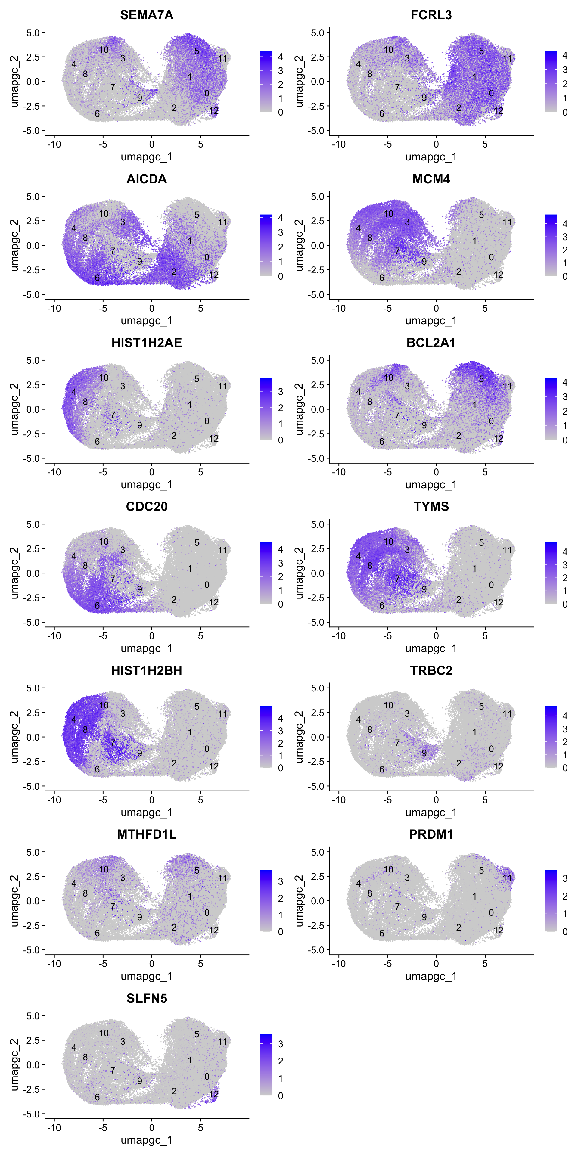
Top 10 marker genes from Seurat
## Seurat top markers
top10 <- paed_gc.markers %>%
    group_by(cluster) %>%
    top_n(n = 10, wt = avg_log2FC) %>%
    ungroup() %>%
    distinct(gene, .keep_all = TRUE) %>%
    arrange(cluster, desc(avg_log2FC))

cluster_colors <- paletteer::paletteer_d("pals::glasbey")[factor(top10$cluster)]

DotPlot(paed_gc,
        features = unique(top10$gene),
        group.by = opt_res,
        cols = c("azure1", "blueviolet"),
        dot.scale = 3, assay = "RNA") +
    RotatedAxis() +
    FontSize(y.text = 8, x.text = 12) +
    labs(y = element_blank(), x = element_blank()) +
    coord_flip() +
    theme(axis.text.y = element_text(color = cluster_colors)) +
    ggtitle("Top 10 marker genes per cluster (Seurat)")
Warning: Vectorized input to `element_text()` is not officially supported.
ℹ Results may be unexpected or may change in future versions of ggplot2.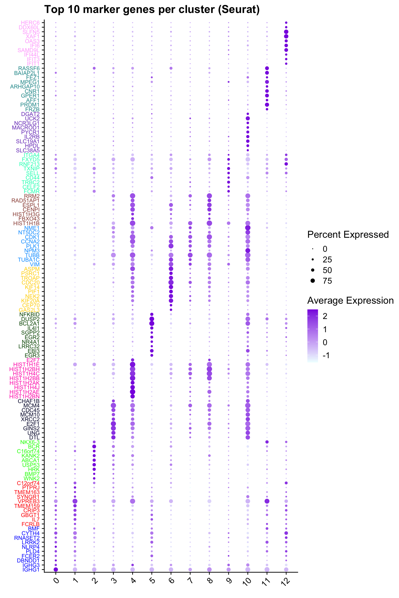
out_markers <- here("output",
            "CSV_v2",tissue,
            paste(tissue,"_Marker_genes_Reclustered_GC_population.",opt_res, sep = ""))

dir.create(out_markers, recursive = TRUE, showWarnings = FALSE)

for (cl in unique(paed_gc.markers$cluster)) {
  cluster_data <- paed_gc.markers %>% dplyr::filter(cluster == cl)
  file_name <- here(out_markers, paste0("G000231_Neeland_",tissue, "_cluster_", cl, ".csv"))
  if (!file.exists(file_name)) {
  write.csv(cluster_data, file = file_name)
  }
}
Corresponding Azimuth labels (GC cell subsets)
## Level 1
DimPlot(paed_gc, reduction = "umap.gc", group.by = "predicted.celltype.l1", raster = FALSE, repel = TRUE, label = TRUE, label.size = 4.5) 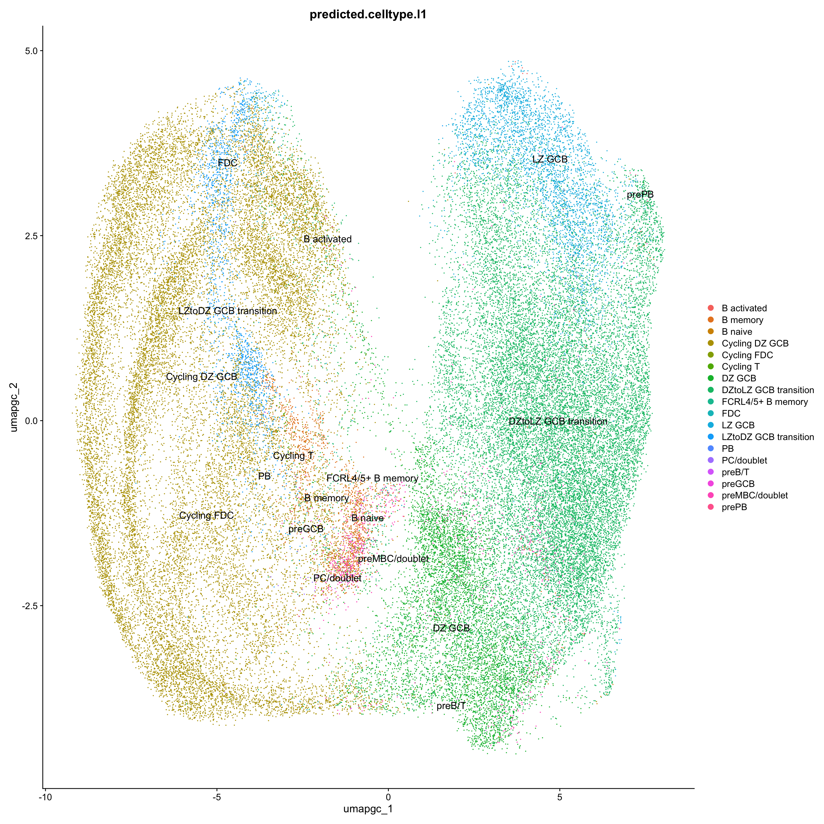
df_table <- as.data.frame(table(paed_gc$RNA_snn_res.0.6, paed_gc$predicted.celltype.l1))
ggplot(df_table, aes(Var1, Freq, fill = Var2)) +
  geom_bar(stat = "identity") +
  labs(x = "RNA_snn_res.0.6", y = "Count", fill = "predicted.celltype.l1") +
  theme_minimal() +
  ggtitle("Stacked Bar Plot of Tcell subsets (res=0.6) and predicted.celltype.l1")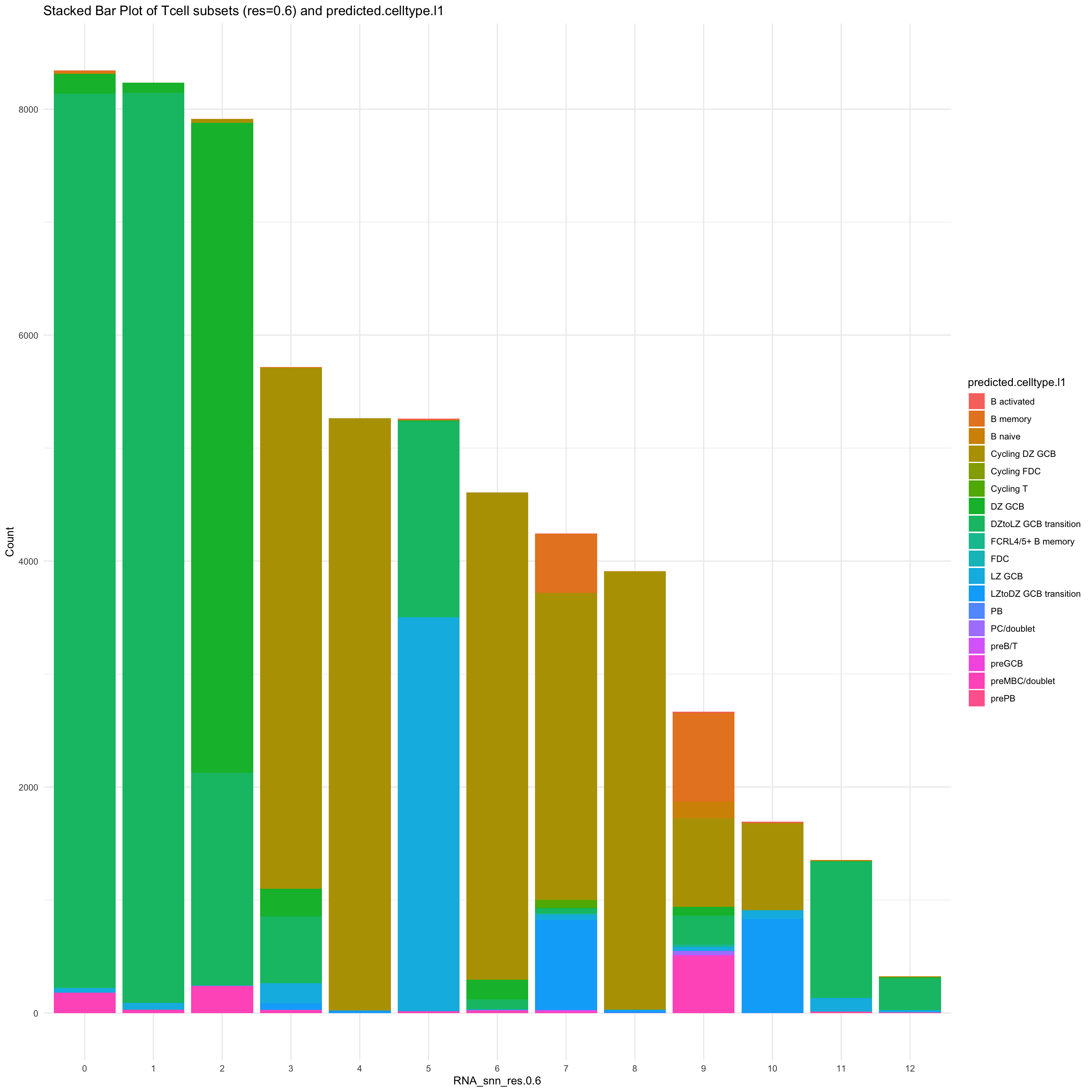
palette1 <- paletteer::paletteer_d("ggthemes::Classic_20")
palette2 <- paletteer::paletteer_d("Polychrome::light")
combined_palette <- unique(c(palette1, palette2))

labels <- "RNA_snn_res.0.6"

p <- vector("list",length(labels))
for(label in labels){
  paed_gc@meta.data %>%
    ggplot(aes(x = !!sym(label),
               fill = !!sym(label))) +
    geom_bar() +
    geom_text(aes(label = ..count..), stat = "count",
              vjust = -0.5, colour = "black", size = 2) +
    scale_y_log10() +
    theme(axis.text.x = element_blank(),
          axis.title.x = element_blank(),
          axis.ticks.x = element_blank()) +
    NoLegend() +
    labs(y = "No. Cells (log scale)") -> p1

  paed_gc@meta.data %>%
    dplyr::select(!!sym(label), donor_id) %>%
    group_by(!!sym(label), donor_id) %>%
    summarise(num = n()) %>%
    mutate(prop = num / sum(num)) %>%
  ggplot(aes(x = !!sym(label), y = prop * 100,
             fill = donor_id)) +
    geom_bar(stat = "identity") +
    theme(axis.text.x = element_text(angle = 90,
                                     vjust = 0.5,
                                     hjust = 1,
                                     size = 8)) +
    labs(y = "% Cells", fill = "Donor") +
  scale_fill_manual(values = combined_palette) -> p2

  (p1 / p2) & theme(legend.text = element_text(size = 8),
                  legend.key.size = unit(3, "mm")) -> p[[label]]
}
`summarise()` has grouped output by 'RNA_snn_res.0.6'. You can override using
the `.groups` argument.p[[1]]
NULL
$RNA_snn_res.0.6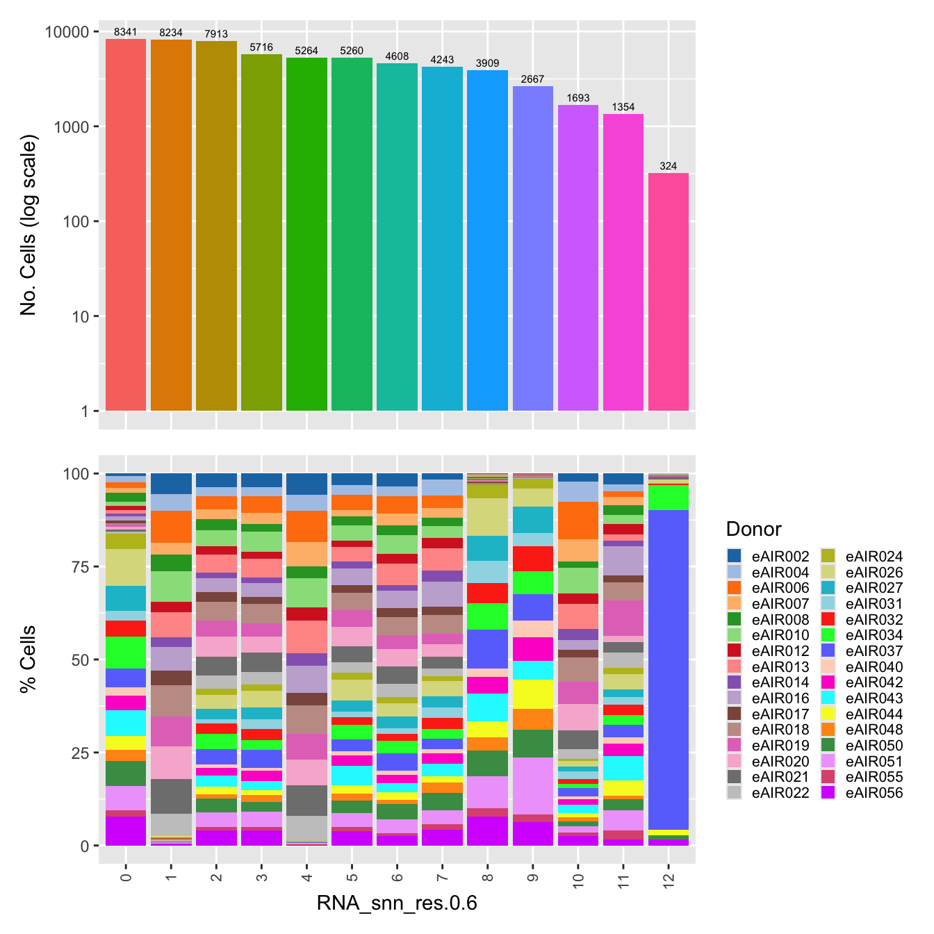
| Version | Author | Date |
|---|---|---|
| 54e4ec2 | Gunjan Dixit | 2025-01-08 |
Old data- cells from previous clusters higlighted
Loading old Subclustering seurat object of T cell population and comparing with the updated clustering.
out2 <- here("output",
            "RDS", "AllBatches_Subclustering_SEUs", tissue,
             paste0("G000231_Neeland_",tissue,".GC_population.subclusters.SEU.rds"))

old_obj <- readRDS(out2)
cell_types <- unique(old_obj$cell_labels_v2)
for (cell_type in cell_types) {
cl_cells <- WhichCells(old_obj, idents = cell_type)
p <- DimPlot(
paed_gc,
reduction = "umap.gc",
label = TRUE,
label.size = 4.5,
repel = TRUE,
raster = FALSE,
cells.highlight = cl_cells
) +
ggtitle(paste("Updated- Highlighted:", cell_type))
p1 <- DimPlot(
old_obj,
reduction = "umap.new",
label = T,
label.size = 4.5,
repel = TRUE,
raster = FALSE,
cells.highlight = cl_cells
) +
ggtitle(paste("Old Data- Highlighted:", cell_type))
print(p | p1)
}
| Version | Author | Date |
|---|---|---|
| 54e4ec2 | Gunjan Dixit | 2025-01-08 |
| Version | Author | Date |
|---|---|---|
| 54e4ec2 | Gunjan Dixit | 2025-01-08 |
| Version | Author | Date |
|---|---|---|
| 54e4ec2 | Gunjan Dixit | 2025-01-08 |
| Version | Author | Date |
|---|---|---|
| 54e4ec2 | Gunjan Dixit | 2025-01-08 |
| Version | Author | Date |
|---|---|---|
| 54e4ec2 | Gunjan Dixit | 2025-01-08 |
| Version | Author | Date |
|---|---|---|
| 54e4ec2 | Gunjan Dixit | 2025-01-08 |
| Version | Author | Date |
|---|---|---|
| 54e4ec2 | Gunjan Dixit | 2025-01-08 |
| Version | Author | Date |
|---|---|---|
| 54e4ec2 | Gunjan Dixit | 2025-01-08 |
| Version | Author | Date |
|---|---|---|
| 54e4ec2 | Gunjan Dixit | 2025-01-08 |
| Version | Author | Date |
|---|---|---|
| 54e4ec2 | Gunjan Dixit | 2025-01-08 |
| Version | Author | Date |
|---|---|---|
| 54e4ec2 | Gunjan Dixit | 2025-01-08 |
| Version | Author | Date |
|---|---|---|
| 54e4ec2 | Gunjan Dixit | 2025-01-08 |
Save subclustered SEU object
out2 <- here("output",
            "RDS", "AllBatches_Subclustering_SEUs_v2", tissue,
             paste0("G000231_Neeland_",tissue,".GC_population.subclusters.SEU.rds"))
#dir.create(out2)
#if (!file.exists(out2)) {
  saveRDS(paed_gc, file = out2)
#}
Updated cell-type labels (GC cell clusters)
cell_labels <- readxl::read_excel(here("data/cell_labels_Mel_v4_Dec2024/earlyAIR_Tonsils_all.xlsx"), sheet = "GC-B reclustering")

new_cluster_names <- cell_labels %>%
  dplyr::select(cluster, annotation) %>%
  deframe()

paed_gc <- RenameIdents(paed_gc, new_cluster_names)
paed_gc@meta.data$cell_labels_v2 <- Idents(paed_gc)

p3 <- DimPlot(paed_gc, reduction = "umap.gc", raster = FALSE, repel = TRUE, label = TRUE, label.size = 3.5) + ggtitle(paste0(tissue, ": UMAP with Updated GC cell population"))

p3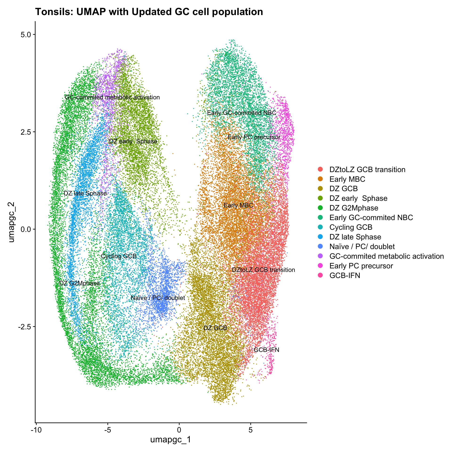
| Version | Author | Date |
|---|---|---|
| 54e4ec2 | Gunjan Dixit | 2025-01-08 |
Save subclustered SEU object Germinal Centre Bcells
out2 <- here("output",
            "RDS", "AllBatches_Annotated_Subclustering_SEUs_v2", tissue,
             paste0("G000231_Neeland_",tissue,".GC_population.subclusters.SEU.rds"))
#dir.create(out2)
if (!file.exists(out2)) {
  saveRDS(paed_gc, file = out2)
}
Other Clusters (excluding subclusters)
idx <- which(Idents(merged_obj) %in% c("T cells for reclustering", "Germinal centre B cells for reclustering"))
paed_other <- merged_obj[,-idx]
paed_other
An object of class Seurat
17566 features across 92386 samples within 1 assay
Active assay: RNA (17566 features, 2000 variable features)
3 layers present: data, counts, scale.data
4 dimensional reductions calculated: pca, umap.unintegrated, harmony, umap.harmonySave subclustered SEU object ( All other cells)
paed_other$cell_labels_v2 <-paed_other$cell_labels
out2 <- here("output",
            "RDS", "AllBatches_Annotated_Subclustering_SEUs_v2", tissue,
             paste0("G000231_Neeland_",tissue,".all_other.subclusters.SEU.rds"))

if (!file.exists(out2)) {
  saveRDS(paed_other, file = out2)
}
Merge seurat objects of subclusters
files <- list.files(here("output",
            "RDS", "AllBatches_Annotated_Subclustering_SEUs_v2", tissue),
                    full.names = TRUE)

seuLst <- lapply(files, function(f) readRDS(f))

seu <- merge(seuLst[[1]],
             y = c(seuLst[[2]],
                   seuLst[[3]]))
seu
An object of class Seurat
17566 features across 210744 samples within 1 assay
Active assay: RNA (17566 features, 2000 variable features)
9 layers present: data.1, data.2, data.3, counts.1, scale.data.1, counts.2, scale.data.2, counts.3, scale.data.3merged <- seu %>%
NormalizeData() %>%
FindVariableFeatures() %>%
ScaleData() %>%
RunPCA()Normalizing layer: counts.1Normalizing layer: counts.2Normalizing layer: counts.3Finding variable features for layer counts.1Finding variable features for layer counts.2Finding variable features for layer counts.3Centering and scaling data matrixPC_ 1
Positive: MKI67, KIFC1, NUSAP1, AURKB, TYMS, CDK1, NCAPG, STMN1, TK1, TOP2A
ZWINT, MYBL2, HMGB2, TPX2, BIRC5, KIF11, FOXM1, RRM2, ASF1B, HJURP
CCNA2, HIST1H1B, CCNB2, UHRF1, KIF2C, MND1, SPC25, CDCA8, SPC24, BUB1
Negative: CD44, TRBC2, SELL, FYB1, CD3D, CD3E, GIMAP7, TCF7, GIMAP4, IL32
CD2, LCP2, TC2N, KLF2, CD4, PLAC8, CD69, TRBC1, CD7, SRGN
CD96, CD28, BCL11B, IL7R, CCR7, ITM2A, DDIT4, ARL4C, GIMAP5, GPR183
PC_ 2
Positive: CD79A, IGHM, BCL11A, IGHD, CD83, IFI30, FCRL5, MPEG1, CR1, CTSH
CTSZ, CCR6, CD24, ADAM19, SEMA7A, PARP15, RUBCNL, ENTPD1, FCRL3, FAM30A
POU2AF1, NEIL1, PLD4, TNFRSF13B, IGKC, TRAF4, CBFA2T3, KYNU, CD1C, ZEB2
Negative: CD3D, CD3E, CD2, IL32, FYB1, TCF7, GIMAP4, GIMAP7, LCP2, MAF
CD28, CD4, SRGN, TC2N, ITM2A, TRBC1, CD7, IL2RB, ICOS, BCL11B
SPN, SH2D1A, TIGIT, SIRPG, TRBC2, PYHIN1, GIMAP5, TOX2, IL6R, PDCD1
PC_ 3
Positive: TRBC2, TCF7, CD3D, CD3E, TC2N, IKZF3, CD2, ITM2A, TRBC1, CD28
BCL11B, CD40LG, CXCR5, ST8SIA1, CD27, THEMIS, GIMAP7, TOX2, ICOS, PYHIN1
TRIB2, SIRPG, TIGIT, CD7, SH2D1A, IL32, GLCCI1, PDCD1, LEF1, GIMAP4
Negative: LYZ, CSF2RA, CST3, FCER1G, TMEM176B, CSF1R, TYROBP, SERPINA1, CD68, MS4A6A
ENPP2, ITGAX, RASSF4, TNFAIP2, SERPINF1, SLC8A1, HCK, LGALS2, CD14, FGL2
MAFB, SULF2, TMEM176A, PLA2G7, IGSF6, KCTD12, IL18, MMP14, MMP9, SLAMF8
PC_ 4
Positive: KIF20A, PLK1, CENPA, KIF14, CDC20, HMMR, NEK2, PSRC1, CENPE, DLGAP5
ASPM, KIF23, TROAP, AURKA, DEPDC1, CENPF, CDCA8, CCNB2, PIF1, GTSE1
HJURP, CDCA3, TOP2A, CKAP2L, SGO2, NUF2, BUB1, FAM83D, TPX2, UBE2C
Negative: LHFPL2, RGS13, SLC7A5, DUSP2, NME1, BCL6, EML6, HERPUD1, DHRS9, SLBP
TXNDC5, SRM, CCDC88A, GINS2, CD38, POU2AF1, PKM, JCHAIN, PDCD1, SIAH2
E2F1, UNG, BCAT1, SEC11C, CDC6, CAMK1, MCM6, BCL2L11, PRMT1, MCM4
PC_ 5
Positive: JCHAIN, MZB1, IGHG1, XBP1, DERL3, TXNDC5, CKAP4, PRDM1, FKBP11, RASSF6
SSR4, SEC11C, VDR, HSP90B1, TNFRSF17, CD38, SLAMF7, PRDX4, TXNDC11, IGHG3
TENT5C, TRIB1, EML6, ACOXL, MAN1A1, SDF2L1, CRELD2, MYDGF, HERPUD1, CD9
Negative: PARP15, PLAC8, SELL, CCR6, ACTG1, HSP90AB1, CD44, CD83, SEMA7A, CD69
MT-CO3, MCM5, MPEG1, MAT2A, APEX1, BCL11A, TNFRSF13B, CR1, FBL, MYC
FLNA, LY6E, MT-ND6, RUNX3, MT-ATP6, MT-ND3, ATIC, CHI3L2, IER5, DDX21 merged <- RunUMAP(merged, dims = 1:30, reduction = "pca", reduction.name = "umap.merged")15:58:57 UMAP embedding parameters a = 0.9922 b = 1.11215:58:57 Read 210744 rows and found 30 numeric columns15:58:57 Using Annoy for neighbor search, n_neighbors = 3015:58:57 Building Annoy index with metric = cosine, n_trees = 500% 10 20 30 40 50 60 70 80 90 100%[----|----|----|----|----|----|----|----|----|----|**************************************************|
15:59:09 Writing NN index file to temp file /var/folders/q8/kw1r78g12qn793xm7g0zvk94x2bh70/T//RtmpfzcVBu/file3035758e0b77
15:59:09 Searching Annoy index using 1 thread, search_k = 3000
15:59:54 Annoy recall = 100%
15:59:55 Commencing smooth kNN distance calibration using 1 thread with target n_neighbors = 30
15:59:57 Initializing from normalized Laplacian + noise (using RSpectra)
16:00:08 Commencing optimization for 200 epochs, with 9444688 positive edges
16:01:02 Optimization finishedp4 <- DimPlot(merged, reduction = "umap.merged", group.by = "cell_labels_v2",raster = FALSE, repel = TRUE, label = TRUE, label.size = 4.5) + ggtitle(paste0(tissue, ": UMAP with annotations")) + NoLegend()
p4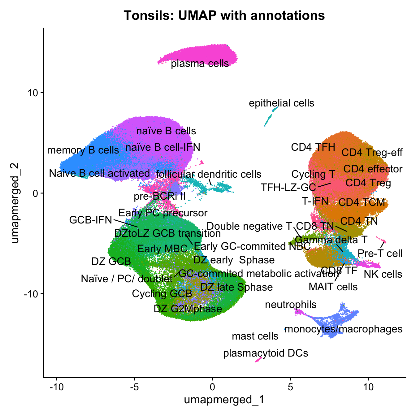
Save Final SEU object (All cells)
out3 <- here("output",
            "RDS", "AllBatches_Final_Clusters_SEUs_v2",
             paste0("G000231_Neeland_",tissue,".final_clusters.SEU.rds"))

#if (!file.exists(out3)) {
  saveRDS(merged, file = out3)
#}
labels <- c("cell_labels", "cell_labels_v2")
p <- vector("list",length(labels))
for(label in labels){
merged@meta.data %>%
ggplot(aes(x = !!sym(label),
fill = !!sym(label))) +
geom_bar() +
geom_text(aes(label = ..count..), stat = "count",
vjust = -0.5, colour = "black", size = 2) +
scale_y_log10() +
theme(axis.text.x = element_blank(),
axis.title.x = element_blank(),
axis.ticks.x = element_blank()) +
NoLegend() +
labs(y = "No. Cells (log scale)") -> p1
merged@meta.data %>%
dplyr::select(!!sym(label), donor_id) %>%
group_by(!!sym(label), donor_id) %>%
summarise(num = n()) %>%
mutate(prop = num / sum(num)) %>%
ggplot(aes(x = !!sym(label), y = prop * 100,
fill = donor_id)) +
geom_bar(stat = "identity") +
theme(axis.text.x = element_text(angle = 90,
vjust = 0.5,
hjust = 1,
size = 8)) +
labs(y = "% Cells", fill = "Donor") +
scale_fill_manual(values = combined_palette) -> p2
(p1 / p2) & theme(legend.text = element_text(size = 8),
legend.key.size = unit(3, "mm")) -> p[[label]]
}`summarise()` has grouped output by 'cell_labels'. You can override using the
`.groups` argument.
`summarise()` has grouped output by 'cell_labels_v2'. You can override using
the `.groups` argument.p[[1]]
NULL
[[2]]
NULL
$cell_labels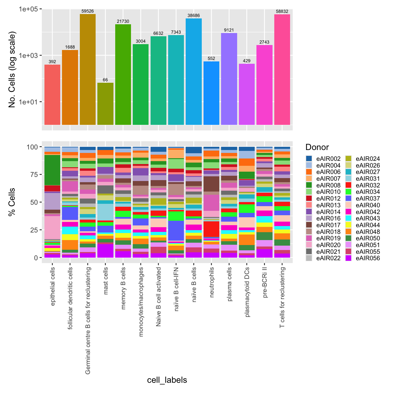
$cell_labels_v2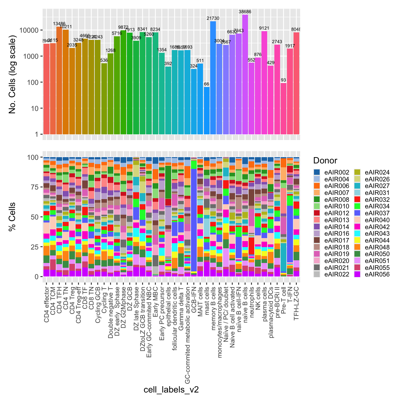
Session Info
sessioninfo::session_info()─ Session info ───────────────────────────────────────────────────────────────
setting value
version R version 4.3.2 (2023-10-31)
os macOS 15.2
system aarch64, darwin20
ui X11
language (EN)
collate en_US.UTF-8
ctype en_US.UTF-8
tz Australia/Melbourne
date 2025-01-16
pandoc 3.1.1 @ /Users/dixitgunjan/Desktop/RStudio.app/Contents/Resources/app/quarto/bin/tools/ (via rmarkdown)
─ Packages ───────────────────────────────────────────────────────────────────
package * version date (UTC) lib source
abind 1.4-5 2016-07-21 [1] CRAN (R 4.3.0)
backports 1.4.1 2021-12-13 [1] CRAN (R 4.3.0)
beeswarm 0.4.0 2021-06-01 [1] CRAN (R 4.3.0)
BiocManager 1.30.22 2023-08-08 [1] CRAN (R 4.3.0)
BiocStyle * 2.30.0 2023-10-26 [1] Bioconductor
bslib 0.6.1 2023-11-28 [1] CRAN (R 4.3.1)
cachem 1.0.8 2023-05-01 [1] CRAN (R 4.3.0)
callr 3.7.5 2024-02-19 [1] CRAN (R 4.3.1)
cellranger 1.1.0 2016-07-27 [1] CRAN (R 4.3.0)
checkmate 2.3.1 2023-12-04 [1] CRAN (R 4.3.1)
cli 3.6.2 2023-12-11 [1] CRAN (R 4.3.1)
cluster 2.1.6 2023-12-01 [1] CRAN (R 4.3.1)
clustree * 0.5.1 2023-11-05 [1] CRAN (R 4.3.1)
codetools 0.2-19 2023-02-01 [1] CRAN (R 4.3.2)
colorspace 2.1-0 2023-01-23 [1] CRAN (R 4.3.0)
cowplot 1.1.3 2024-01-22 [1] CRAN (R 4.3.1)
data.table * 1.15.0 2024-01-30 [1] CRAN (R 4.3.1)
deldir 2.0-2 2023-11-23 [1] CRAN (R 4.3.1)
digest 0.6.34 2024-01-11 [1] CRAN (R 4.3.1)
dotCall64 1.1-1 2023-11-28 [1] CRAN (R 4.3.1)
dplyr * 1.1.4 2023-11-17 [1] CRAN (R 4.3.1)
ellipsis 0.3.2 2021-04-29 [1] CRAN (R 4.3.0)
evaluate 0.23 2023-11-01 [1] CRAN (R 4.3.1)
fansi 1.0.6 2023-12-08 [1] CRAN (R 4.3.1)
farver 2.1.1 2022-07-06 [1] CRAN (R 4.3.0)
fastDummies 1.7.3 2023-07-06 [1] CRAN (R 4.3.0)
fastmap 1.1.1 2023-02-24 [1] CRAN (R 4.3.0)
fitdistrplus 1.1-11 2023-04-25 [1] CRAN (R 4.3.0)
forcats * 1.0.0 2023-01-29 [1] CRAN (R 4.3.0)
fs 1.6.3 2023-07-20 [1] CRAN (R 4.3.0)
future 1.33.1 2023-12-22 [1] CRAN (R 4.3.1)
future.apply 1.11.1 2023-12-21 [1] CRAN (R 4.3.1)
generics 0.1.3 2022-07-05 [1] CRAN (R 4.3.0)
getPass 0.2-4 2023-12-10 [1] CRAN (R 4.3.1)
ggbeeswarm 0.7.2 2023-04-29 [1] CRAN (R 4.3.0)
ggforce 0.4.2 2024-02-19 [1] CRAN (R 4.3.1)
ggplot2 * 3.5.0 2024-02-23 [1] CRAN (R 4.3.1)
ggraph * 2.1.0 2022-10-09 [1] CRAN (R 4.3.0)
ggrastr 1.0.2 2023-06-01 [1] CRAN (R 4.3.0)
ggrepel 0.9.5 2024-01-10 [1] CRAN (R 4.3.1)
ggridges 0.5.6 2024-01-23 [1] CRAN (R 4.3.1)
git2r 0.33.0 2023-11-26 [1] CRAN (R 4.3.1)
globals 0.16.2 2022-11-21 [1] CRAN (R 4.3.0)
glue 1.7.0 2024-01-09 [1] CRAN (R 4.3.1)
goftest 1.2-3 2021-10-07 [1] CRAN (R 4.3.0)
graphlayouts 1.1.0 2024-01-19 [1] CRAN (R 4.3.1)
gridExtra 2.3 2017-09-09 [1] CRAN (R 4.3.0)
gtable 0.3.4 2023-08-21 [1] CRAN (R 4.3.0)
here * 1.0.1 2020-12-13 [1] CRAN (R 4.3.0)
highr 0.10 2022-12-22 [1] CRAN (R 4.3.0)
hms 1.1.3 2023-03-21 [1] CRAN (R 4.3.0)
htmltools 0.5.7 2023-11-03 [1] CRAN (R 4.3.1)
htmlwidgets 1.6.4 2023-12-06 [1] CRAN (R 4.3.1)
httpuv 1.6.14 2024-01-26 [1] CRAN (R 4.3.1)
httr 1.4.7 2023-08-15 [1] CRAN (R 4.3.0)
ica 1.0-3 2022-07-08 [1] CRAN (R 4.3.0)
igraph 2.0.2 2024-02-17 [1] CRAN (R 4.3.1)
irlba 2.3.5.1 2022-10-03 [1] CRAN (R 4.3.2)
jquerylib 0.1.4 2021-04-26 [1] CRAN (R 4.3.0)
jsonlite 1.8.8 2023-12-04 [1] CRAN (R 4.3.1)
kableExtra * 1.4.0 2024-01-24 [1] CRAN (R 4.3.1)
KernSmooth 2.23-22 2023-07-10 [1] CRAN (R 4.3.2)
knitr 1.45 2023-10-30 [1] CRAN (R 4.3.1)
labeling 0.4.3 2023-08-29 [1] CRAN (R 4.3.0)
later 1.3.2 2023-12-06 [1] CRAN (R 4.3.1)
lattice 0.22-5 2023-10-24 [1] CRAN (R 4.3.1)
lazyeval 0.2.2 2019-03-15 [1] CRAN (R 4.3.0)
leiden 0.4.3.1 2023-11-17 [1] CRAN (R 4.3.1)
lifecycle 1.0.4 2023-11-07 [1] CRAN (R 4.3.1)
limma 3.58.1 2023-11-02 [1] Bioconductor
listenv 0.9.1 2024-01-29 [1] CRAN (R 4.3.1)
lmtest 0.9-40 2022-03-21 [1] CRAN (R 4.3.0)
lubridate * 1.9.3 2023-09-27 [1] CRAN (R 4.3.1)
magrittr 2.0.3 2022-03-30 [1] CRAN (R 4.3.0)
MASS 7.3-60.0.1 2024-01-13 [1] CRAN (R 4.3.1)
Matrix 1.6-5 2024-01-11 [1] CRAN (R 4.3.1)
matrixStats 1.2.0 2023-12-11 [1] CRAN (R 4.3.1)
mime 0.12 2021-09-28 [1] CRAN (R 4.3.0)
miniUI 0.1.1.1 2018-05-18 [1] CRAN (R 4.3.0)
munsell 0.5.0 2018-06-12 [1] CRAN (R 4.3.0)
nlme 3.1-164 2023-11-27 [1] CRAN (R 4.3.1)
paletteer 1.6.0 2024-01-21 [1] CRAN (R 4.3.1)
parallelly 1.37.0 2024-02-14 [1] CRAN (R 4.3.1)
patchwork * 1.2.0 2024-01-08 [1] CRAN (R 4.3.1)
pbapply 1.7-2 2023-06-27 [1] CRAN (R 4.3.0)
pillar 1.9.0 2023-03-22 [1] CRAN (R 4.3.0)
pkgconfig 2.0.3 2019-09-22 [1] CRAN (R 4.3.0)
plotly 4.10.4 2024-01-13 [1] CRAN (R 4.3.1)
plyr 1.8.9 2023-10-02 [1] CRAN (R 4.3.1)
png 0.1-8 2022-11-29 [1] CRAN (R 4.3.0)
polyclip 1.10-6 2023-09-27 [1] CRAN (R 4.3.1)
presto 1.0.0 2024-02-27 [1] Github (immunogenomics/presto@31dc97f)
prismatic 1.1.1 2022-08-15 [1] CRAN (R 4.3.0)
processx 3.8.3 2023-12-10 [1] CRAN (R 4.3.1)
progressr 0.14.0 2023-08-10 [1] CRAN (R 4.3.0)
promises 1.2.1 2023-08-10 [1] CRAN (R 4.3.0)
ps 1.7.6 2024-01-18 [1] CRAN (R 4.3.1)
purrr * 1.0.2 2023-08-10 [1] CRAN (R 4.3.0)
R6 2.5.1 2021-08-19 [1] CRAN (R 4.3.0)
RANN 2.6.1 2019-01-08 [1] CRAN (R 4.3.0)
RColorBrewer * 1.1-3 2022-04-03 [1] CRAN (R 4.3.0)
Rcpp 1.0.12 2024-01-09 [1] CRAN (R 4.3.1)
RcppAnnoy 0.0.22 2024-01-23 [1] CRAN (R 4.3.1)
RcppHNSW 0.6.0 2024-02-04 [1] CRAN (R 4.3.1)
readr * 2.1.5 2024-01-10 [1] CRAN (R 4.3.1)
readxl 1.4.3 2023-07-06 [1] CRAN (R 4.3.0)
rematch2 2.1.2 2020-05-01 [1] CRAN (R 4.3.0)
reshape2 1.4.4 2020-04-09 [1] CRAN (R 4.3.0)
reticulate 1.35.0 2024-01-31 [1] CRAN (R 4.3.1)
rlang 1.1.3 2024-01-10 [1] CRAN (R 4.3.1)
rmarkdown 2.25 2023-09-18 [1] CRAN (R 4.3.1)
ROCR 1.0-11 2020-05-02 [1] CRAN (R 4.3.0)
rprojroot 2.0.4 2023-11-05 [1] CRAN (R 4.3.1)
RSpectra 0.16-1 2022-04-24 [1] CRAN (R 4.3.0)
rstudioapi 0.15.0 2023-07-07 [1] CRAN (R 4.3.0)
Rtsne 0.17 2023-12-07 [1] CRAN (R 4.3.1)
sass 0.4.8 2023-12-06 [1] CRAN (R 4.3.1)
scales 1.3.0 2023-11-28 [1] CRAN (R 4.3.1)
scattermore 1.2 2023-06-12 [1] CRAN (R 4.3.0)
sctransform 0.4.1 2023-10-19 [1] CRAN (R 4.3.1)
sessioninfo 1.2.2 2021-12-06 [1] CRAN (R 4.3.0)
Seurat * 5.0.1.9009 2024-02-28 [1] Github (satijalab/seurat@6a3ef5e)
SeuratObject * 5.0.1 2023-11-17 [1] CRAN (R 4.3.1)
shiny 1.8.0 2023-11-17 [1] CRAN (R 4.3.1)
sp * 2.1-3 2024-01-30 [1] CRAN (R 4.3.1)
spam 2.10-0 2023-10-23 [1] CRAN (R 4.3.1)
spatstat.data 3.0-4 2024-01-15 [1] CRAN (R 4.3.1)
spatstat.explore 3.2-6 2024-02-01 [1] CRAN (R 4.3.1)
spatstat.geom 3.2-8 2024-01-26 [1] CRAN (R 4.3.1)
spatstat.random 3.2-2 2023-11-29 [1] CRAN (R 4.3.1)
spatstat.sparse 3.0-3 2023-10-24 [1] CRAN (R 4.3.1)
spatstat.utils 3.0-4 2023-10-24 [1] CRAN (R 4.3.1)
statmod 1.5.0 2023-01-06 [1] CRAN (R 4.3.0)
stringi 1.8.3 2023-12-11 [1] CRAN (R 4.3.1)
stringr * 1.5.1 2023-11-14 [1] CRAN (R 4.3.1)
survival 3.5-8 2024-02-14 [1] CRAN (R 4.3.1)
svglite 2.1.3 2023-12-08 [1] CRAN (R 4.3.1)
systemfonts 1.0.5 2023-10-09 [1] CRAN (R 4.3.1)
tensor 1.5 2012-05-05 [1] CRAN (R 4.3.0)
tibble * 3.2.1 2023-03-20 [1] CRAN (R 4.3.0)
tidygraph 1.3.1 2024-01-30 [1] CRAN (R 4.3.1)
tidyr * 1.3.1 2024-01-24 [1] CRAN (R 4.3.1)
tidyselect 1.2.0 2022-10-10 [1] CRAN (R 4.3.0)
tidyverse * 2.0.0 2023-02-22 [1] CRAN (R 4.3.0)
timechange 0.3.0 2024-01-18 [1] CRAN (R 4.3.1)
tweenr 2.0.3 2024-02-26 [1] CRAN (R 4.3.1)
tzdb 0.4.0 2023-05-12 [1] CRAN (R 4.3.0)
utf8 1.2.4 2023-10-22 [1] CRAN (R 4.3.1)
uwot 0.1.16 2023-06-29 [1] CRAN (R 4.3.0)
vctrs 0.6.5 2023-12-01 [1] CRAN (R 4.3.1)
vipor 0.4.7 2023-12-18 [1] CRAN (R 4.3.1)
viridis 0.6.5 2024-01-29 [1] CRAN (R 4.3.1)
viridisLite 0.4.2 2023-05-02 [1] CRAN (R 4.3.0)
whisker 0.4.1 2022-12-05 [1] CRAN (R 4.3.0)
withr 3.0.0 2024-01-16 [1] CRAN (R 4.3.1)
workflowr * 1.7.1 2023-08-23 [1] CRAN (R 4.3.0)
xfun 0.42 2024-02-08 [1] CRAN (R 4.3.1)
xml2 1.3.6 2023-12-04 [1] CRAN (R 4.3.1)
xtable 1.8-4 2019-04-21 [1] CRAN (R 4.3.0)
yaml 2.3.8 2023-12-11 [1] CRAN (R 4.3.1)
zoo 1.8-12 2023-04-13 [1] CRAN (R 4.3.0)
[1] /Library/Frameworks/R.framework/Versions/4.3-arm64/Resources/library
──────────────────────────────────────────────────────────────────────────────
sessionInfo()R version 4.3.2 (2023-10-31)
Platform: aarch64-apple-darwin20 (64-bit)
Running under: macOS 15.2
Matrix products: default
BLAS: /Library/Frameworks/R.framework/Versions/4.3-arm64/Resources/lib/libRblas.0.dylib
LAPACK: /Library/Frameworks/R.framework/Versions/4.3-arm64/Resources/lib/libRlapack.dylib; LAPACK version 3.11.0
locale:
[1] en_US.UTF-8/en_US.UTF-8/en_US.UTF-8/C/en_US.UTF-8/en_US.UTF-8
time zone: Australia/Melbourne
tzcode source: internal
attached base packages:
[1] stats graphics grDevices utils datasets methods base
other attached packages:
[1] patchwork_1.2.0 data.table_1.15.0 RColorBrewer_1.1-3 kableExtra_1.4.0
[5] clustree_0.5.1 ggraph_2.1.0 Seurat_5.0.1.9009 SeuratObject_5.0.1
[9] sp_2.1-3 here_1.0.1 lubridate_1.9.3 forcats_1.0.0
[13] stringr_1.5.1 dplyr_1.1.4 purrr_1.0.2 readr_2.1.5
[17] tidyr_1.3.1 tibble_3.2.1 ggplot2_3.5.0 tidyverse_2.0.0
[21] BiocStyle_2.30.0 workflowr_1.7.1
loaded via a namespace (and not attached):
[1] RcppAnnoy_0.0.22 splines_4.3.2 later_1.3.2
[4] prismatic_1.1.1 cellranger_1.1.0 polyclip_1.10-6
[7] fastDummies_1.7.3 lifecycle_1.0.4 rprojroot_2.0.4
[10] globals_0.16.2 processx_3.8.3 lattice_0.22-5
[13] MASS_7.3-60.0.1 backports_1.4.1 magrittr_2.0.3
[16] limma_3.58.1 plotly_4.10.4 sass_0.4.8
[19] rmarkdown_2.25 jquerylib_0.1.4 yaml_2.3.8
[22] httpuv_1.6.14 sctransform_0.4.1 spam_2.10-0
[25] sessioninfo_1.2.2 spatstat.sparse_3.0-3 reticulate_1.35.0
[28] cowplot_1.1.3 pbapply_1.7-2 abind_1.4-5
[31] Rtsne_0.17 presto_1.0.0 tweenr_2.0.3
[34] git2r_0.33.0 ggrepel_0.9.5 irlba_2.3.5.1
[37] listenv_0.9.1 spatstat.utils_3.0-4 goftest_1.2-3
[40] RSpectra_0.16-1 spatstat.random_3.2-2 fitdistrplus_1.1-11
[43] parallelly_1.37.0 svglite_2.1.3 leiden_0.4.3.1
[46] codetools_0.2-19 xml2_1.3.6 ggforce_0.4.2
[49] tidyselect_1.2.0 farver_2.1.1 viridis_0.6.5
[52] matrixStats_1.2.0 spatstat.explore_3.2-6 jsonlite_1.8.8
[55] ellipsis_0.3.2 tidygraph_1.3.1 progressr_0.14.0
[58] ggridges_0.5.6 survival_3.5-8 systemfonts_1.0.5
[61] tools_4.3.2 ica_1.0-3 Rcpp_1.0.12
[64] glue_1.7.0 gridExtra_2.3 xfun_0.42
[67] withr_3.0.0 BiocManager_1.30.22 fastmap_1.1.1
[70] fansi_1.0.6 callr_3.7.5 digest_0.6.34
[73] timechange_0.3.0 R6_2.5.1 mime_0.12
[76] colorspace_2.1-0 scattermore_1.2 tensor_1.5
[79] spatstat.data_3.0-4 utf8_1.2.4 generics_0.1.3
[82] graphlayouts_1.1.0 httr_1.4.7 htmlwidgets_1.6.4
[85] whisker_0.4.1 uwot_0.1.16 pkgconfig_2.0.3
[88] gtable_0.3.4 lmtest_0.9-40 htmltools_0.5.7
[91] dotCall64_1.1-1 scales_1.3.0 png_0.1-8
[94] knitr_1.45 rstudioapi_0.15.0 tzdb_0.4.0
[97] reshape2_1.4.4 checkmate_2.3.1 nlme_3.1-164
[100] cachem_1.0.8 zoo_1.8-12 KernSmooth_2.23-22
[103] vipor_0.4.7 parallel_4.3.2 miniUI_0.1.1.1
[106] ggrastr_1.0.2 pillar_1.9.0 grid_4.3.2
[109] vctrs_0.6.5 RANN_2.6.1 promises_1.2.1
[112] xtable_1.8-4 cluster_2.1.6 paletteer_1.6.0
[115] beeswarm_0.4.0 evaluate_0.23 cli_3.6.2
[118] compiler_4.3.2 rlang_1.1.3 future.apply_1.11.1
[121] labeling_0.4.3 rematch2_2.1.2 ps_1.7.6
[124] getPass_0.2-4 plyr_1.8.9 fs_1.6.3
[127] ggbeeswarm_0.7.2 stringi_1.8.3 viridisLite_0.4.2
[130] deldir_2.0-2 munsell_0.5.0 lazyeval_0.2.2
[133] spatstat.geom_3.2-8 Matrix_1.6-5 RcppHNSW_0.6.0
[136] hms_1.1.3 future_1.33.1 statmod_1.5.0
[139] shiny_1.8.0 highr_0.10 ROCR_1.0-11
[142] igraph_2.0.2 bslib_0.6.1 readxl_1.4.3