 Pishas
et al 2024
Pishas
et al 2024
Ovarian Cancer Screen
Epigenetics/Kinase/FDA
Compounds
Last updated: 2024-07-19
Checks: 6 1
Knit directory:
Pishas_et_al_2024_Ovarian_Compound_Screen/
This reproducible R Markdown analysis was created with workflowr (version 1.7.1). The Checks tab describes the reproducibility checks that were applied when the results were created. The Past versions tab lists the development history.
The R Markdown file has unstaged changes. To know which version of
the R Markdown file created these results, you’ll want to first commit
it to the Git repo. If you’re still working on the analysis, you can
ignore this warning. When you’re finished, you can run
wflow_publish to commit the R Markdown file and build the
HTML.
Great job! The global environment was empty. Objects defined in the global environment can affect the analysis in your R Markdown file in unknown ways. For reproduciblity it’s best to always run the code in an empty environment.
The command set.seed(20231219) was run prior to running
the code in the R Markdown file. Setting a seed ensures that any results
that rely on randomness, e.g. subsampling or permutations, are
reproducible.
Great job! Recording the operating system, R version, and package versions is critical for reproducibility.
Nice! There were no cached chunks for this analysis, so you can be confident that you successfully produced the results during this run.
Great job! Using relative paths to the files within your workflowr project makes it easier to run your code on other machines.
Great! You are using Git for version control. Tracking code development and connecting the code version to the results is critical for reproducibility.
The results in this page were generated with repository version f638c44. See the Past versions tab to see a history of the changes made to the R Markdown and HTML files.
Note that you need to be careful to ensure that all relevant files for
the analysis have been committed to Git prior to generating the results
(you can use wflow_publish or
wflow_git_commit). workflowr only checks the R Markdown
file, but you know if there are other scripts or data files that it
depends on. Below is the status of the Git repository when the results
were generated:
Ignored files:
    Ignored:    .Rhistory
    Ignored:    .Rproj.user/
    Ignored:    data/raw_data/
    Ignored:    data/validation_data/
    Ignored:    output/data_records/
    Ignored:    output/hit_figs/
    Ignored:    output/qc_figs/
    Ignored:    output/qc_tables/
    Ignored:    output/val_figs/

Untracked files:
    Untracked:  data/KP_val_comps.csv
    Untracked:  data/Karla drug list.xlsx

Unstaged changes:
    Modified:   analysis/Pishas_et_al_viability_analysis.Rmd
    Deleted:    data/KP_hit_compounds_CA_annot.csv
    Deleted:    data/list_exclude.csv
Note that any generated files, e.g. HTML, png, CSS, etc., are not included in this status report because it is ok for generated content to have uncommitted changes.
There are no past versions. Publish this analysis with
wflow_publish() to start tracking its development.
Aim
The aim of this analysis is to assess the quality of the screen and identify cell viability hits.
Researchers
Kathleen I.P Pishas, Karla J. Cowley, Marta L. Fernandez, Hannah Kim, Jennii Luu, Robert Vary, Mark S. Carey, Ian G. Campbell, Kaylene J Simpson, Dane Cheasley
Readout
High content image analysis of cells stained with DAPI (DNA) (CX7 LED, 9 fields @ 10X).
Image analysis software
CellProfiler 4.1.3
Required R packages
data.table, DT, patchwork, reshape2, tidyverse, viridis
# load the required packages
library(data.table)
library(DT)
library(drc)
library(reshape2)
library(patchwork)
library(tidyverse)
library(viridis)

# set the file prefix
prefix <- "Pishas_et_al_2023"
Data input
The raw data was read into R Studio.
data_annot <-
    list.files(path = "data/raw_data/", # list all .csv files
                 pattern = "*.csv",
                 full.names = T) %>%
    map_df(~fread(.)) %>%
    data.frame() %>%
  filter(!Description %in% c("Skipped", "Excluded"))
Data processing
Loess smoothing
The B-score method is often used for addressing edge effects in large
screens. However, it assumes a low hit rate, which does not hold true
for drug testing data, especially when drugs are applied at high
concentration.
To address this concern, we used an approach
based on fitting a local distribution surface using least squares
polynomial approximation (Makarenkov et al., 2007).
This method
performs local regression on a single plate using the Loess-fit method
by assessing the deviation of each fitted value from the median. Extreme
deviations of data from locally adjacent wells would suggest the
existence of systematic within-plate errors causing peaks and valley
shapes in the smooth surface fit.
A well correction is then
performed by subtracting from or adding to the original value.
Given plate p, where x_ij is the measured signal value at row i and
column j, we calculated the loess-fit result xˆ_ij as
follows.
xˆ_ij = x_ij − (loess.fit-median (loess.fit_ij))
where loess.fit_ij is the value from loess smoothed data at row i and
column j, calculated using the loess function in stats package of R
software with a span of 0.5 (= 50% smoothing).
The current implementation of loess assumes
(i) that the
controls are scattered across the plate and
(ii) that drug hits on
the plate are randomly distributed. (Mpindi et al., Bioinformatics
2015)
The high hit rate may lead to large areas with low cell numbers.
To prevent genuine hits from being mistaken as systematic effects, wells
with <= 50% of the average DMSO/media cell numbers were excluded from
Loess-fitting. The 50% control cut-off was calculated for each cell line
and plate separately.
%50 control cell counts
ctrl_counts <- data_annot %>%
  filter(Description == "Negative_Control" & Compound_Name %in% c("DMSO", "Media")) %>%
  group_by(Cell_Line, Barcode) %>%
  summarise(Ctrl_50Perc_Count = mean(Count_Cells) / 2) %>%
  mutate_at(3, round, 2)

datatable(ctrl_counts[-1], extensions = c('Buttons', 'Scroller', "FixedColumns"), rownames = FALSE,
  options = list(
  dom = 'lrt',
  columnDefs = list(list(className = 'dt-center',targets="_all")),
  lengthMenu = list(c(5, -1), c('5', 'All')),
          pageLength = 5,
  searching = FALSE,
  scrollX = TRUE))
Smoothing
The adjusted cell counts were calculated for wells with raw cell counts > the 50% control cell counts and saved to a new column labelled Count_Cells_fit.
# generate a list of plates
plate_list <- data_annot %>%
  pull(Barcode) %>% unique()

data_loess_final  <- NULL;
for (i in plate_list){ # loop through each plates
 {
   # select neg wells from plate 1 and calculate 50% cut-off
  control_half_data <- ungroup(data_annot) %>%
    filter(Compound_Name %in% c("DMSO", "Media") & Barcode == i) %>%
    summarise(Ctrl_50Perc_Count = mean(Count_Cells) / 2)

  control_half <- control_half_data[[1]]

  # select the plate
  plate <- data_annot %>%
    filter(Barcode == i) %>%
    inner_join(., read_csv("data/row_col.csv"), by = "WellID")

  # separate wells above and below the cut-off
  plate_s <- plate %>% filter(Count_Cells > control_half | Compound_Name %in% c("DMSO", "Media", "Empty", "Skipped")) %>% mutate(id = row_number())
  plate_dead <- plate %>% filter(Count_Cells <= control_half & !Compound_Name %in% c("DMSO", "Media", "Empty", "Skipped")) %>% mutate(Count_Cells_fit = Count_Cells) %>% mutate(id = row_number())

  # fit the loess model on the data
  plate.loess_model <- loess(formula = Count_Cells ~ column + row, data = plate_s, span=0.99)
  loess_fit <- plate.loess_model$fitted

  # Make data normalisation step for the current plate.
  loess_result <- data.frame(plate.loess_model$y - (loess_fit - median(loess_fit))) %>%
    mutate(id = row_number()) %>%
    mutate(Count_Cells_fit = plate.loess_model.y....loess_fit...median.loess_fit..) %>%
    select(-plate.loess_model.y....loess_fit...median.loess_fit..)

intermed <- left_join(plate_s, loess_result, by="id")

  tmp <- rbind(intermed, plate_dead) %>% arrange(WellID) # create a temporary dataframe for current plate
  data_loess_final <- rbind(data_loess_final, tmp) # add current plate to dataframe containing previous plates
 }
}
Normalisation (smoothed cell counts)
The adjusted values were normalised to the median of the negative control (DMSO) wells on a per-plate basis.
# normalise raw values to the negative control median
data_norm_smooth <- data_loess_final %>%
  filter(Description == "Negative_Control" & Compound_Name == "DMSO") %>%
  group_by(Barcode) %>%
  summarise(neg_median = median(Count_Cells_fit, na.rm = TRUE)) %>%
  left_join(data_loess_final, ., by = "Barcode") %>%
  mutate(Count_Cells_Norm_fit = Count_Cells_fit / neg_median) %>%
  select(Barcode, Cell_Line, Library, VCFG_Plate_ID, WellID, Description, QCL_Sample_Number, Pathway, Target, Compound_Name, Concentration, Units, contains('Count_Cells')) %>%
  mutate_at(14:15, round, 2)

#write_csv(data_norm_smooth, paste0("output/data_records/", prefix, "_Data_Record_2.csv"))
Screen quality
Screen QC metrics
QC metrics were calculated for each plate separately and then averaged across all of the plates in the screen.
Per plate
data_norm_smooth <- read_csv(paste0("output/data_records/", prefix, "_Data_Record_2.csv"))

# filter down to control wells
ctrl_data <- ungroup(data_norm_smooth) %>%
  filter(Description %in% c("Negative_Control", "Positive_Control")) %>%
  unite(Conc, c(Concentration, Units), sep = "")

# Calculate summary statistics
plate_QC  <- ctrl_data %>%
 group_by(Cell_Line, Library, VCFG_Plate_ID, Compound_Name, Conc) %>%
  summarise_at(vars(Count_Cells_fit, Count_Cells_Norm_fit), lst(mean, sd), na.rm = TRUE) %>%
  select(1:5, Count_Cells_fit_mean, Count_Cells_Norm_fit_mean, Count_Cells_Norm_fit_sd) %>%
  mutate(Count_Cells_Norm_fit_cv = (Count_Cells_Norm_fit_sd/Count_Cells_Norm_fit_mean)*100)

# Add Z' Factor for each negative-postive control pair
perplate_QC_z <- ungroup(plate_QC) %>%
  filter(Compound_Name == "DMSO") %>%
  select(Cell_Line, Library, VCFG_Plate_ID, DMSO_mean = Count_Cells_Norm_fit_mean, DMSO_sd = Count_Cells_Norm_fit_sd) %>%
  inner_join(plate_QC, by = c("Cell_Line", "Library", "VCFG_Plate_ID")) %>%
  mutate(ZPrime = ifelse(Conc == "10uM",
                         1 - ((3 * (DMSO_sd + Count_Cells_Norm_fit_sd)) / (DMSO_mean - Count_Cells_Norm_fit_mean)),
                         NA),
         Result = ifelse(ZPrime > 0.5 & ZPrime <= 1, "Excellent",
                  ifelse(ZPrime > 0.3 & ZPrime <= 0.5, "Good",
                  ifelse(ZPrime >= 0 & ZPrime <= 0.3, "Acceptable",
                  ifelse(ZPrime <= 0, "Fail",
                  ifelse(ZPrime > 1, "False Positive", "")))))) %>%
  select(-c(DMSO_mean, DMSO_sd)) %>%
  mutate_at(6:10, round, 2) %>%
  arrange(Cell_Line, Compound_Name, desc(Conc), Library, VCFG_Plate_ID)

# set the order of the conc
conc_order <- c("0uM", "0.2%", "0.1uM", "1uM", "10uM")
perplate_QC_z$Conc <- factor(perplate_QC_z$Conc, levels = conc_order)

# set the order of the comps
comp_order <- c("Media", "DMSO", "Carboplatin", "Cisplatin", "Doxorubicin", "Mitomycin C", "Paclitaxel", "Staurosporine")
perplate_QC_z$Compound_Name <- factor(perplate_QC_z$Compound_Name, levels = comp_order)

# set the order of the cell lines
cell_order <- c("AOCS2", "SLC58", "VOA-6406", "VOA-1056", "VOA-10841", "VOA-14202", "VOA-3448", "VOA-3723", "VOA-4627", "VOA-4698", "VOA-7681", "iOvCa241", "IOSE-523")
perplate_QC_z$Cell_Line <- factor(perplate_QC_z$Cell_Line, levels = cell_order)

plate_QC_ordered <- perplate_QC_z %>%
  arrange(Compound_Name, Conc, Cell_Line) %>%
  mutate(ZPrime = as.character(ZPrime),
         Result = as.character(Result)) %>%
  replace_na(list(ZPrime = "", Result = ""))

# write_csv(plate_QC_ordered, paste0("output/qc_tables/", prefix, "_ScreenQC_PerPlate.csv"))

# display the control data in a table
datatable(plate_QC_ordered, extensions = c('Buttons', 'Scroller', "FixedColumns"), rownames = FALSE,
  options = list(
  dom = 'Blfrt',
  columnDefs = list(list(className = 'dt-center',targets="_all")),
  lengthMenu = list(c(5, -1), c('5', 'All')),
          pageLength = 5,
  buttons = list(list(extend = 'csv',
                      filename = gsub(" ", "", paste(prefix, "_ScreenQC_AllPlatesAverage"))),
                 list(extend = 'excel',
                      filename = gsub(" ", "", paste(prefix, "_ScreenQC_AllPlatesAverage")), title = NULL)),
  searching = FALSE,
  scrollX = TRUE,
  fixedColumns = list(leftColumns = 3))) %>%
  formatStyle(7, Color = styleInterval(24, c('Black', 'red')))
Averaged across all plates
# Calculate summary statistics
screen_QC  <- perplate_QC_z %>%
  ungroup() %>%
  group_by(Cell_Line, Compound_Name, Conc) %>%
  summarise_at(vars(colnames(perplate_QC_z[,6:10])), funs(mean), na.rm = TRUE) %>%
  mutate_at(4:8, round, 2)

# set the order of the conc
screen_QC$Conc <- factor(screen_QC$Conc, levels = conc_order)

# set the order of the comps
screen_QC$Compound_Name <- factor(screen_QC$Compound_Name, levels = comp_order)

# set the order of the cell lines
screen_QC$Cell_Line <- factor(screen_QC$Cell_Line, levels = cell_order)

screen_QC_ordered <- screen_QC %>%
  arrange(Compound_Name, Conc, Cell_Line) %>%
  mutate(ZPrime = as.character(ZPrime),
         ZPrime = ifelse(ZPrime == "NaN", "", ZPrime))

# screen_QC_ordered %>%
#   filter(Conc == "10uM" | Compound_Name %in% c("Media", "DMSO")) %>%
#   select(Compound_Name, everything()) %>%
#   select(-Conc) %>%
#   write_csv(paste0("output/qc_tables/", prefix, "_ScreenQC_AllPlatesAverage.csv"))

# display the control data in a table
datatable(screen_QC_ordered, extensions = c('Buttons', 'Scroller', "FixedColumns"), rownames = FALSE,
  options = list(
  dom = 'Blfrt',
  columnDefs = list(list(className = 'dt-center',targets="_all")),
  lengthMenu = list(c(5, -1), c('5', 'All')),
          pageLength = 5,
  buttons = list(list(extend = 'csv',
                      filename = gsub(" ", "", paste(prefix, "_ScreenQC_AllPlatesAverage"))),
                 list(extend = 'excel',
                      filename = gsub(" ", "", paste(prefix, "_ScreenQC_AllPlatesAverage")), title = NULL)),
  searching = FALSE,
  scrollX = TRUE,
  fixedColumns = list(leftColumns = 3))) %>%
  formatStyle(7, Color = styleInterval(24, c('Black', 'red')))
Box plots
ctrl_data_plot <- ctrl_data %>%
 group_by(Cell_Line, Library, VCFG_Plate_ID, Compound_Name, Conc) %>%
  summarise_at(vars(Count_Cells_fit, Count_Cells_Norm_fit), lst(mean, sd), na.rm = TRUE) %>%
  select(1:5, Count_Cells_fit_mean, Count_Cells_Norm_fit_mean, Count_Cells_Norm_fit_sd) %>%
  mutate(Count_Cells_Norm_fit_cv = (Count_Cells_Norm_fit_sd/Count_Cells_Norm_fit_mean)*100) %>%
  unite(Control, c(Compound_Name, Conc), remove = FALSE)

ctrl_order <- c("Media_0uM", "DMSO_0.2%",
                "Carboplatin_0.1uM", "Carboplatin_10uM",
                "Cisplatin_0.1uM", "Cisplatin_10uM",
                "Doxorubicin_0.1uM", "Doxorubicin_1uM", "Doxorubicin_10uM",
                "Mitomycin C_0.1uM", "Mitomycin C_10uM",
                "Paclitaxel_0.1uM", "Paclitaxel_10uM",
                "Staurosporine_0.1uM", "Staurosporine_10uM")

ctrl_data_plot$Control <- factor(ctrl_data_plot$Control, levels = ctrl_order)
ctrl_data_plot$Cell_Line <- factor(ctrl_data_plot$Cell_Line, levels = cell_order)

# create box plots with outliers
ctrlplot_box <- ctrl_data_plot %>%
  filter(Conc %in% c("0uM", "0.2%", "10uM")) %>%
  ggplot(., aes(x = Control,
                y = Count_Cells_Norm_fit_mean,
                fill = Control)) +
  geom_boxplot(alpha = 0.7, notch = FALSE, outlier.colour = "black") +
  facet_wrap(.~Cell_Line, ncol = 4) +
  labs(y = "\nMean Smoothed Cell Count Normalised to DMSO") +
  ylim(0, 1.4) +
  theme_bw() +
  theme(plot.title = element_text(size = 14),
        axis.title.x = element_blank(),
        axis.title.y = element_text(size = 14, margin=margin(0,10,0,0)),
        axis.text.x = element_text(vjust = 0.5, hjust=1, size = 13, angle = 90, margin=margin(10,0,0,0), colour = "black"),
        axis.text.y = element_text(size = 11, margin=margin(0,10,10,0), colour = "black"),
        strip.text = element_text(size = 15),
        legend.position = "none")

#tiff(paste0("output/qc_figs/", prefix, "_Ctrl_BoxPlot_NormCellCount_mean_10uM.tiff"), width = 6200, height = 5000, units = "px", res = 400)
ctrlplot_box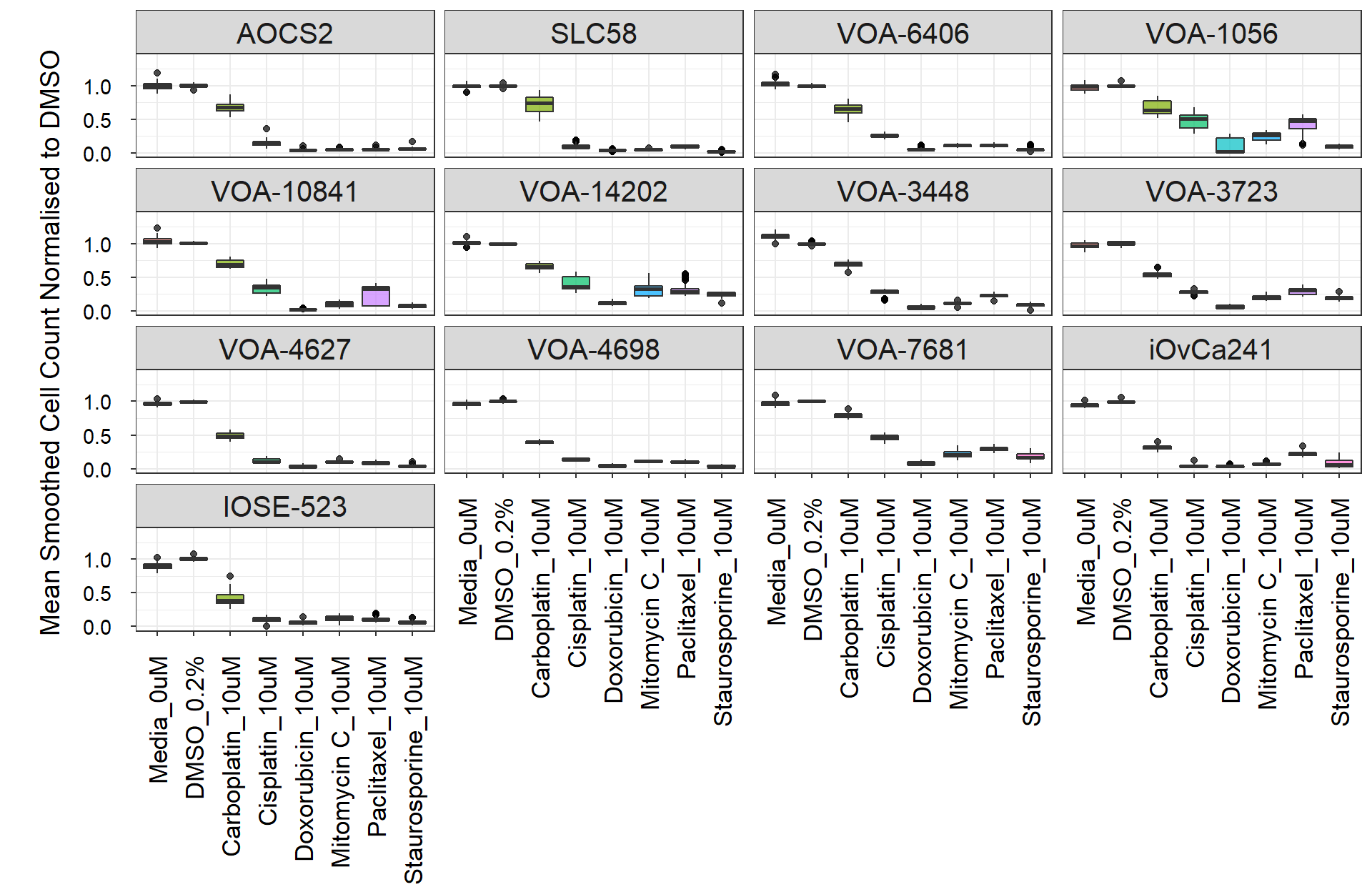
#dev.off()Hit identification
Reduced compound list
After the first two screens were performed, the FDA compound list was reduced down to compounds in clinical development for subsequent screens. Hit selection was performed on the final list of 3382 compounds screened across all cell lines (the entire Kinase and Epigenetics libraries and the FDA clinical development sub-library).
final_comp_list <- read_csv("data/CA_OpenAccess_FDA_MCE_clinical_dev_sublibrary_2022.csv") %>%
  pull(QCL_Sample_Number)

data_norm_smooth_filt <- data_norm_smooth %>%
  filter(Library %in% c("Epigenetics", "Kinase") | QCL_Sample_Number %in% c(final_comp_list))
Viability binning
Compounds were sorted into the following viability bins based on the normalised cell counts:
- High viability (> 1.15)
- Normal viability (0.8 <= 1.15)
- Moderate viability (0.5 <= 0.8)
- Low viability (<= 0.5)
data_binned <- data_norm_smooth_filt %>%
  filter(Description == "Sample") %>%
  mutate(Viability_Bin = ifelse(Count_Cells_Norm_fit > 1.15, "High",
          ifelse((Count_Cells_Norm_fit > 0.8 & Count_Cells_Norm_fit <= 1.15), "Normal",
          ifelse((Count_Cells_Norm_fit > 0.5 & Count_Cells_Norm_fit <= 0.8), "Moderate",
          ifelse(Count_Cells_Norm_fit <= 0.5, "Low", "NA")))))
Robust Z-Scoring
The normalised values were Robust Z-Scored to the median of all of the test compounds (at 0.1 and 1uM) in order to assess the relative strength of each compound (each cell line was calculated separately). This method can be used to select the strongest and most robust hits from a large dataset. Z-Scores of <= -2 or >= 2 are considered to be significant, but this value must be viewed in combination with the fold change.
# remove 10uM dose
data_zscored <- data_binned %>%
  filter(!Concentration == 10) %>%
  group_by(Cell_Line) %>%
  mutate(Robust_ZScore = (Count_Cells_Norm_fit - median(Count_Cells_Norm_fit))/mad(Count_Cells_Norm_fit)) %>%
  mutate_at(17, round, 2)

#write_csv(data_zscored, paste0("output/data_records/", prefix, "_Data_Record_3.csv"))
Waterfall plots
Robust Z-Scores for all of the test compounds are displayed below.
The number of hits (unique QCL_Sample_Numbers) and corresponding fold
change (FC) at Z-Score a cut-off of 2 are printed below the plot.
# prepare the data
data_zscored_plot <- ungroup(data_zscored) %>%
  unite(Conc, c(Concentration, Units), sep = "") %>%
  unite(Treatment, c(Compound_Name, Conc), remove = FALSE) %>%
  mutate(Status = ifelse(Robust_ZScore >= 2, "Viability Increase Hits",
                  ifelse(Robust_ZScore <= -2, "Viability Decrease Hits", "Non-Significant"))) %>%
  arrange(Cell_Line, Robust_ZScore) %>%
  group_by(Cell_Line) %>%
  mutate(Index = 1:n())

# set order of status for plotting
stat_order <- c("Viability Increase Hits", "Viability Decrease Hits", "Non-Significant")
data_zscored_plot$Status <- factor(data_zscored_plot$Status, levels = stat_order)

# set order of cell lines for plotting
data_zscored_plot$Cell_Line <- factor(data_zscored_plot$Cell_Line, levels = cell_order)

# create dot plot
snake_plot1 <- data_zscored_plot %>%
  filter(Cell_Line %in% c("AOCS2", "SLC58", "VOA-6406", "VOA-1056", "VOA-10841", "VOA-14202")) %>%
  ggplot(., aes(x = Index,
                y = Robust_ZScore,
                label = Treatment)) +
  geom_point(aes(colour = Status),
                 alpha = 0.8, size = 1.6) +
  facet_grid(Cell_Line~Conc) +
  geom_hline(aes(yintercept = -2), linetype = "dotted", size = 0.3) +
  geom_hline(aes(yintercept = 2), linetype = "dotted", size = 0.3) +
  labs(x = "Rank",
       y = "Robust Z-Score") +
  scale_y_continuous(breaks = seq(-12, 10, by = 2), limits=c(-12,10)) +
  theme_bw() +
  theme(axis.title.y = element_text(margin = margin(t = 0, r = 10, b = 0, l = 10), size = 12),
        axis.title.x = element_text(margin = margin(t = 10, r = 0, b = 10, l = 0), size = 12),
        axis.text.x = element_blank(),
        axis.ticks.x = element_blank(),
        axis.text.y = element_text(colour = "black"),
        plot.title = element_text(margin = margin(t = 10, r = 0, b = 5, l = 0), size = 14),
        plot.margin = margin(t = 10, r = 5, b = 5, l = 10),
        strip.text = element_text(size = 12),
        legend.title = element_blank(),
        legend.text = element_text(size = 13)) +
  scale_colour_manual(values = c("#bc3754", "#2a788e", "grey61"), drop = TRUE)

# create dot plot
snake_plot2 <- data_zscored_plot %>%
  filter(Cell_Line %in% c("VOA-3448", "VOA-3723", "VOA-4627", "VOA-4698", "VOA-7681", "iOvCa241")) %>%
  ggplot(., aes(x = Index,
                y = Robust_ZScore,
                label = Treatment)) +
  geom_point(aes(colour = Status),
                 alpha = 0.8, size = 1.6) +
  facet_grid(Cell_Line~Conc) +
  geom_hline(aes(yintercept = -2), linetype = "dotted", size = 0.3) +
  geom_hline(aes(yintercept = 2), linetype = "dotted", size = 0.3) +
  labs(x = "Rank",
       y = "Robust Z-Score") +
  scale_y_continuous(breaks = seq(-12, 10, by = 2), limits=c(-12,10)) +
  theme_bw() +
  theme(axis.title.y = element_blank(),
        axis.title.x = element_text(margin = margin(t = 10, r = 0, b = 10, l = 0), size = 12),
        axis.text.x = element_blank(),
        axis.ticks.x = element_blank(),
        axis.text.y = element_text(colour = "black"),
        plot.title = element_text(margin = margin(t = 10, r = 0, b = 5, l = 0), size = 14),
        plot.margin = margin(t = 10, r = 5, b = 5, l = 5),
        strip.text = element_text(size = 12),
        legend.title = element_blank(),
        legend.text = element_text(size = 13)) +
  scale_colour_manual(values = c("#bc3754", "#2a788e", "grey61"), drop = TRUE)

# create dot plot
snake_plot3 <- data_zscored_plot %>%
  filter(Cell_Line == "IOSE-523") %>%
  ggplot(., aes(x = Index,
                y = Robust_ZScore,
                label = Treatment)) +
  geom_point(aes(colour = Status),
                 alpha = 0.8, size = 1.6) +
  facet_grid(Cell_Line~Conc) +
  geom_hline(aes(yintercept = -2), linetype = "dotted", size = 0.3) +
  geom_hline(aes(yintercept = 2), linetype = "dotted", size = 0.3) +
  labs(x = "Rank",
       y = "Robust Z-Score") +
  scale_y_continuous(breaks = seq(-12, 10, by = 2), limits=c(-12,10)) +
  theme_bw() +
  theme(axis.title.y = element_blank(),
        axis.title.x = element_text(margin = margin(t = 10, r = 0, b = 10, l = 0), size = 12),
        axis.text.x = element_blank(),
        axis.ticks.x = element_blank(),
        axis.text.y = element_text(colour = "black"),
        plot.title = element_text(margin = margin(t = 10, r = 0, b = 5, l = 0), size = 14),
        plot.margin = margin(t = 10, r = 10, b = 5, l = 5),
        strip.text = element_text(size = 12),
        legend.title = element_blank(),
        legend.text = element_text(size = 13)) +
  scale_colour_manual(values = c("#bc3754", "#2a788e", "grey61"), drop = TRUE)


design <- "
  123
  12#
  12#
  12#
  12#
  12#
"

#tiff(paste0("output/hit_figs/", prefix, "_WaterfallPlot.tiff"), width = 6200, height = 5000, units = "px", res = 400)
snake_plot1 + snake_plot2 + snake_plot3 + plot_layout(guides = "collect", ncol = 3, design = design)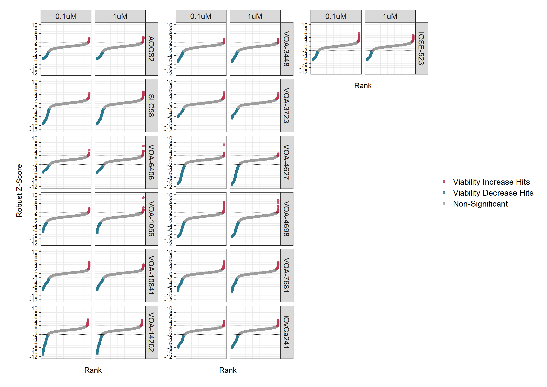
#dev.off()total_comps <- n_distinct(data_zscored$QCL_Sample_Number)
hit_count_summary <- data_zscored %>%
unite(Conc, c(Concentration, Units), sep = "") %>%
mutate(ZScore_Bin = ifelse(Robust_ZScore >= 2, ">= 2",
ifelse(Robust_ZScore <= -2, "<= -2",
"NonSig"))) %>%
filter(!ZScore_Bin == "NonSig") %>%
group_by(Cell_Line, Conc, ZScore_Bin) %>%
summarise(Equivalent_FC_max = max(Count_Cells_Norm_fit),
Equivalent_FC_min = min(Count_Cells_Norm_fit),
Hit_Count = n_distinct(QCL_Sample_Number)) %>%
pivot_longer(c(Equivalent_FC_max, Equivalent_FC_min),
names_to = "Direction", values_to = "Equivalent_FC") %>%
filter(c(grepl('<', ZScore_Bin) & Direction == "Equivalent_FC_max") |
c(grepl('>', ZScore_Bin) & Direction == "Equivalent_FC_min")) %>%
mutate(ZScore_Bin = factor(ZScore_Bin, levels = c(">= 2", "<= -2")),
Cell_Line = factor(Cell_Line, levels = cell_order),
Hit_Rate = (Hit_Count / total_comps)*100) %>%
select(Cell_Line, Conc, ZScore_Bin, Equivalent_FC, Hit_Count, '%Hit_Rate' = Hit_Rate) %>%
arrange(Cell_Line, Conc, ZScore_Bin) %>%
mutate_at(6, round, 2)
#write_csv(hit_count_summary, paste0("output/", prefix, "_Hit_Counts.csv"))
# display the data in a table
datatable(hit_count_summary, extensions = c('Buttons', 'Scroller', "FixedColumns"), rownames = FALSE,
options = list(
dom = 'Blfrt',
columnDefs = list(list(className = 'dt-center',targets="_all")),
lengthMenu = list(c(5, -1), c('5', 'All')),
pageLength = 5,
buttons = list(list(extend = 'csv',
filename = gsub(" ", "", paste(prefix, "_Hit_Rate"))),
list(extend = 'excel',
filename = gsub(" ", "", paste(prefix, "_Hit_Rate")), title = NULL)),
searching = FALSE,
scrollX = TRUE,
fixedColumns = list(leftColumns = 3))) Hit validation
Secondary screen data was read into R studio and dose-response plots were generated for each compound.
data_val <- read_csv("data/validation_data/KP_PMC185_Viability_data.csv") %>%
  select(Barcode, Media, Cell_Line, VCFG_Plate_ID, Replicate, WellID, Description, MedChem_Compound_Name = Compound_Name, CA_Compound_Name, Concentration, Units, contains("Count_Cells")) %>%
  rbind(., read_csv("data/validation_data/KP_PMC184_Viability_data.csv")) %>%
  filter(c(Media == "Standard" & !Description %in% c("Skipped", "Excluded"))) %>%
  select(Barcode, Cell_Line, VCFG_Plate_ID, Replicate, WellID, Description, CA_Compound_Name, MedChem_Compound_Name, Concentration, Units, contains("Count_Cells")) %>%
  mutate_at(12:13, round, 2)

write_csv(data_val, paste0("output/data_records/", prefix, "_Data_Record_4.csv"))
val_comps <- read_csv("data/KP_val_comps.csv") %>%
select(MedChem_Compound_Name) %>%
pull()
perwell_plot <- data_val %>%
filter(MedChem_Compound_Name %in% val_comps) %>%
mutate(MedChem_Compound_Name = ifelse(MedChem_Compound_Name == "Methyl aminolevulinate (hydrochloride)", "Methyl aminolevulinate", MedChem_Compound_Name)) %>%
filter(c(Description == "Sample" | c(MedChem_Compound_Name == "MitomycinC" & !is.na(CA_Compound_Name))) & Concentration %in% c(10, 1, 0.1, 15.977000, 1.576000, 0.155300))
perwell_plot$Cell_Line <- factor(perwell_plot$Cell_Line, levels = c("iOvCa241", "VOA-10841", "VOA-3448", "VOA-4698"))
p1 <- perwell_plot %>%
ggplot(.,aes(x = Concentration,
y = Count_Cells_Norm_fit,
colour = factor(Cell_Line),
group = Cell_Line)) +
geom_point(alpha = 0.8, size = 1.9) +
geom_hline(aes(yintercept = 0.5), linetype = "dotted", size = 0.4) +
geom_hline(aes(yintercept = 1.0), linetype = "dotted", size = 0.4) +
geom_hline(aes(yintercept = 1.5), linetype = "dotted", size = 0.4) +
geom_smooth(method = drm, method.args = list(fct = L.4()), se = FALSE, size = 2.2) +
facet_wrap(~MedChem_Compound_Name, ncol = 6) +
labs(x = "Concentration (log10)",
y = "Smoothed Cell Count Normalised to DMSO") +
ylim(0, 1.75) +
scale_x_continuous(trans='log10') +
theme_bw() +
theme(axis.title.x = element_text(margin = margin(t = 10, r = 10, b = 20, l = 20), size = 26),
axis.title.y = element_text(margin = margin(t = 0, r = 10, b = 0, l = 20), size = 26),
axis.text.x = element_text(angle = 45, colour = "black", size = 20, hjust = 1),
axis.text.y = element_text(colour = "black", size = 20),
strip.text = element_text(size = 15, face = "bold"),
legend.text = element_text(size = 26),
legend.title = element_blank(),
plot.subtitle = element_text(size = 27, face = "bold"),
plot.margin = margin(t = 20, r = 30, b = 0, l = 10))
tiff(paste0("output/val_figs/", prefix, "_Validation_DoseResponse_20240315.tiff"), units="in", width=25, height=35, res=300)
p1
dev.off()
jpeg(paste0("output/val_figs/", prefix, "_Validation_DoseResponse_20240315.jpeg"), units="in", width=25, height=35, res=300, quality = 100)
p1
dev.off()
# save the plot as a PDF
# pdf(paste0("output/val_figs/", prefix, "_Validation_DoseResponse_20240315.pdf"), width = 32, height = 50)
# p1
# dev.off()
Analysed by Karla Cowley
Victorian Centre for Functional Genomics
sessionInfo()R version 4.3.1 (2023-06-16 ucrt)
Platform: x86_64-w64-mingw32/x64 (64-bit)
Running under: Windows 10 x64 (build 19045)
Matrix products: default
locale:
[1] LC_COLLATE=English_Australia.utf8 LC_CTYPE=English_Australia.utf8
[3] LC_MONETARY=English_Australia.utf8 LC_NUMERIC=C
[5] LC_TIME=English_Australia.utf8
time zone: Australia/Sydney
tzcode source: internal
attached base packages:
[1] stats graphics grDevices utils datasets methods base
other attached packages:
[1] viridis_0.6.5 viridisLite_0.4.2 lubridate_1.9.3 forcats_1.0.0
[5] stringr_1.5.1 dplyr_1.1.3 purrr_1.0.2 readr_2.1.5
[9] tidyr_1.3.0 tibble_3.2.1 ggplot2_3.3.0 tidyverse_2.0.0
[13] patchwork_1.2.0 reshape2_1.4.4 drc_3.0-1 MASS_7.3-60
[17] DT_0.32 data.table_1.14.8 workflowr_1.7.1
loaded via a namespace (and not attached):
[1] tidyselect_1.2.1 farver_2.1.1 fastmap_1.1.1 TH.data_1.1-2
[5] promises_1.2.1 digest_0.6.33 timechange_0.3.0 lifecycle_1.0.4
[9] ellipsis_0.3.2 survival_3.5-5 processx_3.8.2 magrittr_2.0.3
[13] compiler_4.3.1 rlang_1.1.1 sass_0.4.8 tools_4.3.1
[17] plotrix_3.8-4 utf8_1.2.3 yaml_2.3.7 knitr_1.45
[21] labeling_0.4.3 htmlwidgets_1.6.4 bit_4.0.5 plyr_1.8.9
[25] multcomp_1.4-25 abind_1.4-5 withr_3.0.0 grid_4.3.1
[29] fansi_1.0.4 git2r_0.32.0 colorspace_2.1-0 scales_1.3.0
[33] gtools_3.9.5 cli_3.6.1 mvtnorm_1.2-4 crayon_1.5.2
[37] rmarkdown_2.26 generics_0.1.3 rstudioapi_0.15.0 httr_1.4.7
[41] tzdb_0.4.0 cachem_1.0.8 splines_4.3.1 parallel_4.3.1
[45] vctrs_0.6.3 Matrix_1.6-5 sandwich_3.1-0 jsonlite_1.8.7
[49] carData_3.0-5 car_3.1-2 callr_3.7.5 hms_1.1.3
[53] bit64_4.0.5 crosstalk_1.2.1 jquerylib_0.1.4 glue_1.6.2
[57] codetools_0.2-19 ps_1.7.5 stringi_1.7.12 gtable_0.3.4
[61] later_1.3.1 munsell_0.5.0 pillar_1.9.0 htmltools_0.5.7
[65] R6_2.5.1 rprojroot_2.0.4 vroom_1.6.5 evaluate_0.23
[69] lattice_0.21-8 highr_0.10 httpuv_1.6.11 bslib_0.6.1
[73] Rcpp_1.0.11 gridExtra_2.3 whisker_0.4.1 xfun_0.40
[77] fs_1.6.3 zoo_1.8-12 getPass_0.2-2 pkgconfig_2.0.3