Last updated: 2025-03-24

Checks: 6 1

Knit directory: McConville_Lab_Microbiome_PMC255A/

This reproducible R Markdown analysis was created with workflowr (version 1.7.1). The Checks tab describes the reproducibility checks that were applied when the results were created. The Past versions tab lists the development history.

R Markdown file: uncommitted changes

The R Markdown is untracked by Git. To know which version of the R Markdown file created these results, you’ll want to first commit it to the Git repo. If you’re still working on the analysis, you can ignore this warning. When you’re finished, you can run wflow_publish to commit the R Markdown file and build the HTML.

Environment: empty

Great job! The global environment was empty. Objects defined in the global environment can affect the analysis in your R Markdown file in unknown ways. For reproduciblity it’s best to always run the code in an empty environment.

Seed: set.seed(20250117)

The command set.seed(20250117) was run prior to running the code in the R Markdown file. Setting a seed ensures that any results that rely on randomness, e.g. subsampling or permutations, are reproducible.

Session information: recorded

Great job! Recording the operating system, R version, and package versions is critical for reproducibility.

Cache: none

Nice! There were no cached chunks for this analysis, so you can be confident that you successfully produced the results during this run.

File paths: relative

Great job! Using relative paths to the files within your workflowr project makes it easier to run your code on other machines.

Repository version: 3a65c0b

Great! You are using Git for version control. Tracking code development and connecting the code version to the results is critical for reproducibility.

The results in this page were generated with repository version 3a65c0b. See the Past versions tab to see a history of the changes made to the R Markdown and HTML files.

Note that you need to be careful to ensure that all relevant files for the analysis have been committed to Git prior to generating the results (you can use wflow_publish or wflow_git_commit). workflowr only checks the R Markdown file, but you know if there are other scripts or data files that it depends on. Below is the status of the Git repository when the results were generated:


Ignored files:
    Ignored:    .Rhistory
    Ignored:    .Rproj.user/
    Ignored:    data/raw_data/

Untracked files:
    Untracked:  analysis/PMC255A_ScreenQC_v4.Rmd
    Untracked:  analysis/prelim/

Unstaged changes:
    Modified:   analysis/PMC255A_ScreenComparison.Rmd
    Deleted:    analysis/PMC255A_ScreenQC_v3.Rmd
    Modified:   analysis/_site.yml

Note that any generated files, e.g. HTML, png, CSS, etc., are not included in this status report because it is ok for generated content to have uncommitted changes.

There are no past versions. Publish this analysis with wflow_publish() to start tracking its development.

Aim

To examine the polarisation potential of BDBM cells from M0 to M1 or M2 in the presence of compounds and different concentrations of polarisation activator.

Researcher

Ada Koo, McConville Lab, Bedoui Lab

Readout

Image analysis of BMDM cells stained with DAPI, ARG, INOS, and BODIPY (CX7 Pro LZR, 9 fields0 @ 20x)

Image analysis software

CellProfiler 4.1.3

Required R packages

data.table, DT, reshape2, tidyverse, viridis, patchwork

# load the required packages
library(data.table)
library(readxl)
library(DT)
library(reshape2)
library(viridis)
library(patchwork)
library(tidyverse)
library(magick)

# fix ggplotly axis labels
layout_ggplotly <- function(gg, x = -0.02, y = -0.08){
  # The 1 and 2 goes into the list that contains the options for the x and y axis labels respectively
  gg[['x']][['layout']][['annotations']][[1]][['y']] <- x
  gg[['x']][['layout']][['annotations']][[2]][['x']] <- y
  gg
}

# set the file prefix
prefix <- "KW_PMC255A"

# turn off scientific notation
options(scipen=999)

Screen details

Screen dates (yyyy-mm-dd)

2024-12-04

Cell lines

BMDM M0

Conditions

unstimulated (Unstim_M0)
5 ng/mL IL4 + 5 ng/mL IL13 (Lo_M2)
10 ng/mL IL4 + 10 ng/mL IL13 (Hi_M2)
3 ng/mL IFNg + 3 ng/mL LPS (Lo_M1)
25 ng/mL IFNg + 25 ng/mL LPS (Hi_M1)
25 ng/mL IFNg (Potential_M1)

Screen outline

Library: Custom MCE library
Library plates: 4
Cell plates per library plate: 24

Controls

Per well data is normalised to Stimulated DMSO on a per plate basis.

Known technical issues

None.

Plate layout

get_image_dimensions <- function(path) {
  img_info <- magick::image_info(magick::image_read(path))
  setNames(c(img_info$width, img_info$height), c("Width", "Height"))
}

# Example usage
path <- file.path("data", paste0(prefix, "_platemap.png"))
img_dims <- get_image_dimensions(path)

# Generate the HTML image with scaled dimensions
htmltools::img(
  src = knitr::image_uri(path),
  style = sprintf("height:%.0fpx;width:%.0fpx;", img_dims["Height"] / 2, img_dims["Width"] / 2)
)

Data cleaning

The raw data was read into R Studio.

data_raw_obj <- list.files(path = paste0("data/raw_data/PerObject/"), # list all .csv files
                              pattern = "*.csv", 
                              full.names = T) %>%
  set_names(nm = basename(.)) %>%  
  map_dfr(., fread, .id = "FileName") %>% # Add file name as a column
  mutate(FileName = tools::file_path_sans_ext(FileName)) %>%  # remove .csv extensions
  as.data.frame() %>% 
  mutate(Barcode = FileName,
         Barcode = gsub("PerObject_|_Cytoplasm", "", Barcode),
         Barcode = gsub("Rep", "Plate", Barcode),
         Barcode = gsub("Unsure", "Potential", Barcode)) %>% 
  select(Barcode,
         PlateID = matches("^Metadata_PlateID", ignore.case = FALSE)[1],
         WellID = matches("^Metadata_WellID", ignore.case = FALSE)[1],
         Field = matches("^Metadata_Field", ignore.case = FALSE)[1],
         Bodipy_spots_count = Children_BODIPY_spots_Count,
         Intensity_IntegratedIntensity_BODIPY = matches("^Intensity_IntegratedIntensity_BODIPY", ignore.case = FALSE)[1],
         Intensity_MeanIntensity_BODIPY = matches("^Intensity_MeanIntensity_BODIPY", ignore.case = FALSE)[1],
         Intensity_StdIntensity_BODIPY = matches("^Intensity_StdIntensity_BODIPY", ignore.case = FALSE)[1],
         contains(c("ARG", "INOS"))) 

# data_raw_obj %>%  #H01
#   filter(grepl("A17", WellID) & grepl("Unstim_M0_Plate4", Barcode)) %>%
#   select(Field, contains(c("MeanIntensity"))) %>% 
#   group_by(Field) %>% 
#   summarise(across(contains(c("MeanIntensity")), lst(sum)))

Data processing

## Annotation

Well annotations were added to the Per Object data.

# read in annotation files
plate_info <- read_csv(paste0("data/KW_PMC255A_barcodes.csv"), show_col_types = FALSE) 

annotation <- read_csv(paste0("data/annot/", prefix, "_annotation.csv"), show_col_types = FALSE) 

# annotate data
data_annot_obj <- data_raw_obj %>%
  left_join(plate_info, ., by = c("Barcode", "PlateID")) %>% 
  left_join(annotation, .,  by = c("WellID", "VCFG_Plate_ID" = "Replicate")) %>% 
  select(-PlateID2) %>% 
  # fix concentration, units and labels for each plate
  mutate(Concentration = case_when(Compound_Name == "IL4+IL13" ~ 50,
                                   Compound_Name == "LPS+INFg" ~ 50,
                                   TRUE ~ Concentration),
         Units = case_when(grepl("IL4\\+IL13|LPS\\+INFg", Compound_Name) ~ "ng/mL",
                                   TRUE ~ Units),
         Stimulation = case_when(grepl("01", WellID) ~ "Unstimulated", TRUE ~ "Stimulated"))

# write out image annot file
write_excel_csv(data_annot_obj, "output/data_annot_obj.csv")

# clean up annotation files
annotation <- read_csv(paste0("data/annot/", prefix, "_annotation.csv"), show_col_types = FALSE) 
plate_info <- read_csv(paste0("data/KW_PMC255A_barcodes.csv"), show_col_types = FALSE) 

# replace non-alphanumeric characters in compound names
library(tidyverse)
library(data.table)
library(stringi)
 
annot_clean <- annotation %>% 
  mutate(Compound_Name_Clean = gsub(" ", "_", Compound_Name), 
         Compound_Name_Clean = stri_trans_general(Compound_Name_Clean, "Latin-ASCII"),      
         Compound_Name_Clean = gsub("α", "alpha", Compound_Name_Clean),
         Compound_Name_Clean = gsub("β", "beta", Compound_Name_Clean),
         Compound_Name_Clean = gsub("γ", "gamma", Compound_Name_Clean),
         Compound_Name_Clean = gsub("κ", "kappa", Compound_Name_Clean),
         Compound_Name_Clean = gsub("Δ|δ", "delta", Compound_Name_Clean),
         Compound_Name_Clean = gsub("Θ|θ", "theta", Compound_Name_Clean),
         Compound_Name_Clean = gsub("ι", "iota", Compound_Name_Clean),
         Compound_Name_Clean = gsub("Λ|λ", "lambda", Compound_Name_Clean),
         Compound_Name_Clean = gsub("μ", "mu", Compound_Name_Clean),
         Compound_Name_Clean = gsub("ν", "nu", Compound_Name_Clean),
         Compound_Name_Clean = gsub("Σ|σ", "sigma", Compound_Name_Clean),
         Compound_Name_Clean = gsub("Φ|φ", "phi", Compound_Name_Clean),
         Compound_Name_Clean = gsub("Π|π", "pi", Compound_Name_Clean),
         Compound_Name_Clean = gsub("Ψ|ψ", "psi", Compound_Name_Clean),
         Compound_Name_Clean = gsub("Ω|ω", "omega", Compound_Name_Clean),
         Compound_Name_Clean = gsub("ρ", "rho", Compound_Name_Clean),
         Compound_Name_Clean = gsub("[^[:alnum:]]", "", Compound_Name_Clean))

# Find rows containing non-English characters in the text_column
non_english_rows <- grep("[^[:alnum:]_-]", annot_clean$Compound_ID_Clean, value = FALSE)
 
# Subset dataframe to rows with non-English characters
df_non_english <- annot_clean[non_english_rows, ]
 
View(df_non_english)

annot_clean_complete <- annot_clean %>% 
  inner_join(., plate_info, by = c("VCFG_Plate_ID" = "Replicate")) %>% 
  select(PlateID, VCFG_Plate_ID, Barcode, WellID, QCL_Sample_Number, Compound_Name, Compound_Name_Clean, Concentration, Units) %>% 
  distinct()
 
write_csv(annot_clean_complete, paste0("output/", prefix, "_image_annotation.csv"))

data_annot_obj <- read_csv("output/data_annot_obj.csv")

Thresholding

Histograms below shows the count of percentage positive cells for ARG and INOS staining based on the negative control (Unstimulated DMSO). Dotted red line indicates the cut off used for thresholding positive percentage cells in the Unstimulated DMSO wells across all plates.

Thresholds for percentage positive cells were set globally based on the following limits:
* ARG positive threshold (MeanIntensity >= mean_intensity_ARG of DMSO + 1.5 x std_dev_ARG)
* INOS positive threshold (MeanIntensity >= mean_intensity_INOS of DMSO + 1.25 x std_dev_INOS)
* BODIPY positive (>= 2 spot count)

# create function to generate density plot
gendensityplot <-  function(vars, limits){

  # for labelling purposes
  data_annot_obj$VCFG_Plate_ID <- paste("VCFG_Plate_ID:", data_annot_obj$VCFG_Plate_ID)
    
  # filter data and add polarity description
  data_annot_obj_filt <- data_annot_obj %>%
    filter((!grepl("Media", Compound_Name)) & grepl("01", WellID)) 

  # calculate the median and standard deviation per plate
  stats_perplate <- ungroup(data_annot_obj_filt) %>% 
    filter(Compound_Name == "DMSO") %>% # use untreated instead of treated DMSO
    group_by(VCFG_Plate_ID) %>% 
    summarise(
      mean_intensity = mean(.data[[vars]], na.rm = TRUE),
      std_dev = sd(.data[[vars]], na.rm = TRUE),
      threshold_low = mean_intensity - limits * std_dev,
      threshold_high = mean_intensity + ifelse(VCFG_Plate_ID == "Plate4", 0.75, limits) * std_dev,
      lim = limits)

  data_annot_obj$VCFG_Plate_ID <- paste("VCFG_Plate_ID:", data_annot_obj$VCFG_Plate_ID)
  # plot density plot
  ggplot(data_annot_obj_filt, aes(x = .data[[vars]], fill = Compound_Name, color = Compound_Name)) +
    geom_density(alpha = 0.4) +
    geom_vline(data = stats_perplate, aes(xintercept = threshold_high), color = "black", linetype = "dashed", size = 0.5) +
  facet_wrap(~VCFG_Plate_ID+Compound_Name, scales = "free", ncol = 6) +
    labs(title = vars, x = vars,  y = "Density") +
    theme_bw() +
    theme(
      plot.title = element_text(size = 14),
      axis.text.y = element_text(size = 11),
      axis.text.x = element_text(size = 11),
      legend.title = element_text(size = 12),
      legend.text = element_text(size = 11))
}

# test different limits to determine final threshold cut off for percentage positive cells
(gendensityplot("Intensity_MeanIntensity_ARG", 1.5) /
gendensityplot("Intensity_MeanIntensity_INOS", 1.25)) /
  plot_layout(guides = "collect")

# create function to generate density plot
gendensityplot <-  function(vars, limits){

  # filter data and add polarity description
  data_annot_obj_filt <- data_annot_obj %>%
    filter((!grepl("Media", Compound_Name)) & grepl("01", WellID)) 

  # calculate the median and standard deviation per plate
  stats_perplate <- ungroup(data_annot_obj_filt) %>% 
    filter(Compound_Name == "DMSO") %>% # use untreated instead of treated DMSO
    group_by(Barcode) %>% 
    summarise(
      mean_intensity = mean(.data[[vars]], na.rm = TRUE),
      std_dev = sd(.data[[vars]], na.rm = TRUE),
      threshold_low = mean_intensity - limits * std_dev,
      threshold_high = mean_intensity + limits * std_dev,
      lim = limits)

  # plot density plot
  ggplot(data_annot_obj_filt, aes(x = .data[[vars]], fill = Compound_Name, color = Compound_Name)) +
    geom_density(alpha = 0.4) +
    geom_vline(data = stats_perplate, aes(xintercept = threshold_high), color = "black", linetype = "dashed", size = 0.5) +
  facet_wrap(~Barcode+Compound_Name, scales = "free", ncol = 12) +
    labs(title = vars, x = vars,  y = "Density") +
    theme_bw() +
    theme(
      legend.position = 'top',
      plot.title = element_text(size = 14),
      axis.text.y = element_text(size = 11),
      axis.text.x = element_text(size = 11),
      legend.title = element_text(size = 12),
      legend.text = element_text(size = 11))
}

# test different limits to determine final threshold cut off for percentage positive cells

plot1 <- gendensityplot("Intensity_MeanIntensity_ARG", 1.5)
plot2 <- gendensityplot("Intensity_MeanIntensity_INOS", 1.25)
# save the plot as a PDF
pdf(paste0("output/", prefix, "_DensityPlots.pdf"), width = 25, height = 13)
print(plot1)
print(plot2)
dev.off()

Aggregation

The per-cell data was aggregated into per-well data (total cell counts and % positive cells in each channel).

# generate limits
neg_limits <- data_annot_obj %>% 
  group_by(Barcode) %>% 
  filter(grepl("01", WellID) & Compound_Name == "DMSO") %>% 
  summarise(arg_pos_limit = (mean(Intensity_MeanIntensity_ARG) + (1.5*sd(Intensity_MeanIntensity_ARG))),
            inos_pos_limit = (mean(Intensity_MeanIntensity_INOS) + (1.25*sd(Intensity_MeanIntensity_INOS))),
            bodipy_pos_limit = 2)

data_perwell <- data_annot_obj %>% 
  left_join(., neg_limits, by = c("Barcode")) %>% 
  mutate(
    ARG_label = case_when(
      Intensity_MeanIntensity_ARG >= arg_pos_limit ~ "ARG_positive", TRUE ~ "ARG_negative"),
    INOS_label = case_when(
      Intensity_MeanIntensity_INOS >= inos_pos_limit ~ "INOS_positive", TRUE ~ "INOS_negative"),
    `INOS+BODIPY_label` = case_when((Intensity_MeanIntensity_INOS >= inos_pos_limit & Bodipy_spots_count >=
                                      bodipy_pos_limit) ~ "INOS+BODIPY_positive", TRUE ~ "INOS+BODIPY_negative"),
    `INOS-BODIPY_label` = case_when((Intensity_MeanIntensity_INOS >= inos_pos_limit & Bodipy_spots_count <
                                      bodipy_pos_limit) ~ "INOS-BODIPY_positive", TRUE ~ "INOS-BODIPY_negative"),
    `BODIPY_label` = case_when(Bodipy_spots_count >=
                                      bodipy_pos_limit ~ "BODIPY_positive", TRUE ~ "BODIPY_negative")) %>%
    mutate(Condition_Name = case_when(grepl("Unstim_M0", Barcode) ~ "Unstimulated",
                                     grepl("Potential_M1", Barcode) ~ "25 ng/mL INFg",
                                     grepl("Lo_M1", Barcode) ~ "3 ng/mL INFg + 3 ng/mL LPS",
                                     grepl("Hi_M1", Barcode) ~ "25 ng/mL INFg + 25 ng/mL LPS", 
                                     grepl("Lo_M2", Barcode) ~ "5 ng/mL IL4 + 5 ng/mL IL13",
                                     grepl("Hi_M2", Barcode) ~ "10 ng/mL IL4 + 10 ng/mL IL13"),
         Phenotype = case_when(grepl("Unstim_M0", Barcode) ~ "M0",
                                     grepl("Potential_M1", Barcode) ~ "M1",
                                     grepl("Lo_M1", Barcode) ~ "M1",
                                     grepl("Hi_M1", Barcode) ~ "M1", 
                                     grepl("Lo_M2", Barcode) ~ "M2",
                                     grepl("Hi_M2", Barcode) ~ "M2")) %>% 
  group_by(Barcode, PlateID, Description, WellID, QCL_Sample_Number, Compound_Name, Concentration, Units, VCFG_Plate_ID, Target, Pathway, Condition_Name, Phenotype, Stimulation) %>%
  summarise(Total_DAPI_Count = n(),
            # Total_MeanIntensity_ARG = mean(Intensity_MeanIntensity_ARG),
            # Total_MeanIntensity_INOS = mean(Intensity_MeanIntensity_INOS),
            # Total_StdIntensity_BODIPY = mean(Intensity_StdIntensity_BODIPY),
            Positive_Perc_ARG = sum(ARG_label == "ARG_positive")/n() * 100,
            Positive_Perc_INOS = sum(INOS_label == "INOS_positive")/n() * 100,
            `Positive_Perc_INOS+BODIPY` = sum(`INOS+BODIPY_label` == "INOS+BODIPY_positive")/n() * 100,
            `Positive_Perc_INOS-BODIPY` = sum(`INOS-BODIPY_label` == "INOS-BODIPY_positive")/n() * 100,
            `Positive_Perc_BODIPY` = sum(`BODIPY_label` == "BODIPY_positive")/n() * 100,
            `CellCount_BODIPY` =sum(`BODIPY_label` == "BODIPY_positive"),
            `SpotCount_BODIPY` = sum(`Bodipy_spots_count`),
            `MeanSpotCount_PerBODIPYPosCell` =  (`SpotCount_BODIPY`/`CellCount_BODIPY`),
            `MeanSpotCount_PerCell` = `SpotCount_BODIPY`/n()) %>% 
  select(-`CellCount_BODIPY`, -`SpotCount_BODIPY`)

# create a df for controls
data_perwell_controls <- data_perwell %>% 
  filter(grepl('Control', Description))

# write out the data
write_csv(data_perwell_controls, paste0("output/", prefix, "_data_perwell_controls.csv"))
write_csv(data_perwell, paste0("output/", prefix, "_data_perwell.csv"))

Normalisation

The raw values were normalised by fold changing to the median of the negative control (DMSO) wells within each plate.

# melt the dataframe
id <- colnames(data_perwell[1:14])
measure <- colnames(data_perwell[15:22])

data_perwell_melt <- data_perwell %>% 
  select(1:14, measure) %>% 
  melt(id.vars = id, measure.vars = measure) %>% 
  select(everything(), Raw = value, Feature = variable) %>% 
  arrange(Barcode, Feature, WellID) 

# normalise dataframe
data_norm_melt <- ungroup(data_perwell_melt) %>% 
  group_by(Barcode, Feature) %>%
  mutate(Raw = case_when(Raw == 0 ~ 0.00001, TRUE ~ Raw)) %>% 
  mutate(
    Compound_Name = case_when(grepl("01", WellID) ~ paste0(Compound_Name, "_Unstim"), TRUE ~ Compound_Name),
    NormToUnstimDMSO = Raw / median(Raw[Compound_Name == "DMSO_Unstim"], na.rm = TRUE),
    NormToStimDMSO = Raw / median(Raw[Compound_Name == "DMSO"], na.rm = TRUE)) %>% 
  left_join(., data_perwell_melt, by = c("Barcode", "PlateID", "Description", "WellID", "QCL_Sample_Number", "Compound_Name", "Concentration", "Units", "VCFG_Plate_ID", "Target", "Pathway", "Condition_Name", "Phenotype", "Stimulation", "Raw", "Feature")) %>% 
  ungroup() %>% 
  mutate(Description = case_when(grepl("Unstim_M0_Plate4", Barcode) & grepl("A17", WellID) & grepl("INOS", Feature) ~ "Excluded", TRUE ~ Description))

# unmelt the dataframe
data_norm <- data_norm_melt %>% 
  pivot_wider(names_from = Feature, values_from = c(Raw, NormToUnstimDMSO, NormToStimDMSO), names_glue = "{.value}_{Feature}")

write_excel_csv(data_norm, paste0("output/", prefix, "_data_norm.csv"))
write_excel_csv(data_norm_melt, paste0("output/", prefix, "_data_norm_melt.csv"))

# read in data
# data_norm_melt <- read.csv(paste0("output/", prefix, "_data_norm_melt.csv"))

Screen quality - DAPI Count

See the Screen quality section of the Methods page for a more information regarding what’s expected in terms of heat maps and screen and plate QC metrics, including %CVs and Z’ Factor values.

Heat maps

Comments: Clear edge effects affecting total cell count, however proportion of percentage positive ARG/INOS/BODIPY seem unaffected by edge effect. Overall pattern of death is consistent across plates.

# create a function to plot features
genheatmap <- function(feature){
  
  # filter the dataframe
  data_toplot <- data_norm_melt %>%
    filter(Feature == feature) %>% 
    arrange(Condition_Name) %>% 
    mutate(Raw = case_when(grepl("Empty", Description) ~ NA, TRUE ~ Raw)) %>% 
    mutate(Row = as.numeric(factor(substr(WellID, 1, 1), levels = LETTERS[1:16])),
    Column = as.numeric(substr(WellID, 2, 3)))
  
    # create feature heading
    cat("\n###", feature, "{.tabset .tabset-fade .tabset-pills} \n")

  # generate a list to plot
  plist <- list()
    
  # create for loop to plot per condition (or cell line)
  for (condition in unique(data_toplot$Condition_Name)){
    data_plot <- data_toplot %>%
      filter(Condition_Name == condition) #condition

    # create for loop to plot per plate
    for (i in unique(data_plot$Barcode)) {
    plot_df <- data_plot %>% 
      filter(Barcode == i)
      
    # Using geom tile to plot heat map
    plist[[i]] <- plot_df %>%
      ggplot(data = ., aes(x = Column, y = Row, fill = Raw)) +
      geom_tile(aes(linewidth = ifelse(grepl("Media", Compound_Name), "Media", "Non-Media")), 
                  colour = "black", width = 0.8, height = 0.8) +
      ggtitle(paste0(unique(plot_df$Barcode), ": \n", unique(plot_df$PlateID))) +
      scale_fill_gradient2(
        low = "blue", mid = "white", high = "red", na.value = "grey80",
        midpoint = median(plot_df$Raw, na.rm = TRUE),  # decide on the max,med,min, here it is from plot_df
        limits = c(min(plot_df$Raw, na.rm = TRUE), max(plot_df$Raw, na.rm = TRUE))) +
      scale_linewidth_manual(values = c("Media" = 0.65, "Non-Media" = 0.3), guide = "none") +
      scale_y_reverse(breaks = 1:16, labels = LETTERS[1:16]) +  # Y-axis for rows
      scale_x_continuous(breaks = 1:24, labels = sprintf("%02d", 1:24), position = "top") +  # X-axis for columns
      theme_bw() +
      theme(
          plot.title = element_text(size = 14),
          axis.text.x = element_text(size = 7),
          axis.text.y = element_text(size = 7),
          axis.title.x = element_blank(),
          axis.title.y = element_blank(),
          panel.grid = element_blank())
      }
  }
  cat("\n")
  #print all plots
  wrap_plots(plist) + plot_layout(ncol = 2) 
}

genheatmap("Total_DAPI_Count")

Total_DAPI_Count

Plate QC Metrics

Comments:
DMSO: %CVs are well within acceptable range except Hi_M2_Plate4 and Lo_M2_Plate4.
Unstim_DMSO: %CVs are well within acceptable range except Hi_M2_Plate3 and Unstim_M0_Plate4.
Media: %CVs are well within acceptable range except Hi_M2_Plate3.
Unstim_Media: %CVs are well within acceptable range except Lo_M1_Plate2 and Lo_M2_Plate2.
Staurosporine: %CVs are high, particularly for 10uM dose.
IL4+IL13: %CVs are within acceptable range except Lo_M2_Plate4.
IL4+IL13_Unstim: %CVs are within acceptable range except Hi_M2_Plate2, Lo_M2_Plate3.
LPS+INFg: %CVs are within acceptable range except Lo_M2_Plate4.
LPS+INFg_Unstim: %CVs are within acceptable range except Potential_M1_Plate2, Hi_M1_Plate1, Lo_M1_Plate4.
2DG, Antimycin, Itaconate: %CVs are high.

# filter down to control wells
ctrl_data <- ungroup(data_norm_melt) %>%
  filter(Description %in% c("Negative_Control", "Positive_Control")) %>% 
  unite(Conc, c(Concentration, Units), sep = "")

# Calculate summary statistics
screen_QC  <- ctrl_data %>% 
 group_by(Condition_Name, Compound_Name, Conc, Feature) %>%
  summarise_at(vars(Raw, NormToUnstimDMSO, NormToStimDMSO), lst(mean, sd), na.rm = TRUE) %>% 
  mutate(`NormToUnstimDMSO_%cv` = (`NormToUnstimDMSO_sd`/`NormToUnstimDMSO_mean`)*100) 
write_csv(screen_QC, paste0("output/", prefix, "_screen_QC.csv"))

# Calculate summary statistics
perplate_QC  <- ctrl_data %>% 
 group_by(Condition_Name, VCFG_Plate_ID, Compound_Name, Conc, Feature, Barcode) %>%
  summarise_at(vars(Raw, NormToUnstimDMSO, NormToStimDMSO), lst(mean, sd), na.rm = TRUE) %>% 
  mutate(`NormToUnstimDMSO_%cv` = (`NormToUnstimDMSO_sd`/`NormToUnstimDMSO_mean`)*100) 

write_csv(perplate_QC, paste0("output/", prefix, "_perplate_QC.csv"))

# create function to generate datatable
condition_list <- unique(perplate_QC$Condition_Name)
genplateqc <- function(feature){
    
    # print feature heading
    cat("\n### ", feature, "{.tabset .tabset-fade .tabset-pills}\n")
    
    # for loop to create condition plates
    for(condition in condition_list){
    cat("\n#### ", condition, "\n")
  
    perplate_QC_filt <- ungroup(perplate_QC) %>%
      filter(Feature == feature & Condition_Name == condition) %>%
      unite(Control, c(Compound_Name, Conc)) %>%
      mutate_if(is.numeric, round, 2) %>% 
      select(-Condition_Name, -Feature)
  
    # display the data in a table
    print(htmltools::tagList(datatable(
      perplate_QC_filt, extensions = c('Buttons', 'Scroller', "FixedColumns", 'ColReorder'), rownames = FALSE,
    options = list(
    dom = 'Blrtip',
    columnDefs = list(list(className = 'dt-center',targets="_all")),
    lengthMenu = list(c(5, -1), c("5", "All")),
    pageLength = 5,
    buttons = list(list(extend = 'csv',
                        filename = paste0(prefix, "_PerPlateQC_", feature, "_", condition)),
                   list(extend = 'excel',
                        filename = paste0(prefix, "_PerPlateQC_", feature, "_", condition), title = NULL)),
    searching = TRUE,
    scrollX = TRUE,
    fixedColumns = list(leftColumns = 2))) %>%
  formatStyle(c("NormToUnstimDMSO_%cv"), Color = styleInterval(24, c("Black", "red")), 
              fontWeight = styleInterval(24, c("bold", "bold")))))
    cat("\n")
    }
    cat("\n")
}
genplateqc("Total_DAPI_Count")

Total_DAPI_Count

10 ng/mL IL4 + 10 ng/mL IL13

25 ng/mL INFg

25 ng/mL INFg + 25 ng/mL LPS

3 ng/mL INFg + 3 ng/mL LPS

5 ng/mL IL4 + 5 ng/mL IL13

Unstimulated

Box plots

Comments:
DMSO - Small number of outliers, but values are very tight overall.

#create a list of features
feat_list <- unique(ctrl_data$Feature)
ctrl_data_plot <- ctrl_data %>%
  unite(Control, c(Compound_Name, Conc), remove = FALSE)

# set order of compounds for plotting
ctrl_order <- c("DMSO_Unstim_0.1%", "DMSO_0.1%", "Media_Unstim_0uM", "Media_0uM", 
                "INFg_Unstim_25ng/mL", "INFg_25ng/mL", 
                "IL4+IL13_50ng/mL", "IL4+IL13_Unstim_50ng/mL",
                "LPS+INFg_50ng/mL", "LPS+INFg_Unstim_50ng/mL",
                "2DG_0.5mM", "2DG_1mM", "2DG_2mM",
                "Antimycin_0.63uM", "Antimycin_1.25uM", "Antimycin_2.5uM",
                "Itaconate_0.5mM", "Itaconate_1mM", "Itaconate_2mM",
                "Staurosporine_0.1uM", "Staurosporine_1uM", "Staurosporine_10uM")

cond_labs_order <- c("Unstimulated", "25 ng/mL INFg",
                     "3 ng/mL INFg + 3 ng/mL LPS", "25 ng/mL INFg + 25 ng/mL LPS",
                     "5 ng/mL IL4 + 5 ng/mL IL13", "10 ng/mL IL4 + 10 ng/mL IL13")

ctrl_data_plot$Control <- factor(ctrl_data_plot$Control, levels = ctrl_order)
ctrl_data_plot$Condition_Name <- factor(ctrl_data_plot$Condition_Name, levels = cond_labs_order)

# create box plots with outliers
genboxplot <- function(compounds, vars){
  ctrl_data_plot %>%
  filter(grepl(compounds, Compound_Name) & Feature == vars) %>%
  ggplot(., aes(x = Control, 
                y = Raw,
                fill = Control)) +
  geom_boxplot(alpha = 0.7, notch = FALSE, outlier.colour = "black") +
  facet_grid(Condition_Name+Phenotype~factor(Stimulation, levels = c("Unstimulated", "Stimulated"))) +
  labs(title = paste0("\n", vars, "\n"),
       y = paste0("\n", vars)) +
  theme_bw() +
  theme(plot.title = element_text(size = 13),
        axis.title.x = element_blank(),
        axis.title.y = element_text(size = 11, margin=margin(0,10,0,0)),
        axis.text.x = element_text(hjust = 1, vjust = 1.1, size = 11, angle = 45, margin=margin(10,0,0,0), colour = "black"),
        axis.text.y = element_text(size = 10, margin=margin(0,10,10,0), colour = "black"),
        strip.text = element_text(size = 12),
        legend.position = "none")
  }

cat("\n<br>\n")

cat("\n### Negative Control \n")

Negative Control

genboxplot("DMSO|Media|Staurosporine", feat_list[1])

cat("\n<br>\n")

cat("\n### Positive Control \n")

Positive Control

genboxplot("DMSO|LPS|IL4", feat_list[1])

cat("\n<br>\n")

cat("\n### Technical Control \n")

Technical Control

genboxplot("DMSO|2DG|Antimycin|Itaconate", feat_list[1])

Dot plots

The plots are interactive - toggle particular compounds on and off by clicking the legend, hover over data point on the plot to see its associated value, and hover above the plot on the right-hand side of the screen to see additional options (eg. zoom, select, export).

# prepare the data for plotting
# unite columns to create unique ID
normplotting  <- ungroup(data_norm_melt) %>%
  # filter(Cell_Line == Cell_Line) %>% 
  unite("Plate", c("Barcode", "WellID"), sep = "_", remove = FALSE) %>%
  unite(Conc, c(Concentration, Units), remove = FALSE, sep = "") %>%
  unite(Control, c(Compound_Name, Conc), remove = FALSE) %>% 
  mutate(Category = case_when(Description == "Sample" ~ "Sample",
                              Description == "Excluded" ~ "Excluded",
                              TRUE ~ Control)) %>%
  mutate_if(is.numeric, round, 2) %>% 
  arrange(Barcode, WellID)

# set order of compounds for plotting
cat_order <- c("Sample", "Excluded", "DMSO_Unstim_0.1%", "DMSO_0.1%", "Media_Unstim_0uM", "Media_0uM", 
                "INFg_Unstim_25ng/mL", "INFg_25ng/mL", 
               "IL4+IL13_50ng/mL", "IL4+IL13_Unstim_50ng/mL", "LPS+INFg_50ng/mL", "LPS+INFg_Unstim_50ng/mL",
                # "IL4+IL13_Unstim_0ng/mL", "IL4+IL13_0ng/mL", "IL4+IL13_Unstim_5ng/mL", "IL4+IL13_5ng/mL", "IL4+IL13_Unstim_10ng/mL", "IL4+IL13_10ng/mL", 
                # "LPS+INFg_Unstim_0ng/mL", "LPS+INFg_0ng/mL", "LPS+INFg_Unstim_3ng/mL", "LPS+INFg_3ng/mL", "LPS+INFg_Unstim_25ng/mL", "LPS+INFg_25ng/mL",
                "2DG_0.5mM", "2DG_1mM", "2DG_2mM",
                "Antimycin_0.63uM", "Antimycin_1.25uM", "Antimycin_2.5uM",
                "Itaconate_0.5mM", "Itaconate_1mM", "Itaconate_2mM",
                "Staurosporine_0.1uM", "Staurosporine_1uM", "Staurosporine_10uM")

cond_labs_order <- c("Unstimulated", "25 ng/mL INFg",
                     "3 ng/mL INFg + 3 ng/mL LPS", "25 ng/mL INFg + 25 ng/mL LPS",
                     "5 ng/mL IL4 + 5 ng/mL IL13", "10 ng/mL IL4 + 10 ng/mL IL13")


normplotting$Category <- factor(normplotting$Category, levels = cat_order)
 

# emulate the ggplot colour palette so test compounds can be manually coloured grey
# create the function
gg_color <- function(n) {
  hues = seq(15, 375, length = n + 1)
  hcl(h = hues, l = 65, c = 100)[1:n]
}

# call the first n colours
n = length(unique(normplotting$Category)) + 1
cols = gg_color(n) 
y <- 1:length(unique(normplotting$Category))

# Define the feature
feature_list <- unique(normplotting$Feature)
value_list <- colnames(normplotting[c(19, 20, 21)])
cond_list <- cond_labs_order

# plot dot plot function
gen_dotplot <- function(feature, values, condition) {
  normplotting %>%
  filter(Feature == feature & Condition_Name == condition) %>% 
  ggplot(., aes(x = WellID, 
                y = .data[[values]], 
                label = Compound_Name)) +
  geom_point(aes(colour = Category,
                 text = paste('Compound: ', Compound_Name,'<br> WellID:', WellID, '<br> Value:', .data[[values]])),
             alpha = 0.8, size = 1.6) +
  facet_wrap(. ~ Barcode, nrow = 1) +
  # facet_wrap(. ~ Hours, labeller = labeller(Hours = ~ paste(.x, "hours"))) +
  labs(y = paste0(values)) +
  theme_bw() +
  theme(axis.title.y = element_text(margin = margin(t = 0, r = 0, b = 10, l = 10)), 
        axis.title.x = element_blank(),
        axis.text.x = element_text(hjust = 1, vjust = 1.1, size = 10, angle = 45, margin=margin(10,0,0,0), colour = "black"),
        axis.text.y = element_text(colour = "black"),
        plot.margin = margin(t = 0, r = 10, b = 10, l = 10),
        legend.title = element_blank(),
        legend.background = element_blank(),
        legend.box.background = element_rect(fill = "transparent", colour = "transparent"),
        legend.key = element_rect(fill = "transparent", colour = "transparent"),
        legend.text = element_text(size = 7)) +
    scale_x_discrete(labels = "") +
  scale_colour_manual(name = "", values = c("grey80", "grey50", cols), drop = FALSE)
}

# Print graphs
for (condition in cond_list){
  
  cat("\n### ", paste0(condition), "{.tabset .tabset-fade .tabset-pills}\n")
  
  cat("\n#### ", value_list[1], "{.tabset .tabset-fade .tabset-pills}\n")
  print(htmltools::tagList(plotly::ggplotly(
      gen_dotplot(feature_list[1], value_list[1], condition), tooltip = c("Plate", "text"), width = 950, height =350)))
  cat("\n")
  
  cat("\n##### ", value_list[2], "{.tabset .tabset-fade .tabset-pills}\n")
  print(htmltools::tagList(plotly::ggplotly(
      gen_dotplot(feature_list[1], value_list[2], condition), tooltip = c("Plate", "text"), width = 950, height =350)))
  cat("\n")
  
  cat("\n###### ", value_list[3], "\n")
  print(htmltools::tagList(plotly::ggplotly(
      gen_dotplot(feature_list[1], value_list[3], condition), tooltip = c("Plate", "text"), width = 950, height =350)))
  cat("\n")
}

Unstimulated

Raw

NormToUnstimDMSO

NormToStimDMSO

25 ng/mL INFg

Raw

NormToUnstimDMSO

NormToStimDMSO

3 ng/mL INFg + 3 ng/mL LPS

Raw

NormToUnstimDMSO

NormToStimDMSO

25 ng/mL INFg + 25 ng/mL LPS

Raw

NormToUnstimDMSO

NormToStimDMSO

5 ng/mL IL4 + 5 ng/mL IL13

Raw

NormToUnstimDMSO

NormToStimDMSO

10 ng/mL IL4 + 10 ng/mL IL13

Raw

NormToUnstimDMSO

NormToStimDMSO

Screen quality - ARG Positive Perc

See the Screen quality section of the Methods page for a more information regarding what’s expected in terms of heat maps and screen and plate QC metrics, including %CVs and Z’ Factor values.

Heat maps

Comments: No obvious edge effects. Overall pattern of death is consistent across plates. Consistently greater dynamic range of raw and positive ARG percentages in M2 plates compared to M1.

genheatmap("Positive_Perc_ARG")

Positive_Perc_ARG

Plate QC Metrics

Comments:
Stimulated DMSO & Stimulated Media: %CVs are well within acceptable limits on all M2 plates.
Stimulated IL4+IL13: %CVs are well within acceptable limits except on Hi_M1_Plate4, Lo_M1_Plate1, Lo_M1_Plate3.
Unstimulated DMSO, Unstimulated Media, LPS+INFg, Staurosporine: %CVs exceed acceptable limits but this is to be expected given the low ARG positive percentages.

genplateqc("Positive_Perc_ARG")

Positive_Perc_ARG

10 ng/mL IL4 + 10 ng/mL IL13

25 ng/mL INFg

25 ng/mL INFg + 25 ng/mL LPS

3 ng/mL INFg + 3 ng/mL LPS

5 ng/mL IL4 + 5 ng/mL IL13

Unstimulated

Box plots

Comments:
DMSO - Small number of outliers, but values are very tight overall.

cat("\n<br>\n")

cat("\n### Negative Control \n")

Negative Control

genboxplot("DMSO|Media|Staurosporine", feat_list[2])

cat("\n<br>\n")

cat("\n### Positive Control \n")

Positive Control

genboxplot("DMSO|LPS|IL4", feat_list[2])

cat("\n<br>\n")

cat("\n### Technical Control \n")

Technical Control

genboxplot("DMSO|2DG|Antimycin|Itaconate", feat_list[2])

Dot plots

# Print graphs
for (condition in cond_list){

  cat("\n### ", paste0(condition), "{.tabset .tabset-fade .tabset-pills}\n")

  cat("\n#### ", value_list[1], "{.tabset .tabset-fade .tabset-pills}\n")
  print(htmltools::tagList(plotly::ggplotly(
      gen_dotplot(feature_list[2], value_list[1], condition), tooltip = c("Plate", "text"), width = 950, height =350)))
  cat("\n")

  cat("\n##### ", value_list[2], "{.tabset .tabset-fade .tabset-pills}\n")
  print(htmltools::tagList(plotly::ggplotly(
      gen_dotplot(feature_list[2], value_list[2], condition), tooltip = c("Plate", "text"), width = 950, height =350)))
  cat("\n")

  cat("\n###### ", value_list[3], "\n")
  print(htmltools::tagList(plotly::ggplotly(
      gen_dotplot(feature_list[2], value_list[3], condition), tooltip = c("Plate", "text"), width = 950, height =350)))
  cat("\n")
}

Unstimulated

Raw

NormToUnstimDMSO

NormToStimDMSO

25 ng/mL INFg

Raw

NormToUnstimDMSO

NormToStimDMSO

3 ng/mL INFg + 3 ng/mL LPS

Raw

NormToUnstimDMSO

NormToStimDMSO

25 ng/mL INFg + 25 ng/mL LPS

Raw

NormToUnstimDMSO

NormToStimDMSO

5 ng/mL IL4 + 5 ng/mL IL13

Raw

NormToUnstimDMSO

NormToStimDMSO

10 ng/mL IL4 + 10 ng/mL IL13

Raw

NormToUnstimDMSO

NormToStimDMSO

Screen quality - INOS Positive Perc

See the Screen quality section of the Methods page for a more information regarding what’s expected in terms of heat maps and screen and plate QC metrics, including %CVs and Z’ Factor values.

Heat maps

Comments: No obvious edge effects. Overall pattern of death is consistent across plates except Unstimulated_M0_Plate4. Consistently greater dynamic range of raw and positive INOS percentages in M1 plates compared to M2.

genheatmap("Positive_Perc_INOS")

Positive_Perc_INOS

Plate QC Metrics

Comments:
Stimulated DMSO & Stimulated Media: %CVs are well within acceptable limits on all Lo and Hi M1 plates.
Stimulated LPS+INFg: %CVs are well within acceptable limits except on all plates.
Unstimulated DMSO, Unstimulated Media, IL4+IL13, Staurosporine: %CVs exceed acceptable limits but this is to be expected given the low INOS positive percentages.

genplateqc("Positive_Perc_INOS")

Positive_Perc_INOS

10 ng/mL IL4 + 10 ng/mL IL13

25 ng/mL INFg

25 ng/mL INFg + 25 ng/mL LPS

3 ng/mL INFg + 3 ng/mL LPS

5 ng/mL IL4 + 5 ng/mL IL13

Unstimulated

Box plots

Comments:
DMSO - Small number of outliers, but values are very tight overall.

cat("\n<br>\n")

cat("\n### Negative Control \n")

Negative Control

genboxplot("DMSO|Media|Staurosporine", feat_list[3])

cat("\n<br>\n")

cat("\n### Positive Control \n")

Positive Control

genboxplot("DMSO|LPS|IL4", feat_list[3])

cat("\n<br>\n")

cat("\n### Technical Control \n")

Technical Control

genboxplot("DMSO|2DG|Antimycin|Itaconate", feat_list[3])

Dot plots

# Print graphs
for (condition in cond_list){

  cat("\n### ", paste0(condition), "{.tabset .tabset-fade .tabset-pills}\n")

  cat("\n#### ", value_list[1], "{.tabset .tabset-fade .tabset-pills}\n")
  print(htmltools::tagList(plotly::ggplotly(
      gen_dotplot(feature_list[3], value_list[1], condition), tooltip = c("Plate", "text"), width = 950, height =350)))
  cat("\n")

  cat("\n##### ", value_list[2], "{.tabset .tabset-fade .tabset-pills}\n")
  print(htmltools::tagList(plotly::ggplotly(
      gen_dotplot(feature_list[3], value_list[2], condition), tooltip = c("Plate", "text"), width = 950, height =350)))
  cat("\n")

  cat("\n###### ", value_list[3], "\n")
  print(htmltools::tagList(plotly::ggplotly(
      gen_dotplot(feature_list[3], value_list[3], condition), tooltip = c("Plate", "text"), width = 950, height =350)))
  cat("\n")
}

Unstimulated

Raw

NormToUnstimDMSO

NormToStimDMSO

25 ng/mL INFg

Raw

NormToUnstimDMSO

NormToStimDMSO

3 ng/mL INFg + 3 ng/mL LPS

Raw

NormToUnstimDMSO

NormToStimDMSO

25 ng/mL INFg + 25 ng/mL LPS

Raw

NormToUnstimDMSO

NormToStimDMSO

5 ng/mL IL4 + 5 ng/mL IL13

Raw

NormToUnstimDMSO

NormToStimDMSO

10 ng/mL IL4 + 10 ng/mL IL13

Raw

NormToUnstimDMSO

NormToStimDMSO

Screen quality - INOS + BODIPY Positive Perc

See the Screen quality section of the Methods page for a more information regarding what’s expected in terms of heat maps and screen and plate QC metrics, including %CVs and Z’ Factor values.

Heat maps

Comments: No obvious edge effects. Overall pattern of death is consistent across plates. Consistently greater dynamic range of raw and positive INOS+BODIPY percentages in M1 plates compared to M2.

genheatmap("Positive_Perc_INOS+BODIPY")

Positive_Perc_INOS+BODIPY

Plate QC Metrics

Comments:
Stimulated DMSO & Stimulated Media: %CVs are well within acceptable limits on all Lo and Hi M1 plates except Lo_M1_Plate4 for Stimulated DMSO which is just above what would be considered acceptable.
Stimulated LPS+INFg: %CVs are well within acceptable limits except on all plates.
Unstimulated DMSO, Unstimulated Media, IL4+IL13, Staurosporine: %CVs exceed acceptable limits but this is to be expected given the low INOS+BODIPY positive percentages.

genplateqc("Positive_Perc_INOS+BODIPY")

Positive_Perc_INOS+BODIPY

10 ng/mL IL4 + 10 ng/mL IL13

25 ng/mL INFg

25 ng/mL INFg + 25 ng/mL LPS

3 ng/mL INFg + 3 ng/mL LPS

5 ng/mL IL4 + 5 ng/mL IL13

Unstimulated

Box plots

Comments:
DMSO - Small number of outliers, but values are very tight overall.

cat("\n<br>\n")

cat("\n### Negative Control \n")

Negative Control

genboxplot("DMSO|Media|Staurosporine", feat_list[4])

cat("\n<br>\n")

cat("\n### Positive Control \n")

Positive Control

genboxplot("DMSO|LPS|IL4", feat_list[4])

cat("\n<br>\n")

cat("\n### Technical Control \n")

Technical Control

genboxplot("DMSO|2DG|Antimycin|Itaconate", feat_list[4])

Dot plots

# Print graphs
for (condition in cond_list){

  cat("\n### ", paste0(condition), "{.tabset .tabset-fade .tabset-pills}\n")

  cat("\n#### ", value_list[1], "{.tabset .tabset-fade .tabset-pills}\n")
  print(htmltools::tagList(plotly::ggplotly(
      gen_dotplot(feature_list[4], value_list[1], condition), tooltip = c("Plate", "text"), width = 950, height =350)))
  cat("\n")

  cat("\n##### ", value_list[2], "{.tabset .tabset-fade .tabset-pills}\n")
  print(htmltools::tagList(plotly::ggplotly(
      gen_dotplot(feature_list[4], value_list[2], condition), tooltip = c("Plate", "text"), width = 950, height =350)))
  cat("\n")

  cat("\n###### ", value_list[3], "\n")
  print(htmltools::tagList(plotly::ggplotly(
      gen_dotplot(feature_list[4], value_list[3], condition), tooltip = c("Plate", "text"), width = 950, height =350)))
  cat("\n")
}

Unstimulated

Raw

NormToUnstimDMSO

NormToStimDMSO

25 ng/mL INFg

Raw

NormToUnstimDMSO

NormToStimDMSO

3 ng/mL INFg + 3 ng/mL LPS

Raw

NormToUnstimDMSO

NormToStimDMSO

25 ng/mL INFg + 25 ng/mL LPS

Raw

NormToUnstimDMSO

NormToStimDMSO

5 ng/mL IL4 + 5 ng/mL IL13

Raw

NormToUnstimDMSO

NormToStimDMSO

10 ng/mL IL4 + 10 ng/mL IL13

Raw

NormToUnstimDMSO

NormToStimDMSO

Screen quality - INOS - BODIPY Positive Perc

See the Screen quality section of the Methods page for a more information regarding what’s expected in terms of heat maps and screen and plate QC metrics, including %CVs and Z’ Factor values.

Heat maps

Comments: No obvious edge effects. Overall pattern of death is consistent across plates. Consistently greater dynamic range of raw and positive INOS-BODIPY percentages in M1 plates compared to M2.

genheatmap("Positive_Perc_INOS-BODIPY")

Positive_Perc_INOS-BODIPY

Plate QC Metrics

Comments:
Stimulated DMSO & Stimulated Media: %CVs are well within acceptable limits on all Lo and Hi M1 plates.
Stimulated LPS+INFg: %CVs are well within acceptable limits on all plates.
Unstimulated DMSO, Unstimulated Media, IL4+IL13, Staurosporine: %CVs exceed acceptable limits but this is to be expected given the low INOS-BODIPY positive percentages.

genplateqc("Positive_Perc_INOS-BODIPY")

Positive_Perc_INOS-BODIPY

10 ng/mL IL4 + 10 ng/mL IL13

25 ng/mL INFg

25 ng/mL INFg + 25 ng/mL LPS

3 ng/mL INFg + 3 ng/mL LPS

5 ng/mL IL4 + 5 ng/mL IL13

Unstimulated

Box plots

Comments:
DMSO - Small number of outliers, but values are very tight overall.

cat("\n<br>\n")

cat("\n### Negative Control \n")

Negative Control

genboxplot("DMSO|Media|Staurosporine", feat_list[5])

cat("\n<br>\n")

cat("\n### Positive Control \n")

Positive Control

genboxplot("DMSO|LPS|IL4", feat_list[5])

cat("\n<br>\n")

cat("\n### Technical Control \n")

Technical Control

genboxplot("DMSO|2DG|Antimycin|Itaconate", feat_list[5])

Dot plots

# Print graphs
for (condition in cond_list){

  cat("\n### ", paste0(condition), "{.tabset .tabset-fade .tabset-pills}\n")

  cat("\n#### ", value_list[1], "{.tabset .tabset-fade .tabset-pills}\n")
  print(htmltools::tagList(plotly::ggplotly(
      gen_dotplot(feature_list[5], value_list[1], condition), tooltip = c("Plate", "text"), width = 950, height =350)))
  cat("\n")

  cat("\n##### ", value_list[2], "{.tabset .tabset-fade .tabset-pills}\n")
  print(htmltools::tagList(plotly::ggplotly(
      gen_dotplot(feature_list[5], value_list[2], condition), tooltip = c("Plate", "text"), width = 950, height =350)))
  cat("\n")

  cat("\n###### ", value_list[3], "\n")
  print(htmltools::tagList(plotly::ggplotly(
      gen_dotplot(feature_list[5], value_list[3], condition), tooltip = c("Plate", "text"), width = 950, height =350)))
  cat("\n")
}

Unstimulated

Raw

NormToUnstimDMSO

NormToStimDMSO

25 ng/mL INFg

Raw

NormToUnstimDMSO

NormToStimDMSO

3 ng/mL INFg + 3 ng/mL LPS

Raw

NormToUnstimDMSO

NormToStimDMSO

25 ng/mL INFg + 25 ng/mL LPS

Raw

NormToUnstimDMSO

NormToStimDMSO

5 ng/mL IL4 + 5 ng/mL IL13

Raw

NormToUnstimDMSO

NormToStimDMSO

10 ng/mL IL4 + 10 ng/mL IL13

Raw

NormToUnstimDMSO

NormToStimDMSO

Screen quality - Mean Spot Count Per Cell (BODIPY)

See the Screen quality section of the Methods page for a more information regarding what’s expected in terms of heat maps and screen and plate QC metrics, including %CVs and Z’ Factor values.

Heat maps

genheatmap("MeanSpotCount_PerCell")

MeanSpotCount_PerCell

Plate QC Metrics

Comments:
Stimulated DMSO & Stimulated Media: %CVs are well within acceptable limits.
Stimulated LPS+INFg: %CVs are well within acceptable limits
Unstimulated DMSO, Unstimulated Media, IL4+IL13, Staurosporine: %CVs exceed acceptable limits but this is to be expected given the low BODIPY counts.

genplateqc("MeanSpotCount_PerCell")

MeanSpotCount_PerCell

10 ng/mL IL4 + 10 ng/mL IL13

25 ng/mL INFg

25 ng/mL INFg + 25 ng/mL LPS

3 ng/mL INFg + 3 ng/mL LPS

5 ng/mL IL4 + 5 ng/mL IL13

Unstimulated

Box plots

Comments:
DMSO - Small number of outliers, but values are very tight overall.

cat("\n<br>\n")

cat("\n### Negative Control \n")

Negative Control

genboxplot("DMSO|Media|Staurosporine", feat_list[7])

cat("\n<br>\n")

cat("\n### Positive Control \n")

Positive Control

genboxplot("DMSO|LPS|IL4", feat_list[7])

cat("\n<br>\n")

cat("\n### Technical Control \n")

Technical Control

genboxplot("DMSO|2DG|Antimycin|Itaconate", feat_list[7])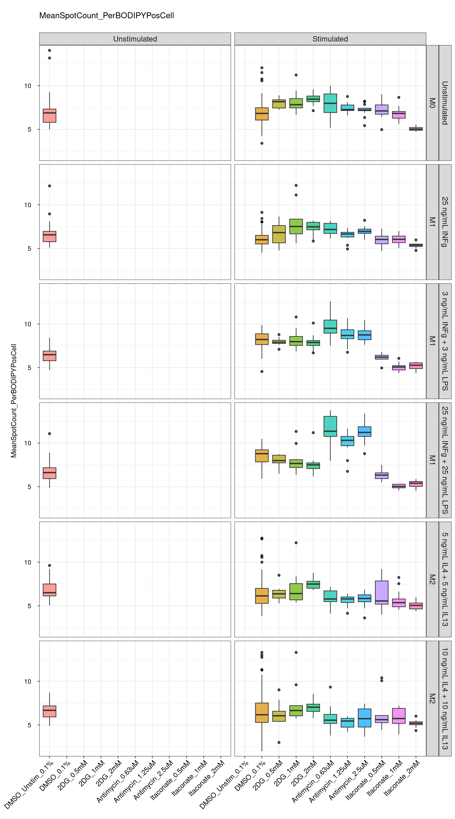

Dot plots

# Print graphs
for (condition in cond_list){

  cat("\n### ", paste0(condition), "{.tabset .tabset-fade .tabset-pills}\n")

  cat("\n#### ", value_list[1], "{.tabset .tabset-fade .tabset-pills}\n")
  print(htmltools::tagList(plotly::ggplotly(
      gen_dotplot(feature_list[7], value_list[1], condition), tooltip = c("Plate", "text"), width = 950, height =350)))
  cat("\n")

  cat("\n##### ", value_list[2], "{.tabset .tabset-fade .tabset-pills}\n")
  print(htmltools::tagList(plotly::ggplotly(
      gen_dotplot(feature_list[7], value_list[2], condition), tooltip = c("Plate", "text"), width = 950, height =350)))
  cat("\n")

  cat("\n###### ", value_list[3], "\n")
  print(htmltools::tagList(plotly::ggplotly(
      gen_dotplot(feature_list[7], value_list[3], condition), tooltip = c("Plate", "text"), width = 950, height =350)))
  cat("\n")
}

Unstimulated

Raw

NormToUnstimDMSO

NormToStimDMSO

25 ng/mL INFg

Raw

NormToUnstimDMSO

NormToStimDMSO

3 ng/mL INFg + 3 ng/mL LPS

Raw

NormToUnstimDMSO

NormToStimDMSO

25 ng/mL INFg + 25 ng/mL LPS

Raw

NormToUnstimDMSO

NormToStimDMSO

5 ng/mL IL4 + 5 ng/mL IL13

Raw

NormToUnstimDMSO

NormToStimDMSO

10 ng/mL IL4 + 10 ng/mL IL13

Raw

NormToUnstimDMSO

NormToStimDMSO

Analysed by Ann Rann Wong

AnnRann.Wong@petermac.org

Victorian Centre for Functional Genomics

sessionInfo()

R version 4.4.2 (2024-10-31)
Platform: x86_64-pc-linux-gnu
Running under: Rocky Linux 9.5 (Blue Onyx)

Matrix products: default
BLAS/LAPACK: FlexiBLAS OPENBLAS-OPENMP;  LAPACK version 3.9.0

locale:
 [1] LC_CTYPE=en_AU.UTF-8       LC_NUMERIC=C              
 [3] LC_TIME=en_AU.UTF-8        LC_COLLATE=en_AU.UTF-8    
 [5] LC_MONETARY=en_AU.UTF-8    LC_MESSAGES=en_AU.UTF-8   
 [7] LC_PAPER=en_AU.UTF-8       LC_NAME=C                 
 [9] LC_ADDRESS=C               LC_TELEPHONE=C            
[11] LC_MEASUREMENT=en_AU.UTF-8 LC_IDENTIFICATION=C       

time zone: Australia/Melbourne
tzcode source: system (glibc)

attached base packages:
[1] stats     graphics  grDevices utils     datasets  methods   base     

other attached packages:
 [1] magick_2.8.5      lubridate_1.9.4   forcats_1.0.0     stringr_1.5.1    
 [5] dplyr_1.1.4       purrr_1.0.4       readr_2.1.5       tidyr_1.3.1      
 [9] tibble_3.2.1      ggplot2_3.5.1     tidyverse_2.0.0   patchwork_1.3.0  
[13] viridis_0.6.5     viridisLite_0.4.2 reshape2_1.4.4    DT_0.33          
[17] readxl_1.4.4      data.table_1.17.0 workflowr_1.7.1  

loaded via a namespace (and not attached):
 [1] gtable_0.3.6      xfun_0.51         bslib_0.9.0       htmlwidgets_1.6.4
 [5] processx_3.8.6    callr_3.7.6       tzdb_0.4.0        vctrs_0.6.5      
 [9] tools_4.4.2       crosstalk_1.2.1   ps_1.9.0          generics_0.1.3   
[13] parallel_4.4.2    pkgconfig_2.0.3   lifecycle_1.0.4   compiler_4.4.2   
[17] farver_2.1.2      git2r_0.35.0      munsell_0.5.1     getPass_0.2-4    
[21] httpuv_1.6.15     htmltools_0.5.8.1 sass_0.4.9        lazyeval_0.2.2   
[25] yaml_2.3.10       plotly_4.10.4     crayon_1.5.3      later_1.4.1      
[29] pillar_1.10.1     jquerylib_0.1.4   whisker_0.4.1     cachem_1.1.0     
[33] mime_0.12         tidyselect_1.2.1  digest_0.6.37     stringi_1.8.4    
[37] labeling_0.4.3    rprojroot_2.0.4   fastmap_1.2.0     grid_4.4.2       
[41] colorspace_2.1-1  cli_3.6.4         magrittr_2.0.3    withr_3.0.2      
[45] scales_1.3.0      promises_1.3.2    bit64_4.6.0-1     timechange_0.3.0 
[49] rmarkdown_2.29    httr_1.4.7        bit_4.5.0.1       gridExtra_2.3    
[53] cellranger_1.1.0  hms_1.1.3         evaluate_1.0.3    knitr_1.49       
[57] rlang_1.1.5       Rcpp_1.0.14       glue_1.8.0        vroom_1.6.5      
[61] rstudioapi_0.17.1 jsonlite_1.9.1    R6_2.6.1          plyr_1.8.9       
[65] fs_1.6.5

MicrobiomeMcConville LabBMDM Screen QC

Aim

Researcher

Readout

Image analysis software

Required R packages

Screen details

Screen dates (yyyy-mm-dd)

Cell lines

Conditions

Screen outline

Controls

Known technical issues

Plate layout

Data cleaning

Data processing

Thresholding

Aggregation

Normalisation

Screen quality - DAPI Count

Heat maps

Total_DAPI_Count

Plate QC Metrics

Total_DAPI_Count

10 ng/mL IL4 + 10 ng/mL IL13

25 ng/mL INFg

25 ng/mL INFg + 25 ng/mL LPS

3 ng/mL INFg + 3 ng/mL LPS

5 ng/mL IL4 + 5 ng/mL IL13

Unstimulated

Box plots

Negative Control

Positive Control

Technical Control

Dot plots

Unstimulated

Raw

NormToUnstimDMSO

NormToStimDMSO

25 ng/mL INFg

Raw

NormToUnstimDMSO

NormToStimDMSO

3 ng/mL INFg + 3 ng/mL LPS

Raw

NormToUnstimDMSO

NormToStimDMSO

25 ng/mL INFg + 25 ng/mL LPS

Raw

NormToUnstimDMSO

NormToStimDMSO

5 ng/mL IL4 + 5 ng/mL IL13

Raw

NormToUnstimDMSO

NormToStimDMSO

10 ng/mL IL4 + 10 ng/mL IL13

Raw

NormToUnstimDMSO

NormToStimDMSO

Screen quality - ARG Positive Perc

Heat maps

Positive_Perc_ARG

Plate QC Metrics

Positive_Perc_ARG

10 ng/mL IL4 + 10 ng/mL IL13

25 ng/mL INFg

25 ng/mL INFg + 25 ng/mL LPS

3 ng/mL INFg + 3 ng/mL LPS

5 ng/mL IL4 + 5 ng/mL IL13

Unstimulated

Box plots

Negative Control

Positive Control

Technical Control

Dot plots

Unstimulated

Raw

NormToUnstimDMSO

NormToStimDMSO

25 ng/mL INFg

Microbiome
McConville Lab
BMDM Screen QC